Detecting seasonal variations in seismic velocities within Los Angeles basin from correlations of ambient seismic noise.

(1)

HAL Id: hal-00704262

https://hal.archives-ouvertes.fr/hal-00704262

Submitted on 5 Jun 2012

HAL is a multi-disciplinary open access archive for the deposit and dissemination of sci-entific research documents, whether they are pub-lished or not. The documents may come from teaching and research institutions in France or abroad, or from public or private research centers.

L’archive ouverte pluridisciplinaire HAL, est destinée au dépôt et à la diffusion de documents scientifiques de niveau recherche, publiés ou non, émanant des établissements d’enseignement et de recherche français ou étrangers, des laboratoires publics ou privés.

Los Angeles basin from correlations of ambient seismic

noise.

Meier Ueli, Florent Brenguier, N. M. Shapiro

To cite this version:

Meier Ueli, Florent Brenguier, N. M. Shapiro. Detecting seasonal variations in seismic velocities within Los Angeles basin from correlations of ambient seismic noise.. Geophysical Journal Interna-tional, Oxford University Press (OUP), 2010, Volume 181 (Issue 2), p. 985-996. �10.1111/j.1365-246X.2010.04550.x�. �hal-00704262�

(2)

Detecting seasonal variations in seismic velocities within Los

Angeles basin from correlations of ambient seismic noise

Ueli Meier

12

, Nikolai M. Shapiro

1

, Florent Brenguier

1

Institut de Physique du Globe de Paris, Equipe de Sismologie 4 Place Jussieu Case 89, 75252 Paris cedex 05, France. 2

Now at: IDSIA, Galleria 2, 6928 Manno-Lugano, Switzerland. Email: meierue@ipgp.jussieu.fr

SUMMARY

We analyze 3 years of continuous seismic records from broadband stations of the Caltech Re-gional Seismic Network (CI) in vicinity of the Los Angeles basin. Using correlations of ambi-ent seismic noise, relative velocity variations in the order of 0.1 % can be measured between all inter-station pairs. It is the first time that such an extensive study between 861 inter-station pairs over such a large area has been carried out. We perform these measurements using the ’stretching’ technique, assuming that one of the two waveforms is merely a stretched version of the other. Obviously this assumption is always violated and the two waveforms are gener-ally decorrelated due to temporal changes in the Earth crust, due to different sources or simply because the cross-correlations are not fully converged. We investigate the stability of these measurements by repeating each measurement over various time-windows of equal length. On average between all inter-station pairs in the Los Angeles basin a seasonal signal in the relative velocity variation is observed, with peaks and troughs during winter and summer time respectively. Generally the observed signal decreases with increasing inter-station distance and relative travel-time perturbations can only be measured up to an inter-station distance of 60 km. Furthermore the travel-time perturbations do not depend on azimuth of station pairs, suggest-ing that they are not related to seasonal variations of the noise sources. Performsuggest-ing a simple

(3)

regionalization by laterally averaging measurements over a subset of stations we found the sedimentary basin showing the most consistent signal and conclude that the observed season-ality might be induced either by changes in the ground-water aquifer or thermo-elastic strain variations that persist down to a depth of 15-22 km.

Key words: Seismic noise, Interferometry, Crustal structure

1 INTRODUCTION

It has become common ground in seismology that the cross-correlation of a random wave field sensed at two different seismic stations yields the Green’s function between the two stations (e.g. Weaver & Lobkis, 2001; Larose et al., 2006; Gou´edard et al., 2008). An immediate consequence of this theorem, is that any seismic instrument can be used as a potential source, resulting in increased lateral resolution compared to conventional active seismic imaging. It has been demonstrated that surface wave Green functions can be extracted by cross-correlation of multiply scattered seismic coda (Campillo & Paul, 2003), as well as by cross-correlation of ambient seismic noise (Shapiro & Campillo, 2004; Sabra et al., 2005a,b; Shapiro et al., 2005). This new data source has been exploited extensively to perform conventional surface wave dispersion measurements on local and regional scale (e.g. Brenguier et al., 2007; Lin et al., 2007; Moschetti et al., 2007; Stehly et al., 2009).

In all this studies the surface waves were retrieved from continuous ambient seismic noise records of a given duration and treated as being stationary. Green’s functions retrieved from am-bient seismic noise records over different time periods are strictly speaking not stationary, and the temporal variations contain useful information. Exploring these temporal variations, it is for example possible to detect instrumental errors (Stehly et al., 2007; Sens-Sch¨onfelder, 2008) or to estimate slight changes in the seismic velocity structure. Temporal variations of the media seis-mic velocity are generally too small to be detected by direct waves. The longer the waves travel through the medium the more sensitive they become to velocity variations. Latter arriving phases, generally attributed to multiply scattered waves, are therefore of great potential to detect rela-tive temporal variations in the subsurface. Estimating relarela-tive changes in the mean shear wave

(4)

velocity from comparison of multiply scattered coda waves dates back to Poupinet et al. (1984), who measured temporal variations of crustal velocities from seismograms recorded from a pair of micro-earthquakes occurring at different dates with nearly identical hypocenter and magnitude. Such events are however very rare, which explains the limited applicability of this technique. Ex-periments with repeated active seismic sources are also a possibility to obtain similar waveforms but are in general rather expensive (e.g. Nishimura et al., 2000; Wegler et al., 2006). In contrast, continuous ambient seismic noise records from permanent or semi-permanent networks are more cost effective and furthermore the position of the receivers and hence the apparent sources does not change with time. Sens-Schönfelder & Wegler (2006) demonstrated that Green’s functions retrieved from ambient seismic noise records contain multiply scattered waves, which can be an-alyzed to monitor small temporal variations of the subsurface. Indeed, this technique has been successfully applied to detect small velocity variations in volcanoes (e.g. Sens-Schönfelder & We-gler, 2006). Similarly, Wegler & Sens-Schönfelder (2007) and Brenguier et al. (2008a) detected a decrease of relative seismic velocities that coincidence with the occurrence of an earthquake and Brenguier et al. (2008b) detected a decrease in relative velocity prior to volcanic eruptions. The same principle has also been successfully applied in laboratory experiments to detect small varia-tions in the medium of interest (e.g. Snieder et al., 2002; Grêt et al., 2006; Leroy & Derode, 2008; Larose & Hall, 2009; Hadziioannou et al., 2009).

In this paper we extend this technique to broadband data from the Caltech Regional Network (CI) and analyze 3 years of continuous seismic records from 42 broadband stations. It is for the first time that such an extensive study, analyzing relative velocity changes from 861 inter-station pairs covering an area of approximately 90 × 190 km, has been carried out. We measured relative traveltime perturbations between all the inter-station pairs in various frequency bands between 0.1 to 2 Hz in the Los Angeles basin. We mainly opted for this frequency band because it in-cludes the micro-seismic peak (Stehly et al., 2006). We perform repeated measurements over var-ious time-windows and computed corresponding uncertainties from the variance of those repeated measurements. In principle these uncertainties should depend on the amount of decorrelation as described by the correlation coefficient, central frequency, bandwidth and length of the time

(5)

win-dow over which the measurements are performed (Hadziioannou et al., 2009; Weaver et al., 2009). Our uncertainty estimates do however not depend on the maximum correlation coefficient and we therefore decided to discard measurements from two waveforms whose maximum correlation co-efficient after stretching is below a certain threshold. In this way we simply discard bad quality measurements from further analysis. Using a simple regionalization scheme, laterally averaging measurements from a subset of stations, we were able to identify the sedimentary basin as having the most consistent signal. These are however still preliminary and qualitative results. In order to further improve on these results and quantitatively map relative velocity changes in the Earth’s crust on regional scale a better understanding of the spatial sensitivities of these measurements is required. A problem that to the best of our knowledge is still an open issue.

2 DATA

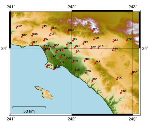
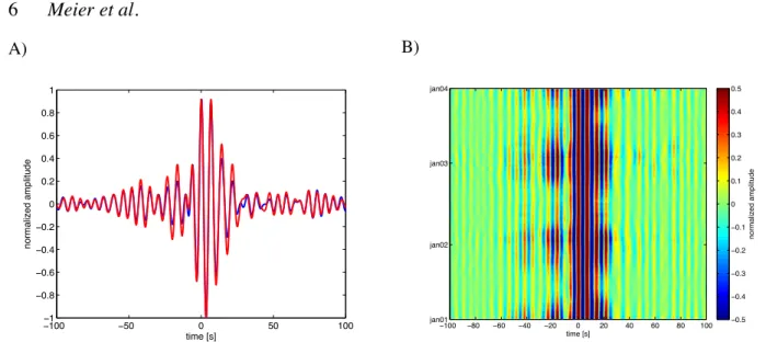
We analyzed 3 years of continuous seismic records from 42 broadband stations of the Caltech Regional Network (CI) in the vicinity of the Los Angeles basin (Fig. 1). Not only are we using many more stations than in previous studies but also cover a much bigger area with a maximum inter-station distance of ≈ 190 km parallel to the coast (DGR-MOP) and ≈ 90 km perpendic-ular to the coast (BFS-RPV). The data were obtained from the Southern California Earthquake Data Center (SCEDC). We only analyzed the vertical component and performed standard data processing: 1) removed the instrument response, 2) down-sampled the data to a sampling rate of 0.05 s, 3) performed spectral whitening in the frequency band of 0.0064-4 Hz, 4) applied one-bit normalization and 5) computed 1-day cross-correlations for all the 861 inter-station pairs and 42 auto-correlations for a time-lag of ±600 s. Stacking the 1 day correlations over the whole 3 year time period results in the reference stack. In order to measure the temporal evolution of relative traveltime perturbations with respect to the reference stack, we computed 60 day-long stacks over the whole 3 year period in a five day moving window. In Figure 2 a 60-day stack together with the reference stack is shown for the station-pair DEC-USC (A), as well as all 60-day stacks over the whole 3-year period for the same station-pair (B). Note that slight changes in coherent phases

(6)

241˚ 241˚ 242˚ 242˚ 243˚ 243˚ 34˚ 34˚ 50 km BCC BFS BRE CAP CHN CLT CPP DEC DGR DJJ DLA FMP HLL LAF LCG LGB LLS LTP MLS MOP MWC OLI PDR PDU PLS RIN RIO RPV RSS RUS SDD SMS SPF SRN STG STS SVD TOV USC _WLT WSS WTT

Figure 1. 42 broadband stations indicated by the red circles of the Caltech Regional Network (CI) consid-ered in this study.

arriving after ±25 s over the 3-year period are already visible. Furthermore seasonal variations in amplitudes of the 60-day stacks are also visible.

3 MEASURING RELATIVE VELOCITY PERTURBATIONS

By measuring relative velocity perturbations (δv/v) from the coda of two similar waveforms it is generally assumed that δv/v is spatially homogeneous. This implies that the relative time shift (δτ /τ ) between the two waveforms is independent of the lapse time (τ ) at which it is measured and δv/v = −δτ /τ = const. (Snieder et al., 2002). In principle it would be sufficient to measure δτ at one particular lapse time τ to estimate δτ /τ . Mainly because the relative velocity perturbations are only approximately homogeneous but also due to uncertainties in measuring δτ a statistical

approach is generally chosen and δτiis measured at various laps times τi.

There are two similar techniques to measure δτi within time windows of length T centered

(7)

A) −100 −50 0 50 100 −1 −0.8 −0.6 −0.4 −0.2 0 0.2 0.4 0.6 0.8 1 time [s] normalized amplitude B) time [s] −100 −80 −60 −40 −20 0 20 40 60 80 100 jan01 jan02 jan03 jan04 normalized amplitude −0.5 −0.4 −0.3 −0.2 −0.1 0 0.1 0.2 0.3 0.4 0.5

Figure 2. A) Sixty-day stacked cross-correlation function starting at 01/05/2001 (blue) together with the 3-year reference stack (red) for station-pair DEC-USC. B) All 60-day stacks over the 3-year period for station-pair DEC-USC. The cross-correlations are filtered between 0.1-0.2 [Hz].

the cross-correlation of the two waveforms in each window of length T centered around τi. δτ /τ

is then approximated as the mean of all δτi/τimeasured over a window of length L, where L > T .

Another technique estimates δτi from the phase of the cross-spectrum of the two waveforms in

each window of length T centered around τi. The time shift δτi is then obtained by fitting a line,

starting at the origin, to the phase of the cross-spectrum φ(f ) = 2πδτif (Poupinet et al., 1984).

With this technique the accuracy of the individual measurements is not limited by the sampling

rate. δτ /τ and hence δv/v is then obtained by a linear regression of the various δτi measurements

over a window of length L, where L > T . Both techniques require to choose an appropriate value for the window length T , which should be long enough to obtain meaningful correlations and cross-spectra but also short enough to ensure that the distortion of the two waveforms is small within these windows. Sens-Sch¨onfelder & Wegler (2006) proposed instead to estimate δτ /τ as the factor by which the time axis on one waveform has to be stretched or compressed to obtain the best correlation with the other waveform over the time-window of length L. An obvious advantage to the above mentioned techniques, is that there is no need to set an appropriate value for T and more importantly, a direct estimate of δτ /τ is obtained. In a recent study Hadziioannou et al. (2009) discussed advantages and drawbacks of both above mentioned techniques.

(8)

3.1 Uniform scaling of the time axis (Stretching)

More formally, let’s assume we have two waveforms, a reference waveform fref_{(t) and a current}

waveform fcur_{(t). A stretched version of f}cur_{(t) is defined as:}

fcur

! (t) = f

cur_{(t(1 + %))} ₍₁₎

where % is the stretching coefficient. When then look for % that maximizes:

C(%) = ! fcur ! (t)fref(t)dt " (! fcur ! (t) 2 dt)(! fref_(t)2 dt) (2)

where integration is over a specific time window t1 <= t <= t2 of length L = t2 −t1 and the

relative time shift of fcur_{with respect to f}ref _{is simply given by: δτ /τ = −%}

max.

If fcur _{is a stretched version of f}ref_{, we will find C}

max = 1 at some %max $= 0. In general

the two waveforms fcur _{and f}ref _{will slightly differ due to temporal variations in the Earth crust,}

due to different sources or because the correlations are not fully converged (i.e. Cmax < 1). Strong

distortion and weak stretching might furthermore indicate a change of structure rather than a global velocity change. In other words, the assumptions on which eq. (2) are based are always going to be

violated, leading to errors in the estimation of %max. It is therefore crucial to investigate the stability

of the measurements as well as trying to come up with uncertainty estimates that serve as a measure of how reliable a particular measurement is. So far it has been shown that increasing the window length L and/or the bandwidth can reduce the effect of differing waveforms (Hadziioannou et al., 2009). It is however still an unresolved issue how slightly differing waveforms are affecting the estimation of the stretching coefficient (Weaver et al., 2009).

Here we take a pragmatic approach in order to investigate the stability of the performed mea-surements and perform repeated meamea-surements in shifted but overlapping time-windows of equal length. If one of the two waveforms is merely a stretched version of the other, all repeated mea-surements should yield identical results. The variance of the repeated meamea-surements can therefore be seen as an error estimate of the δτ /τ measurements. Additionally we also keep track of the maximum value of the correlation coefficient and discard measurements whose best stretching

(9)

co-efficient results in a correlation coco-efficient below a certain threshold. In this way measurements from waveforms that differ too much are simply excluded.

In order to measure relative time-shifts in the coda of a 60-day stack with respect to the ref-erence stack an appropriate time window has to be chosen. We computed cross-correlations for a time-lag of ±600 s. In order to obtain meaningful measurements of δτ /τ this is obviously to long and since we are interested in comparing measurements for different inter-station distances

up to 189 km, an adaptive starting time (t1) of the time window has to be chosen. Since we are not

interested in direct surface waves we set for all inter-station pairs the starting time t1 = di/vmin,

where di is the ith inter-station pair distance and vmin = 1 k/s is the surface wave velocity. In

order to adapt the window length to different frequency ranges the time window length is set to

L = 10Tmax, where Tmaxis the maximum period of the considered bandwidth. When then repeat

the measurement k times in a smaller time window of length L = 5Tmax and increased starting

time tstart = t1+(k −1)T_max, where k = 1, .., 5 (Fig. 3). From the five independent measurements

in smaller time windows we compute error estimates of %maxaround the values estimated from the

measurement performed over the long time window.

In Figure 4 the cross-correlation as a function of the stretching coefficient (eq. 2) is shown for a 60-day stack starting at 01/05/2001 with respect to the 3-year reference stack for station-pair BRE-CHN in the negative (A) and positive (B) time windows, respectively. The dashed lines are

com-puted in overlapping time-windows of length L = 50s with starting times t1 = ±35, ±45, .., ±85s,

and the solid line is computed over a time window of length L = 100s starting at t1 = ±35. A

zoom around the maximum is shown in (C) and (D) with the stretching coefficient that maximizes eq. 2 (solid vertical line), and the uncertainties (dashed line) given by the standard deviation of the repeated measurements over the shorter time windows (dashed curves in A,B). The value of the correlation coefficient gives a measure of how well the two waveforms match after stretching, and we would intuitively guess that the lower the maximum correlation coefficient the lower the qual-ity of the measurements. In section 4 we will demonstrate how only considering measurements with a correlation coefficient bigger than a certain threshold increases the quality of the result.

(10)

−150 −100 −50 0 50 100 150 −1.5 −1 −0.5 0 0.5 1 1.5 time [s] normalized amplitude

Figure 3. Sixty-day stacked cross-correlation function filtered between 0.1-0.2 Hz starting at 01/05/2001 (blue) together with the 3-year reference stack (red) for station-pair BRE-CHN. The time window of length L = 10Tmax (black box) and the time window of length L = 5Tmax (black dashed box) that is shifted towards the right and over which the relative time shifts are measured repeatedly is also shown for positive lapse times.

In this example we evaluated C(%) for stretching coefficients ranging from [−0.1 : 0.1] with

an increment of ∆% = 10−4, the resulting %

max has therefore an accuracy of 10−

4

and 2001 eval-uations of C(%) are required to find the maximum. This is obviously far from being efficient and considering that we ultimately perform 207 measurements for 861 inter-station pairs in positive and negative time windows a more efficient algorithm to maximize C(%) is required. We opted for

a line search algorithm (Nabney, 2002) that allows us to estimate Cmax with an accuracy of 10−

4

requiring much less evaluations of %max. The increased efficiency came however at the price, that

we risk to find only a local maximum. It is therefore crucial to chose appropriate initial bounds on %. If the initial search bound is too broad, there are likely to be various maxima in the correla-tion coefficient funccorrela-tion C(%), if the initial search bound is however too narrow, there might be no maximum at all and our results might be biased. In other words, the initial search bound reflects

(11)

A) −0.1 −0.05 0 0.05 0.1 −1 −0.8 −0.6 −0.4 −0.2 0 0.2 0.4 0.6 0.8 1 stretching coefficient ε CC( ε ) B) −0.1 −0.05 0 0.05 0.1 −1 −0.8 −0.6 −0.4 −0.2 0 0.2 0.4 0.6 0.8 1 stretching coefficient ε CC( ε ) C) −0.01 −0.005 0 0.005 0.01 0.5 0.55 0.6 0.65 0.7 0.75 0.8 0.85 0.9 0.95 1 stretching coefficient ε CC( ε ) D) −0.01 −0.005 0 0.005 0.01 0.5 0.55 0.6 0.65 0.7 0.75 0.8 0.85 0.9 0.95 1 stretching coefficient ε CC( ε )

Figure 4. Correlation coefficient as a function of the stretching coefficient (eq. 2) computed over 100s long (solid) and 50s long (dashed) windows for the two waveforms shown in Fig. 3 for negative (A) and positive (B) lapse times. (c) and (D) show a zoom around the maximum of the cross correlation function of the 100_{s long window (solid) together with the maximum (vertical line) and the corresponding uncertainties} (dashed) estimated from the 5 repeated measurements over 50s long windows. Note the different horizontal scale in (C) and (D).

the maximum traveltime perturbations between a 60-day and the reference stack we are expecting a priori. After evaluating and plotting C(%) for various inter-station pairs in the different frequency bands considered, we set the initial search range to −0.01 <= % <= 0.01 for the frequency ranges 0.1-0.2, 0.1-1 and 0.1-2 Hz and to −0.005 <= % <= 0.005 for the frequency range 0.5-2 Hz respectively.

(12)

4 RESULTS

We measured δτ /τ from all the 207, 60-day stacks with respect to the reference stack for all

861 inter-station pairs in a particular time window of length L starting at ±t1. Additionally we

computed the corresponding standard deviations as the variance of the repeated measurements. In total we performed 6 × 178227 measurements in positive and negative time windows. Perform-ing that many measurements requires an automated quality control of the 60-day stacked cross-correlations. There are various problems that might arise, limited data availability during some days, missing information about the instrument response on other days, or unknown instrumental time-shifts for some stations, just to name a few. If one of the above mentioned problems arose during a particular time-period, the resulting 60-day stacks are likely to be corrupted. In order to detect those spurious correlations we first check if the two waveforms are correctly aligned and only perform measurements if the maximum of the cross-correlation in the considered time win-dow occurs at time lags smaller than ±5 times the sampling rate. In this way we reject spurious waveforms that for one reason or another are not suitable to perform the measurements and ulti-mately would degrade the results. For illustrative purposes we start presenting our results with a comparison from one particular inter-station pair in various frequency bands.

4.1 Comparison of δτ /τ for BRE-CHN, in four different frequency ranges: 0.1-0.2, 0.1-1

0.1-2 and 0.5-2 Hz

We measured δτ /τ from 207, 60-day stacks with respect to the reference stack for the inter-station pair BRE-CHN and compare the obtained results from cross-correlations filtered between 0.1-0.2, 0.1-1, 0.1-2 and 0.5-2 Hz. In Figure 5, the outcome of this comparison is summarized: δτ /τ mea-surements are shown together with the corresponding standard deviations in the positive (blue) and

negative (red) time window (left column); the corresponding Cmax values are shown for positive

(blue) and negative (red) time windows (middle column); and all the 207, 60-day stacks in the considered time windows are shown (right column). From top to bottom the corresponding cross-correlations where filtered between 0.1-0.2 (A-C), 0.1-1 (D-F), 0.1-2 (G-I) and 0.5-2 Hz (J-L).

(13)

values are an indication that the 60-day stack is not merely a stretched/compressed version of the reference stack, and that the two waveforms are highly decorrelated. In this case the correspond-ing estimates of δτ /τ are obviously less precise and ultimately meancorrespond-ingless. This observation is

most evident in the frequency range between 0.5-2 Hz, where the Cmaxvalues in the positive time

window (K, blue) are very low. Looking at the waveforms (L, right panel) this is not surprising be-cause there are no coherent phases in this frequency range. Since the inter-station pair BRE-CHN is perpendicular to the coast, the positive time window corresponds to waves traveling towards the ocean, a direction which is known to have very weak noise sources. The same observation can be made for the other three frequency ranges, but to a lesser extent. Furthermore it is worth noting that δτ /τ in the positive and negative time windows show a seasonal variation with peaks and troughs during winter and summer time respectively. The amplitude of this variations is in the order of ±0.5% in the frequency range between 0.1-0.2 Hz (A) and in the order of ±0.2% in the frequency ranges 0.1-1 Hz (D) and 0.5-2 Hz (G) respectively.

4.2 Laterally averaged distribution of δτ /τ for all 861 inter-station pairs

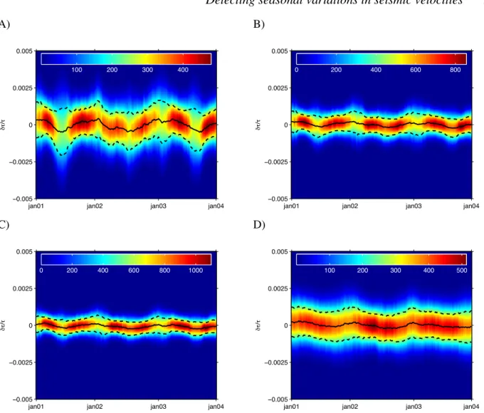
In a next step we computed averages and standard deviations of δτ /τ from all the 861 inter-station pairs. Instead of only plotting mean and standard deviations we decided to plot the whole Gaus-sian distribution for each time step over the whole 3-year period (Fig. 6), merely for illustrative purposes. Each vertical line on these plots corresponds to a Gaussian probability density function pdf (i.e. integrates to unity) with mean and standard deviation computed as described in section (3.1). This figure can be seen as a summary of all the performed measurements. The mean (black line) shows a clear seasonal variation. Note however that standard deviations are rather big espe-cially for the frequency range between 0.1-0.2 Hz (Fig. 6A). This might be due to the fact that we averaged measurements over various inter-station pair distances, ranging from 6-190 km, various azimuths of station pairs and considered all paths that correspond to varying geological regimes. The more likely reason for this high standard deviations is however the small bandwidth that makes the measurements less stable to distortions of the waveforms (Hadziioannou et al., 2009). And indeed as can be seen for the other frequency bands the broader the bandwidth the more

(14)

A)

jan01 jan02 jan03 jan04

−0.01 −0.005 0 0.005 0.01 δτ /τ B)

0.2 0.3 0.4 0.5 0.6 0.7 0.8 0.9 1 max. CC C) −120 −100 −80 −60 −40 jan01 jan02 jan03 jan04 time [s] 40 60 80 100 120 D)

−0.005 −0.0025 0 0.0025 0.005 δτ /τ E)

0.55 0.6 0.65 0.7 0.75 0.8 0.85 0.9 0.95 1 max. CC F) −120 −100 −80 −60 −40 jan01 jan02 jan03 jan04 time [s] 40 60 80 100 120 G)

−0.005 −0.0025 0 0.0025 0.005 δτ /τ H)

0.2 0.3 0.4 0.5 0.6 0.7 0.8 0.9 1 max. CC I) −120 −100 −80 −60 −40 jan01 jan02 jan03 jan04 time [s] 40 60 80 100 120 J)

−0.01 −0.005 0 0.005 0.01 δτ /τ K)

0.1 0.2 0.3 0.4 0.5 0.6 0.7 0.8 0.9 1 max. CC L) −55 −50 −45 −40 −35 jan01 jan02 jan03 jan04 time [s] 35 40 45 50 55

Figure 5. A) Relative time shift measurements and corresponding standard deviations of all 207, 60-day stacks with respect to the reference stack, measured in the positive (blue) and negative (red) time window (L = 100 s) for the inter-station pair BRE-CHN in the frequency range between 0.1-0.2 Hz . B) Values of the maximum correlation coefficient Cmaxin the positive (blue) and negative (red) time window. C) All the 207, 60-day stacks filtered between 0.1-0.2 Hz, only the time windows over which the measurements were performed are shown. D-F) Similar plots as A-C) only that the cross-correlations are filtered between 0.1-1 Hz. G-I) Similar plots as A-C) only that the cross-correlations are filtered between 0.1-2 Hz. J-L) Similar plots as A-C) only that the cross-correlations are filtered between 0.5-2 Hz, note the shorter window length of L = 50 s. Vertical axes are changing in left and middle columns.

(15)

stable the measurements are. Another problem is that we considered all the measurements, some of this measurements are potentially from waveforms that differ too much even after stretching. Consequently the maximum correlation coefficient of those measurements is low and indeed if all

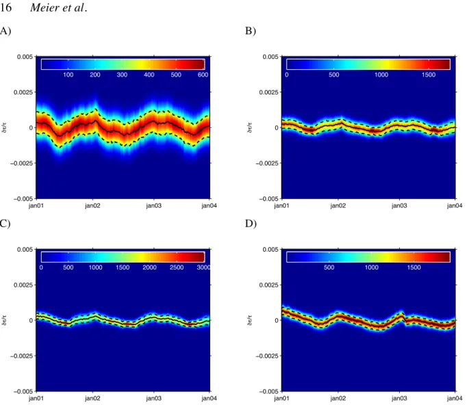
measurements with Cmax < 0.9 are excluded the resulting standard deviation of the distribution

of δτ /τ is much smaller (Fig. 7).We conclude that seasonal variations of δτ /τ measurements with peaks and troughs during winter and summer time respectively are a robust feature in the studied area and that in order to obtain more robust results the bandwidth can be increased. Furthermore

it is crucial to exclude measurements from waveforms that differ too much as described by Cmax.

In what follows we will focus further discussion of the results on the seasonal variations and will only consider measurements performed over the frequency range 0.1-2 Hz.

4.3 Relative time shifts as a function of inter-station pair distance

In order to further investigate the origin of the observed signal we decided to investigate the depen-dence of δτ /τ with respect to inter-station pair distance. In Figure 8, the distribution of the average is plotted for 6 different inter-station pair distances, 0-20 (top,left), 20-40 (top,right), 40-60 (mid-dle,left), 60-80 (middle,right), 80-100 (bottom,left) and for inter-station pair distances > 100 km (bottom,right). Note that between 40-60 km the signal becomes weaker and finally disappears completely. This suggests that in the frequency range considered (0.1-2 Hz), seasonal variations in δτ /τ can only be observed for inter-station pair distances up to 40-60 km. A possible explanation for this observation might be, that no coherent phases are present in the considered time-windows for long inter-station pair distances due to attenuation. Looking at the histogram of the maximum correlation coefficient as a function of inter-station pair distance (Fig. 9) it is nicely visible that the bigger the inter-station-pair distance the smaller the corresponding maximum correlation co-efficient of the stretched waveforms become. For long inter-station pair distances stacking only 60-days of ambient seismic noise records is probably not long enough. Consequently the 60-days stack didn’t fully converge and differ too much with respect to the three year-long reference stack. This suggests that if measurements from varying inter-station pair distances were to be combined, an adaptive way on how to choose the stacking duration would be required.

(16)

A)

δτ

/τ

−0.005 −0.0025 0 0.0025 0.005 100 200 300 400 B) δτ /τ

−0.005 −0.0025 0 0.0025 0.005 0 200 400 600 800 C) δτ /τ

−0.005 −0.0025 0 0.0025 0.005 0 200 400 600 800 1000 D) δτ /τ

−0.005 −0.0025 0 0.0025 0.005 100 200 300 400 500

Figure 6. Gaussian pdfs of δτ /τ with superimposed mean (black) ± one standard deviation (dashed) for all 861 inter-station pairs over a 3 year period in various frequency bands, 0.1-0.2 (A), 0.1-1 (B),0.1-2 (C) and 0.5-2 Hz (D).

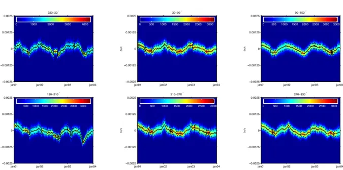
4.4 Relative time shifts as a function of azimuth

It is well documented that the origin of seismic noise sources shows a clear seasonal variation (e.g. Stehly et al., 2006; Yang et al., 2007). In order to investigate if our observations are related to seasonal variations of the seismic sources or rather related to seasonal changes in the subsurface we investigated the dependence of δτ /τ on azimuth of station pairs. If we were measuring some process related to seasonal variations of the seismic sources, that show a clear dependence on azimuth, we would expect to see the same dependence in our δτ /τ measurements. In Figure 10, δτ /τ is plotted as a function of azimuth in the frequency range 0.1-2 Hz. Interestingly there seems to be no particular dependence on azimuth, for all six azimuth bins the same seasonal variations

(17)

A)

δτ

/τ

−0.005 −0.0025 0 0.0025 0.005 100 200 300 400 500 600 B) δτ /τ

−0.005 −0.0025 0 0.0025 0.005 0 500 1000 1500 C) δτ /τ

−0.005 −0.0025 0 0.0025 0.005 0 500 1000 1500 2000 2500 3000 D) δτ /τ

−0.005 −0.0025 0 0.0025 0.005 500 1000 1500

Figure 7. Gaussian pdfs of δτ /τ from high quality measurements(i.e. Cmax > 0.9) with superimposed mean (black) ± one standard deviation (dashed) for all 861 inter-station pairs over a 3 year period in various frequency bands, 0.1-0.2 (A), 0.1-1 (B), 0.1-2 (C) and 0.5-2 Hz (D).

are observed. This suggests that our observations are indeed related to variations in the Earth crust and not due to seasonal variations in the noise sources.

4.5 Crude regionalization

We perform a crude regionalization by simply averaging measurements from inter-station pairs that belong to three different regions. We decided to form three different clusters as indicated in Figure 11A. Cluster 1 (red) consists of stations in the north-western part of the study area mainly on hard-rock sites (Fig. 11B). Cluster 2 (blue) consists of stations in the north-eastern part of the study area, again mainly located on hard-rock sites (Fig. 11C). Whereas cluster 3 (green) consists of stations that are in the central part of the study area and are located within the sedimentary

(18)

dist. 0−20 km

δτ

/τ

−0.0025 −0.00125 0 0.00125 0.0025 200 400 600 800 1000 dist. 20−40 km δτ /τ

−0.0025 −0.00125 0 0.00125 0.0025 200 400 600 800 1000 dist. 40−60 km δτ /τ

−0.0025 −0.00125 0 0.00125 0.0025 200 400 600 800 1000 dist. 60−80 km δτ /τ

−0.0025 −0.00125 0 0.00125 0.0025 200 400 600 800 1000 dist. 80−100 km δτ /τ

−0.0025 −0.00125 0 0.00125 0.0025 200 400 600 800 1000 1200 dist. >100 km δτ /τ

−0.0025 −0.00125 0 0.00125 0.0025 200 400 600 800 1000 1200

Figure 8. Gaussian pdfs of δτ /τ with superimposed mean (black) ± one standard deviation (dashed) for all 861 inter-station pairs as a function of inter-station pair distance in the frequency range 0.1-2 Hz.

0 0.5 1 dist. 0−20 km 0 0.5 1 dist. 20−40 km 0 0.5 1 dist. 40−60 km 0 0.5 1 dist. 60−80 km 0 0.5 1 dist. 80−100 km max. CC 0 0.5 1 dist. 100−120 km max. CC

Figure 9. Histograms of the maximum correlation coefficients for all 861 inter-station pairs as a function of inter-station pair distance.

(19)

δτ

/τ

330−30 °

−0.0025 −0.00125 0 0.00125 0.0025 0 1000 2000 3000 4000 δτ /τ 30−90 °

−0.0025 −0.00125 0 0.00125 0.0025 0 500 1000 1500 2000 2500 3000 δτ /τ 90−150 °

−0.0025 −0.00125 0 0.00125 0.0025 0 500 1000 1500 2000 2500 3000 3500 δτ /τ 150−210 °

−0.0025 −0.00125 0 0.00125 0.0025 500 10001500 2000 2500 30003500 δτ /τ 210−270 °

−0.0025 −0.00125 0 0.00125 0.0025 0 500 1000 1500 2000 2500 3000 δτ /τ 270−330 °

−0.0025 −0.00125 0 0.00125 0.0025 0 500 1000 1500 2000 2500 3000

Figure 10. Gaussian pdfs of δτ /τ with superimposed mean (black) ± one standard deviation (dashed) for all 861 inter-station pairs as a function of azimuth for Cmax> 0.9 in the frequency range 0.1-2 Hz.

basin (Fig. 11D). All three clusters consist of roughly the same amount of stations and also cover a similar area. The average distributions of δτ /τ of cluster 1, cluster 2 and cluster 3 are plotted in Figure 11B, C and D respectively. Clearly the average over stations within the sedimentary basin shows the most consistent variation with a clear seasonality in δτ /τ . The average over stations within cluster 2 shows also a seasonal variation, but the variance is much higher and there also seem to exist additional variation over shorter time ranges. In order to further investigate if those short-term variations are simply due to instabilities in the measurements or are indeed related to processes in the upper crust a more detailed investigation would be required.

5 INTERPRETATION

As far as the interpretation of observed relative velocity changes are concerned, it is of great interest not only to monitor these changes, but also to provide an interpretation of what processes might have caused these changes. In labor experiments, under controlled conditions, it has been demonstrated that either changes in stress, temperature or water saturation result in slight velocity changes that can be detected in the coda (e.g. Weaver & Lobkis, 2000; Grˆet et al., 2006; Larose & Hall, 2009). Identifying the processes that might have caused the observed velocity changes in the Earth’s crust poses a more difficult problem. Recent studies presented interpretations of

(20)

A) 241˚ 241˚ 242˚ 242˚ 243˚ 243˚ 34˚ 34˚ DEC DJJ HLL MOP RIN SPF TOV WSS BFS CHN CLT CPP MLS MWC OLI PDU RIO RSS RUS SVD WLT BRE DLA FMP LAF LCG LGB LLS LTP PDR RPV SMS STS USC WTT BRE DLA FMP LAF LCG LGB LLS LTP PDR RPV SMS STS USC WTT B) δτ /τ

−0.0025 −0.00125 0 0.00125 0.0025 0 1000 2000 3000 4000 5000 C) δτ /τ

−0.0025 −0.00125 0 0.00125 0.0025 0 500 1000 1500 2000 2500 D) δτ /τ

−0.0025 −0.00125 0 0.00125 0.0025 0 500 1000 1500 2000 2500 3000

Figure 11. A) Stations that form the three clusters whose average relative time shifts are shown in B) red stations, C) blue stations and D) green stations. Again in B,C,D) Gaussian pdfs of δτ /τ are shown with superimposed mean (solid) ± one standard deviation (dashed).

relative velocity changes observed at volcanoes and across the San Andreas fault (e.g. Brenguier et al., 2008b,a). These studies covered a rather small area and more importantly the candidate processes that might have caused the measured relative velocity changes were known beforehand (i.e. volcanic eruptions, earthquakes) and the seasonal variations were consider as background noise. Sens-Sch¨onfelder & Wegler (2006) on the other hand observed similar seasonal variations and proposed a depth dependent hydrological model that described the seasonality in the observed relative velocity changes solely based on precipitation. This model however was based on the analysis from a single station-pair.

In the following we discuss three different candidate processes that might have caused the observed seasonal variations within the velocity field of the Los Angeles: 1) changes in water

(21)

content, 2) changes in temperature and 3) changes in stress/strain field. Seasonality of climatolog-ical variables, such as temperature, precipitation and oceanic wave height are potentially causing seasonal changes in the mechanical properties of the Earth’s crust. Seasonal variations have also been observed using SAR interferometry and GPS measurements (Bawden et al., 2001; Watson et al., 2002; Argus et al., 2005). In these studies, observed seasonal vertical displacements have been attributed to vertical motion induced by annual variations of the groundwater table (Baw-den et al., 2001). This hypothesis has been confirmed by Watson et al. (2002) who additionally analyzed GPS data and found that the Los Angeles basin becomes most inflated at the beginning of the year after the rainy season when the aquifer should be at a maximum. This inflation may partially explain reduction of seismic velocities that we observe. Moreover, the observed signal is stronger within the sedimentary basin which is also consistent with seasonal changes in hydro-logical parameters. At the same time, surface waves in the frequency range considered 0.1-2 Hz are sensitive down to a depth of 10 km, which may be significantly deeper than layers affected by variations of the aquifer. Therefore, we also consider other seasonal processes such as changes in surface temperature that might affect seismic velocities in the upper crust. It has been demon-strated by Ben-Zion & Leary (1986) and more recently by Prawirodirdjo et al. (2006) that, while changes in surface temperature affect directly only very superficial parts of the crust, they induce thermo-elastic strain variations that persist down to a depth in the order of the surface temperature wavelength. This wavelength of the temperature field has been estimated to range from 15−22 km (Prawirodirdjo et al., 2006) in three different regions within our study area. According to Ben-Zion & Leary (1986) the amplitude of the thermo-elastic strain is over ten times larger than the effect of ≈ 15m changes of water level in a reservoir. It seems more likely that the strongest variations are caused by induced thermo-elastic induced strain variations within the Earth’s upper crust and that the seasonal variations of hydrological parameters simply further enhance these changes.

6 DISCUSSION

We computed broadband cross-correlations from 861 inter-station pairs in the Los Angeles basin and are able to monitor relative travel-time perturbations over a period of three years. It is to

(22)

our knowledge for the first time that these measurements have been performed for that many inter-station pairs covering such a big area. On average we find a clear seasonality in the relative velocity changes that might persist down to a depth of 10-20 km. Variations between different inter-station pairs have however high variance and in order to obtain stable results we had to average over close by inter-station pairs. The results are therefore still rather qualitative and make a detailed interpretation difficult. A major problem we encountered is the trade-off between temporal and lateral resolution. For bigger inter-station pair distances it seems that longer ambient seismic noise records have to be stacked in order to obtain meaningful measurements. An adaptive way to choose the duration over which the reference stack is built as a function of inter-station pair distance might resolve some issues regarding the stability of the measurements. This would however also introduce different time-resolutions for different measurements complicating the interpretation even further.

We demonstrated how high quality measurements of relative velocity changes on a regional scale, covering an area of approximately 90× 150km, from 861 inter-station pairs can be obtained. We were however only able to give an average interpretation of these measurements, averaged over three different regions. In order to provide more localized estimates of the changes in the Earth crust a better understanding of the spatial sensitivities of δτ/ τ measurements - ideally as a function of frequency - is required, as well as a physical model that relates travel-time perturbations to changes in material properties. This would allow us to perform a meaningful regionalization of our measurements, providing interesting insights into the dynamics of the mechanical properties of the Earth’s upper crust.

ACKNOWLEDGMENT

We thank E. Larose, P. Roux, M. Campillo and R.L. Weaver for helpful discussions, R.L. Weaver for communicating his results on the precision of noise-correlation interferometry and Y. Ben-Zion for discussions regarding the thermo-elastic strain variations. All the data were provided by the Southern California Earthquake Data Center (SCEDC). This work was supported by an ANR contract ANR-06-CEXC-005 (COHERSIS) and an EU contract WHISPER.

(23)

References

Argus, D. F., Heflin, M. B., Peltzer, G., Cramp´e, F., & Webb, F. H., 2005. Interseismic

strain accumulation and anthropogenic motion in metropolitan Los Angeles, J. Geophys. Res., 110(B04401), doi:10.1029/2003JB002934.

Bawden, G. W., Thatcher, W., Stein, R. S., Hudnut, K. W., & Peltzer, G., 2001. Tectonic contrac-tion across Los Angeles after removal of groundwater pumping effects, Nature, 412, 812–815. Ben-Zion, Y. & Leary, P., 1986. Thermoelastic strain in a half-space covered by unconsolidated

material, Bull. Seismol. Soc. Am., 76, 1447–1460.

Brenguier, F., Shapiro, N. M., Campillo, M., Nercessian, A., & Ferrazzini, V., 2007. 3-D sur-face wave tomography of the Piton de la Fournaise volcano using seismic noise correlations,

Geophys. Res. Lett., 34, L02305, doi:10.1029/2006GL028586.

Brenguier, F., Campillo, M., Hadziioannou, C., Shapiro, N. M., Campillo, M., Nadeau, R., & Larose, E., 2008a. Postseismic Relaxation Along the San Andreas Fault at Parkfiel from Conti-nous Seismological Observations, Science, 321(5895), 1478–1481.

Brenguier, F., Shapiro, N. M., Campillo, M., Ferrazzini, V., Duputel, Z., Coutant, O., & Nerces-sian, A., 2008b. Towards forecasting volcanic eruptions using seismic noise, Nature Geosience, 126-130, L02305, doi:10.1029/2006GL028586.

Campillo, M. & Paul, A., 2003. Long-Range Correlations in the Diffuse Seismic Coda, Science, 299, 547–549.

Gouédard, P., Stehly, L., Brenguier, F., Campillo, M., de Verdière, Y. C., Larose, E., Margerin, L., Roux, P., Sánchez-Sesma, F. J., Shapiro, N. M., & Weaver, R. L., 2008. Cross-correlation of random fields: mathematical approach and applications, Geophysical Prospecting, 56, 375–393 doi:10.1111/j.1365–2478.2007.00684.x.

Grˆet, A., Snieder, R., & Scales, J., 2006. Time-lapse monitoring of rock properties with wave interferometry, J. Geophys. Res., 111(B03305), doi:10.1029/2004JB003354.

Hadziioannou, C., Larose, E., Coutant, O., Roux, P., & Campillo, M., 2009. Stability of Monitor-ing Weak Changes in Multiply ScatterMonitor-ing Media with Ambient Noise Correlation: Laborartory Experiments, J. Acoust. Soc. Am., 125, in press.

(24)

Larose, E. & Hall, S., 2009. Monitoring stress related velocity variation in concrete with a 2.10−5

relative resolution using diffuse ultrasound, J. Acoust. Soc. Am., 125, 1853–1857.

Larose, E., Margerin, L., Derode, A., van Tiggelen, B., Campillo, M., Shapiro, N. M., Paul, A., Stehly, L., & Tanter, M., 2006. Correlation of random wavefields: An interdisciplinary review,

Geophysics, 71(4), SI11–SI21.

Leroy, V. & Derode, A., 2008. Temperature-dependent diffusing acoustic wave spectroscopy with resonant scatterers, Phys. Rev. E, 77, doi:10.1103/PhysRevE.77.036602.

Lin, F.-C., Ritzwoller, M. H., Townend, J., Bannister, S., & Savage, M. K., 2007. Ambient noise rayleigh wave tomography of new zealand, Geophys. J. Int., 170, 649–666.

Moschetti, M. P., Ritzwoller, M. H., & Shapiro, N. M., 2007. Surface wave tomography of the western Unite States from ambient seismic noise: Rayleigh wave group velocity maps,

Geochem. Geophys. Geosyst., 8(8), A08010, doi:10.1029/2007GC001655.

Nabney, I. T., 2002. Netlab: Algorithms for Pattern Recognition, Advances in Pattern Recogni-tion, Springer Verlag, London, UK.

Nishimura, T., Uchida, N., Sato, H., Ohtake, M., Tanake, S., & Hamaguchi, H., 2000. Temporal changes of the crustal structure associated with the M6.1 earthquake on September 3, 1998 and the volcanic activity of mount Iwate, Japan, Geophys. Res. Lett., 27(2), 269–272.

Poupinet, G., Ellsworth, W. L., & Frechet, J., 1984. Monitoring Velocity Variations in the Crust Using Earthquake Doublets: An Application to the Calaveras Fault, California, J. Geophys. Res., 89(B7), 5719–5731.

Prawirodirdjo, L., Ben-Zion, Y., & Bock, Y., 2006. Observation and modeling of thermoelastic strain in Southern California Integrated GPS Network daily position time series, J. Geophys.

Res., 111(B02408), doi:10.1029/2005JB003716.

Sabra, K., Gerstoft, P., Roux, P., Kuperman, W., & Fehler, M., 2005a. Extracting time-domain green’s function estimates from ambient seismic noise, Geophys. Res. Lett., 32(L03310), doi:10.1029/2004GL021862.

Sabra, K., Gerstoft, P., Roux, P., Kuperman, W., & Fehler, M., 2005b. Surface wave

(25)

doi:10.1029/2005GL023155.

Sens-Sch¨onfelder, C., 2008. Synchronizing seismic networks with ambient seismic noise,

Geo-phys. J. Int., 174, 966–970.

Sens-Sch¨onfelder, C. & Wegler, U., 2006. Passive image interferometry and seasonal varia-tions of seismic velocities at Merapi Volcano, Indonesia, Geophys. Res. Lett., 33, L21302, doi:10.1029/2006GL027797.

Shapiro, N. M. & Campillo, M., 2004. Emergence of broadband Rayleigh waves from correla-tions of the ambient seismic noise, Geophys. Res. Lett., 31, doiL10.1029/2004GL019491. Shapiro, N. M., Campillo, M., Stehly, L., & Ritzwoller, M. H., 2005. High-Resolution

Surface-Wave Tomography from Ambient Seismic Noise, Science, 307, 1615–1617.

Snieder, R., Grˆet, A., Douma, H., & Scales, J., 2002. Coda Wave Interferometry for Estimating Nonlinear Behaviour in Seismic Velocity, Science, 295, 2253–2255.

Stehly, L., Campillo, M., & Shapiro, N. M., 2006. A study of the seismic noise from its long-range correlation properties, J. Geophys. Res., 111(B10306), doi:10.1029/2005JB004237. Stehly, L., Campillo, M., & Shapiro, N. M., 2007. Traveltime measurements from noise

correla-tion: stability and detection of instrumental time-shifts, Geophys. J. Int., 171, 223–230.

Stehly, L., Fry, B., Campillo, M., Shapiro, N. M., Guilbert, J., Boschi, L., & Giardini, D., 2009. Tomography of the alpine region from observations of seismic ambient noise, Geophys. J. Int., 178, 338–350.

Watson, K. M., Bock, Y., & Sandwell, D. T., 2002. Satellite interferometric observations of displacements associated with seasonal groundwater in the Los Angeles basin, J. Geophys. Res., 107(B4, 2074), doi:10.1029/2001JB000470.

Weaver, R. L. & Lobkis, O., 2000. Temperature dependence of diffuse field phase, Ultrasonics, 38, 491–494.

Weaver, R. L. & Lobkis, O., 2001. On the emergence of the Green’s function in the correlations of a diffuse field, J. Acoust. Soc. Am., 110, 3011–3017.

Weaver, R. L., Hadziioannou, C., Larose, E., & Campillo, M., 2009. On the precision of noise-correlation interferometry, in preparation.

(26)

Wegler, U. & Sens-Sch¨onfelder, C., 2007. Fault zone monitoring with passive image interferom-etry, Geophys. J. Int., 168, 1029–1033.

Wegler, U., L¨uhr, B.-G., Snieder, R., & Ratdomopurbo, A., 2006. Increase of shear wave velocity before the 1998 eruption of Merapi volcano (Indonesia), Geophys. Res. Lett., 33, L09303,doi:10.1029/2006GL025928.

Yang, Y., Ritzwoller, M. H., Levshin, A. L., & Shapiro, N. M., 2007. Ambient noise Rayleigh wave tomography across Europe, Geophys. J. Int., 168, 259–274.