Latitudinal distribution of solar wind as deduced from Lyman alpha measurements: An improved method

HAL Id: insu-02889807

https://hal-insu.archives-ouvertes.fr/insu-02889807

Submitted on 3 Feb 2021

HAL is a multi-disciplinary open access

archive for the deposit and dissemination of

sci-entific research documents, whether they are

pub-lished or not. The documents may come from

teaching and research institutions in France or

abroad, or from public or private research centers.

L’archive ouverte pluridisciplinaire HAL, est

destinée au dépôt et à la diffusion de documents

scientifiques de niveau recherche, publiés ou non,

émanant des établissements d’enseignement et de

recherche français ou étrangers, des laboratoires

publics ou privés.

Latitudinal distribution of solar wind as deduced from

Lyman alpha measurements: An improved method

T. Summanen, Rosine Lallement, Jean-Loup Bertaux, E. Kyrölä

To cite this version:

T. Summanen, Rosine Lallement, Jean-Loup Bertaux, E. Kyrölä. Latitudinal distribution of solar

wind as deduced from Lyman alpha measurements: An improved method. Journal of

Geophys-ical Research Space Physics, American GeophysGeophys-ical Union/Wiley, 1993, 98 (A8), pp.13215-13224.

�10.1029/93JA00144�. �insu-02889807�

JOURNAL OF GEOPHYSICAL RESEARCH, VOL. 98, NO. A8, PAGES 13,215-13,224, AUGUST 1, 1993

Latitudinal Distribution of Solar Wind as Deduced From Lyman Alpha

Measurements'

An Improved Method

T. SUMMANEN

Finnish Meteorological Institute, Helsinki, Finland

R. LALLEMENT AND J. L. BERTAUX

Service d'Aeronomie du Centre National de la Recherche Scientifique, Verridres-le-Buisson, France

E. KYROL)!,

Finnish Meteorological Institute, Helsinki, Finland

In this work we examine the possibility of deducing the latitudinal distribution of the solar ionization rate using Prognoz 6 Lyman alpha data in a more general and flexible way than previously examined. Using so- called hot model for the hydrogen distribution and the optically thin model for the resonance scattering, theoretical Lyman alpha intensity for the interstellar hydrogen is calculated and compared with the intensity data measured by Prognoz 6. Varying the latitudinal dependence of the ionization rate, the distributions, which produce the best fit with the data, are analyzed for four ddferent measuring sessions. As a result, we get four ionization rate distributions that have two common features. The ionization rate is enhanced near the solar equator, and large broad plateaus exist around heliographic latitudes +30 ø to +70 ø. The latitudinal distribution of the average ionization rate about the solar minimum deviates clearly from the spherically symmetric and sinusoidally (harmonically) with the latitude-varying models used so far. The growth of the solar wind mass flux from the solar polar areas toward the equator corresponds to the earlier results concluded from Lyman alpha measurements. The method used in this work allows a higher latitudinal resolution of the ionization rates. However, there are several uncertainties both in the simulations and in the measurements. The exclusion of time-dependent effects as well as multiple scattering requires that the results be considered only suggestive.

1. INTRODUCTION

Studies of coronal holes in the 1970s have led to the

development of a model for the spatial structure of the solar wind. The solar polar regions develop into large coronal holes during the declining phase of the solar cycle, and the holes begin to expand toward the equator. The polar holes attain their greatest size at the minimum phase. At the maximum phase they disappear. The temporal variations of coronal holes suggested latitudinal changes in the solar wind proton flux, which is the main ionizing effect of the interplanetary hydrogen.

At the same time, the interplanetary scintillation (IPS) observations showed that the average solar wind speed increases from the equator toward the polar regions [Coles and Rickett, 1976]. It was discovered that the major sources of the

low-speed flow are distributed along the neutral lines through

the whole solar cycle. During low solar activity the neutral line

lies almost parallel to the solar equator. The high-speed flows

seem to originate then from the polar coronal holes. An extensive review concerning solar wind speed structure

observed

using

the IPS method

from 1973 to 1987 has been

published recently by Kojima and Kakinuma [1990].

Until 1975, spherically-symmetric solar radiation fields for both corpuscular and electromagnetic radiation were assumed while modeling of the neutral hydrogen distribution. Then Joselyn and Holzer [1975] studied theoretically the effect of

Copyright 1993 by the American Geophysical Union.

Paper number 93JA00144. 0148-0227/93/93JA-00144505.00

anisotropic solar wind on the Lyman o• sky background. They assumed that the solar wind proton flux would increase near the polar regions and concluded that latitudinal variations would cause a significant change in the Lyman • intensity. Kumar and Broadfoot [1978, 1979] studied the solar wind's latitudinal structure by comparing the Mariner 10 Lyman • observations and the theoretically calculated intensities. According to their

studies the harmonic ionization rate clearly better fits the data than the spherically symmetric model. The same latitudinal structure has been used also by many other authors [Wittet al.,

1979, 1981; lsenberg and Levy, 1978; Lallement et al.,

1985b].

The main reason to use the harmonic model is that it allows

an analytical evaluation of the hydrogen atom loss rate.

However, the latitudinal variations of the ionization rate seem

to be so fast that the slowly varying harmonic model cannot model them. The independent studies of the solar wind velocity seem to support this idea [Kojima and Kakinuma, 1990]. In the present work a different approach has been taken. The demand for analytical expressions has been ignored, and the ionization

rates have been computed numerically.

A computer code based on these ideas has been used to produce simulated measurements, which have been compared

with the Lyman •z data measured by Prognoz 6. The measuring sessions used in this work are the same as those used by

Lallement et al. [1985b]. As a result we have obtained an

ionization rate distribution, which produced the best fit with

data, for each data session. Thus some features of the latitudinal dependence of the solar wind ionization rate at 1 AU can be predicted.

In the following sections the hydrogen distribution model as well as the optically thin scattering model are briefly reviewed.

13,216 $UMMANEN ET AL.: LATITUDINAL DISTRIBUTION OF SOLAR WIND

Later in the paper the numerically computed model results are

presented. Also, the latitudinal variation of the solar wind flux

is estimated using the solar wind velocity model by Zhao and Hundhausen [1981]. The conclusions are presented and

discussed in the final section.

In this work the problems concerning the heliopause are ignored. Thus the values used as the very local interstellar

matter parameters should be understood to characterize the wind

right after the heliopause, even though the expression "value at infinity" is used. The interested reader is referred to the comprehensive reviews concerning the heliosphere [Axford,

1972, 1985; Lee, 1988; Holzer, 1989; Baranov, 1990; Suess, 1990].

2. LYMAN ot INTENSrI• SIMULATIONS

2.1. Hydrogen Distribution Models

The equation of continuity in the context of the neutral interstellar gas flow has been used by many authors [e.g., Fahr, 1968; Blum and Fahr, 1970; Axford, 1972; Johnson, 1972]. The total density n(r) is obtained by integrating over the velocity distribution at inf'•ty and summing the contributions of the two trajectories leading to the same space point r:

n(r)

=

[•2•kT.)

j•,2

Jr

Is

in01

•/r2sin20+qr(l•os0)/C

V•

O)

where n is the atomic hydrogen density, the subscript j

specifies

the trajectory,

pj is an impact

parameter,

0 is the

polar angle from the upwind axis (axis of symmetry) to the

point r and n 0 is the hydrogen density at infinity. The

abbreviation

C = v,2/¾Ms•l-g),

where

v, is the

velocity

of an

atom at infinity, ¾ • the gravitational constant, M s is the mass

of the Sun, and ].t is the ratio between the force exerted on an

atom by radiation and the gravitational force. A neutral atom

has the velocity v, = v0+vth at infinity, where Vth is the thermal velocity and v 0 is the bulk velocity. The thermal

velocity distribution is assumed to be Maxwellian. Other

parameters are conventional.

The loss effects are taken into account by introducing the

loss

factor

Lj:

I •[t(•,,r')r

'2

h--xP I J v.pj

dO'

IøJ

(2)

where k = k(0') is the heliographic latitude and [t(k,r) is the

heliographic latitudinal distribution of the ionization rate at

the distance r from the Sun. The exponential factor is the ionization probability of an atom between infinity and the point (r,0). The lower limit of the integration refers to the position of an atom at inf'•ty and 0' is the angle between the

axis of symmetry and the point on the trajectory of an atom. In

the case

of a direct

trajectory,

0j is 0, while

for the indirect

trajectory, it is 2•.

Through this work it is assumed that on their way through the solar system the neutral atoms are unaffected by any other particles except the solar wind protons in the charge transfer collisions. Ionizing collisions with other species as well as

elastic collisions are neglected. The ionization rate I•(•,) is then

given by

+vh(X,r)

(3)

where

[leo

is the charge

exchange

ionization

rate,

[3ph

is the

photoionization

rate, npr

is the solar

wind proton

density,

vre

1

is the relative velocity of solar wind protons with respect to

hydrogen

atoms

(=Vpr,

the

solar

wind

proton

velocity),

and

is the cross section tot the charge exchange collisions between solar wind protons and hydrogen atoms. We assme that [t(•,r)

= [to(•)

re2/r

2, where

r e is 1 Aid and

[to(•

) is the

ionization

rate

at 1 Aid. The assumption is valid for the photoionization (solar EUV flux is considered isotropic), but in the case of charge exchange processes, its validity can be questioned. However, measurements have shown that outside the Earth's orbit (1 Aid) the solar wind flows approximately radially outward and its

velocity is independent of the distance from the Sun [Smith and Barnes, 1983].

Two models used so far for the latitudinal dependence of the ionization rate are a spherical and a harmonic model. In a

spherically

symmetric

(isotropic)

model

[te(•) = [t

e = const,

and

the loss factor simplifies to

[•½rc

2

Lj=exp(-v.•j

10'0jl)

The harmonic model is stated as

lie(k)

= [1•(1

- A sinZk)

(5)

where A is a constant. Usually A is assumed to be positive,

which means the decrease of the ionization rate from the

equator toward the poles. However, in an earlier paper by Joselyn and Holzer the increasing ionization rate was also studied. In later studies [e.g., Lallement et al., 1985b] it was clearly shown that the decreasing ionization rate fits the data remarkably well. This model has been used by Kurnar and Broadfoot [1979] and Witt et al. [1979] when analyzing Mariner 10 Lyman ot measurements and Lallernent et al. [1985b] in Prognoz studies. The harmonic model clearly better fits the intensity measurements than the spherical model as has been shown by Lallement et al. [1985b].

In the two models introduced above the integration in the loss factor (2) could be performed analytically. In this work a different approach is used: an arbitrary latitudinal dependence is used for the ionization rate. To calculate the integral in (2), we have to know the dependence between the solar latitude )• and the angle 0' in the orbital plane of a hydrogen atom. The coordinate systems as well as coordinate transformations between different systems are discussed in detail by Surnmanen

SUMMANEN ET AL.: LATITUDINAL DISTRIBUTION OF SOLAR WIND 13,217

L

j=

exp

rø2

$ •(•(0'))

dO'

Oj

Thus any distribution for the ionization rate can be introduced and the integration can be evaluated numerically.

2.2. Lyman a Radiation

The solar flux, when p. = 1, is assumed to be

go

=--= 3.3x1011

photons

m '2 s

'1 ,•-1

(10)

Fø,o

Oo

where go is the number of photons, which collide with a

hydrogen atom per second at the distance 1 AU from the Sun

and

o 0 = e2f

•,2/(4•)mc2).

For any

other

value

of g, the

solar

flux is given by The solar Lyman a radiation is scattered resonantly by

neutral hydrogen distribution. When deriving the specific intensity of Lyman a radiation, the material is assumed to be optically thin. Thus pure single scattering is assumed, and the absorption by intervening hydrogen is neglected.

The solar Lyman a line is taken to be flat. The assumption is reasonable, since the half width of the solar Lyman a line is

about

0.5 /• [e.g., Lernaire

et al., 1978], and the relative

motions

of the atoms

cause

the Doppler

shift less

than

0.1 /•

(corresponds to the velocity 24 km/s). Thus the solar flux in

photons

m'2s'l/•

'1 is given

by

F(•L,r)

= Fo,

e r•-

(7)

Fo,e(g)

= g Fo,

•

(11)

photometers onboard the Prognoz 6 satellite. The observations were performed right after the solar minimum (1976): from

September 1977 to January 1978. Thus neutral hydrogen was probed right after the time period, when it had been exposed to

the quiet solar wind and when the polar coronal holes had their largest size. Prognoz mission, observation characteristics and

four sessions S1, S2, S3, and S4 used in this work (see Figure

1) are explained by Bertaux et al. [1985] and Lallement et al.

[1984, 1985b]. The method to separate the remaining

geocoronal contamination as well as technical details and the

gaps in data due to stars and geocorona are explained in the paper by Bertaux et al. [ 1985], too.

where

F0,

e is the

solar

flux at the

center

of the

line at 1 AU. The

total intensity

in photons

in m

'2 s

'1 sr

'1 is obtained

by

integrating along the line of sight:

l I(•,'L)

d•L'

=

2.3. Discrete Model

The harmonic model introduced above was used as a starting

point in simulations. In Prognoz 5 and 6 studies the best value for the asymmetry constant A was found to be 0.40, and the

best

value

for the ionization

rate was

5.0x10

-7 s

-1 [see

Lallement et al., 1985b]. Thus the ionization rate was

X,o2

4eom•]c c

•--F0,

e -•-• n(r) -•-ds

p(O)

re

2

_

(8)

where

•"L is the wavelength

of the measured

intensity,

I(•,'L)

is

the specific intensity (or spectral radiance or surface

brightness)

in photons

m

'2 s

'! ,•'! sr

'1, p(O) is the scattering

phase function and other quantities are conventional.

The oscillator strength f for the absorption Is -> 2p of the

hydrogen atom is 0.416 [Weissbluth, 1978, p. 516]. The scattering phase factor p(O) for the transition of the hydrogen

atom

from

the

ground

state

ls 2S1/2

to the

states

2p 2P1/2

and

2p

2P3/2

and

back

has

been

derived

by

Brarutt

and

Chamberlain

[1959]:

2

p(O)

= 1

+

• (• - sin20

)

For details concerning the determination of p(O), see Chamberlain and Hunten [1987] and Chamberlain [1990] and references therein. The phase function p/4• is normalized to unity.

Equation

(8) gives

the total

intensity

in photons

m-2 s

-1 sr

-1.

A generally used unit for intensity is Rayleigh which is

106/(4n)

photons

cm

'2 s

'1 sr

'1.

•e(•,)

= 5.0x10

'7 s

'1 (1 -0.4 sin

2 •,)

(12)

In this work this function was discretized by fixing the rate at

discrete hellographic latitudes:

[3e,i

= [•o(•'i),

i = 1

...

M

(13)

ooo

øo

øo'

SCANNING ANGLE (•) SCANNING ANGLE (•)

SESSION S3 SESSION S4

' ' '

t ' '

•.,

1000

•

• 1000

%

o

SCANNING ANGLE <,) SCANNING ANGLE (•)

Fig. 1. The intensity data of measuring sessions S 1, S2, S3, and S4 as a function of the scanning angle •.

13,218 SLrMMANEN ET AL.: LATITUDINAL DISTRIBUTION OF SOLAR WIND

where M is the number of the points, where the ionization rate is given. The farst value of the ionization rate was calculated from (12) using 19 different latitude values every 10% that is,

from -90 ø to 90 ø . The effective number of the discrete points was 10, because the symmetric behavior in regard to the equator

was assumed. Thus 10 discrete ionization rates are used as

parameters instead of two parameters used in the harmonic model and one in the spherical model. Between the discrete points the ionization rate was calculated using linear interpolation. The farst discrete model is shown in Figure 2.

The farst step of the calculation was to introduce this discrete model in the loss factor in (6). Then the hydrogen density could

be derived from (1) and finally, when the density was known, the total intensity could be calculated from (8). In the course of

simulation, it was required that the ionization rate would grow

or stay constant from the polar regions toward the equator. A

preliminary

value

of the density

(0.04

cm

-3) at infinity

was

used. The final density value was calculated separately for each

session after the scaling of the intensity data in order to produce the best fit for each ionization rate model (see Table 1).

The

density

at infinity

varies

from

0.029

to 0.037

cm

-3.

The values of other parameters used in all simulations are shown in Table 2. The set of parameters is deduced from Prognoz 5 and 6 measurements [Bertaux et al., 1985], except the latitude of the interstellar wind with respect to the ecliptic

plane (Wlat). The values Wlo n and Wla t are those deduced by

Dalaudier et al. [1984] in their studies of the interstellar helium. The reason we use the value 6 ø instead of 7.5 ø [Lallement et al., 19851] is that it was found that 6 ø fits the data better. In fact, the increase of latitude seemed to move the ionization maximum away from the equator.

The simulated intensity was calculated for 30 different lines

of sight in each session. The lines of sight chosen were separated by 12 ø so that angles • [Bertaux et al., 1985, Figure 1] were 0 ø, 12 ø, 24 ø ... 336 ø, and 348 ø. The angle • is the angle between the negative Earth's velocity vector and the line of sight. These 30 simulated intensity values were compared to the measured intensity values along the same lines of sight.

The relative standard deviation (rms) was calculated from the equation

2

I -Ii

S =

•

_-'d•'•

(14)

0 I data

where

N is the number

of data

points

(= 3 )'mo•el

is the

measured intensity for ith line of sight and I-i is the corresponding simulated value after scaling. The discretized harmonic model gave the farst value for the standard deviation.

Keeping in mind two conditions given above (symmetry and the growth toward the equator), the ionization rate was

decreased at the equator (•=0ø). ff it was found that the standard

deviation was less than before, the value at •,=0 ø was reduced

once again, and the standard deviation was compared to the value achieved during the former trial. If it were greater, the

ionization rate was increased. If it were still too large, the same

procedure was performed for the values •= + 10 ø. The procedure was continued until the standard deviation was less than in the case of the discretized harmonic model. Then the ionization rate distribution, which gave a better fit, was taken as a new

starting point, and the same procedure was started again from the point •,=0 ø. xI0-? 8 , •" 6 < 5 z 3 o -;o & ' o ;o ;o HELlOGR. LATITUDE (•.)

Fig. 2. The discretized harmonic ionization rate, which was used as a starting point in simulations as a function of the heliographic latitude •,.

3. MODEL RESULTS

3.1. Latitudinal Variation of the Ionization Rate

The main purpose of the simulations was to f'md out what

kind of latitudinal dependence of the ionization rate would produce the best fit to the data. The final ionization rate

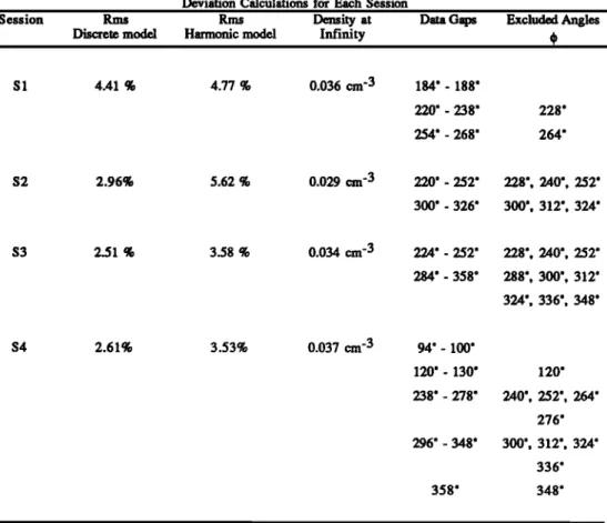
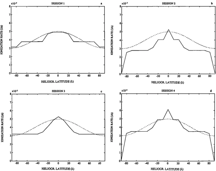
distributions for each session are shown in Figure 3 together with the harmonic ionization rate. Figure 4 shows the corresponding intensities and the measured intensity data. A

discussion of each session follows and in conclusion their

common features are studied. Rms (root mean square) values, densities at infinity, data gaps, and measuring angles •, which were excluded when calculating the standard deviation for each

session, are shown in Table 1.

The different densities at infinity listed in the Table 1 are calculated for the discrete model only. The corresponding values for the harmonic ionization rate range from 0.036 to 0.14. Thus the relatively good rms values in the case of the

harmonic model does not reflect the whole truth. However, we

wanted to compare the best results achieved using two different

models.

Since the ecliptic longitude for the session S1 was 11 ø, the measuring circle covers lines of sights toward both the upwind (• -- 350 ø- 20 ø, see Figure 4a) and the downwind direction (• -- 170 ø- 200 ø, see Figure 4a). The rms value for the discrete model

is the worst of all sessions, and there is a visible difference

between the data and the model around • = 0 ø - 70 ø (see Figure 4a). Thus this difference cannot be removed through simply changing the ionization rate. However, we do not exclude the possibility, that changing other parameters (such as velocity and temperature) would produce a better result. The multiple scattering is hardly responsible for these discrepancies, since according to Keller et al. [1981], the difference of the intensity between the upwind and downwind direction is overestimated in the optically thin model that we have used. As shown in Figure

4a, the difference between the upwind and the downwind

direction is underestimated by the model. It is also worth remembering that the velocity of the interstellar gas changes

while crossing the heliopause, and its effects are difficult to predict.

$UMMANEN ET AL.: LATITUDINAL DISTRIBUTION OF $OIJtR WIND 13,219

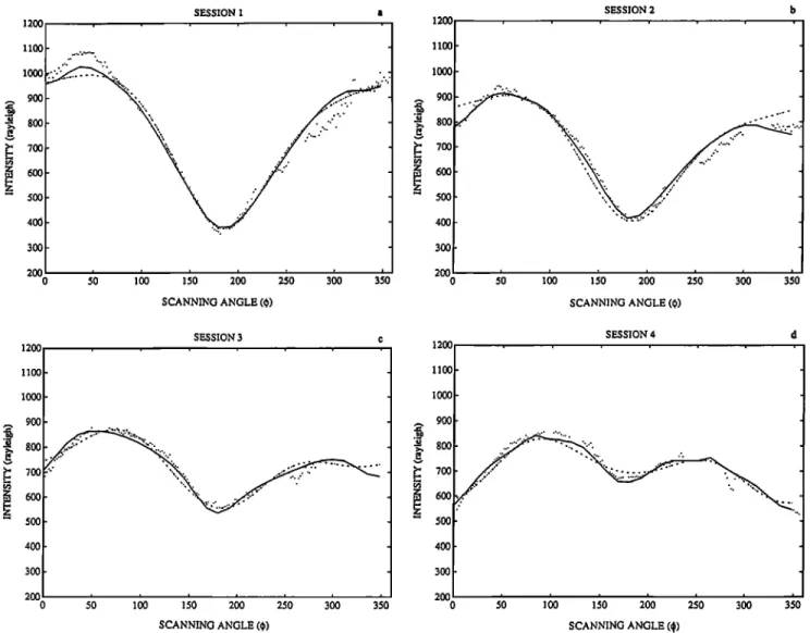
TABLE 1. Rms Values, Densities at Infinity, Data Gaps, and Angles • That Were Excluded in the Standard

Deviation Calculations for Each Session

Session Rms Rms Density at Data Gaps Excluded Angles

Discrete model Harmonic model Infinity •

S 1 4.41% 4.77 % 0.036 cm '3 184'- 188' 220' - 238' 254' - 268' 228' 264' S2 2.96% 5.62 % 0.029 cm '3 220' - 252' 300' - 326' 228', 240', 252' 300', 312', 324' S3 2.51% 3.58 % 0.034 cm '3 224' - 252' 284' - 358' 228', 240', 252' 288', 300', 312' 324', 336', 348' S4 2.61% 3.53% 0.037 cm '3 94' - 100' 120'- 130' 238' - 278' 296' - 348' 358' 120' 240', 252', 264' 276' 300', 312', 324' 336' 348'

TABLE 2. Parameter Values of the Interstellar Wind Used in Simulations Parameter Values T•o 8000 K IX 0.75 Wlo n 254.5' Wla t 6.0' v 0 20 km/s

Values are taken from Bertaax et al. [1985] and Dalaudier et al. [1984]. T, is the temperature of the hydrogen gas at infinity, ix is the radiation pressure divided by the gravitational

force, v 0 is the bulk velocity of the interstellar gas, and the wind directions Wlo n and wla t are the longitudinal and the

latitudinal angles in the ecliptic coordinate system.

The model results fit the intensity data well in the session S2. Six angles had to be excluded because of data gaps when calculating rms values. This could be the reason for the most striking feature in the discrete ionization rate distribution: the sudden decrease of the ionization rate near the poles. The rms value for the distribution, where the ionization rate at the poles

is assumed

to be the same

as at • = :k 80

ø (2.6x10

'7 s

'1 in

session S2), is 3.00%. Thus the difference of the rms values is less than 0.05%, and the deep slope near the poles is presumably an artificial feature, which reflects the great

uncertainty of the result near the poles. In session S3 the

fitting is mostly based on the data from the first half of the

measuring cycle, since there are two large data gaps around • =

224 ø - 252 ø and • = 284 ø - 358 ø.

The discrete ionization rate for the session S4

greatly resembles the ionization rate for the session S2. S4 and S2 share a sharp structure at the equator and a deep slope toward the zero at the poles. Because of these deep slopes, there are two sharp local maximum points in the intensity figure near • = 80 ø and • = 260 ø. If we straighten these slopes, the rms value would be 2.71%, and the sharp structures near the local maxima would disappear.

In each session there are two similar structures present. First,

there is an area of enhanced ionization near the equator. This

area covers the region from •, =-30 ø to •, = 30 ø. Second, there

are two broad plateaus from •, = +30ø to +70 ø. These

phenomena are quite possible if one considers the coronal structure of the Sun. According to solar observations, during the solar minimum, the large polar coronal holes reach to the low heliographic latitudes, and there is a narrow belt of slow solar wind, which lies along the equator. These phenomena seem to indicate more rapid change in the ionization rate near the equator, while the harmonic model predicts slower change.

On the other hand, the increase of the ionization toward the equator was already explained by the harmonic model.

Hydrogen atoms that scatter solar Lyman alpha radiation are exposed to the solar wind for several years, since their velocity

is only 4 AU in a year. The main contribution of the measured

intensity along the line of sight comes from the distance 5-10 AU that is, from the atoms, which have been influenced by the solar wind during the last 2-3 years. Thus the best ionization rate distribution is a kind of average over ionizing effects of

the Sun during the last two or three years. This is probably why

13,220 SUMMANEN Er AL.: LATITUDINAL DISTRIBUTION OF SOLAR WIND

x10 -? SESSION • , , . , ,

a

o

-;o

h

;o ;o ;o

-so -6o

o

60

HELIOGR. LATITUDE (t.) HELlOGR. LATITUDE (k)

xlo -? SESSION 2 b

2

x10'? SESSION 3 c x10'? SESSION 4 d

7

-80 -60 -40 -20 0 20 40 60 &0 -80 -60 -40 -20 0 20 40 60 HELlOGR. LATrrl. YDE (k) HELIOGR. LATITUDE (•.)

Fig. 3. The discrete ionization rate (solid line) and the harmonic ionization rate (dashed line) as a function of

the heliographie latitude I. for the session (a) S1, (b) S2, (e) S3, and (d) S4.

as -30 ø to 30 ø. The reason then for broad plateaus are the

coronal holes. The mean ionization rate calculated from four

sessions is shown in Figure 5. The common features explained above are clearly visible.

All results given above are calculated using fixed values of the interstellar wind parameters given in Table 2. Since there are so many variable parameters, the use of any other method based on the inversion theory was impossible. Also, the effect of varying the parameters could not be thoroughly tested. The

basic reason for this was the limited CPU time. Ionization rate

calculations required 300-1300 trials, until the best model was

found.

However, a few test runs were performed for the session S3. It

was chosen for its smooth latitudinal variations. The

ionization rate for the session S3 shown in Figure 3c was used as a starting point in these checking calculations. We changed the interstellar wind parameters, within the limits of error given by Lallement et al. [1985b] except the bulk velocity, which was changed by :k2 km/s. In checking runs, only one parameter was changed, while other parameters were kept fixed. In most of the test runs, the ionization rate changed very litfie. As a typical example of the changes, the ionization rate, when the temperature T is 10 000 K, is shown in Figure 6. Also, in the cases when T = 6000 K, p. = 0.65, p. = 0.85, the

longitude of the wind in ecliptic coordinates is 253 ø, the latitude is 4.5 ø, the bulk velocity v is 18 km/s or v is 22 km/s, the ionization rate deviated only slightly. However, when the longitude of the wind in ecliptic coordinates is 256 ø or the latitude is 7.5 ø, the level of the ionization rate changed considerably. As an example, the case when the latitude is 7.5 ø is shown in Figure 7. Thus the level of the ionization rate seems to vary when the interstellar parameters are changed, but

the common features, the enhanced ionization rate at the

equator and the plateaus at :!:30 ø to d:70 ø, remain unchanged in.

each of the test runs.

3.2. Estimated Latitudinal Variation of the Solar Wind Flux

If the ionization rate as a function of the heliographic

latitude is known, the latitudinal variation of the solar wind

proton flux (or solar wind proton density) can be calculated from (3). As an example of the derivation of the solar wind proton flux, the result of the session S3 is considered below.

Assuming

$UMMANEN ET AL.: LATITUDINAL DISTRIBUTION OF SOLAR WIND 13,221 120o SESSION 1 a 11oo 9• 800 400 300 200 20( 10( 00• 90• 80• 70• 600 500 4OO 300 0 SESSION 2 b ., ,io ,io

SCANNING ANGLE (•) SCANNING ANGLE (•)

1200 11oo iooo 9oo '-• 800 400 300 200 o SESSION 3 c ₁₂₀₍ SESSION 4 d 110( lOOC 8OO 500 3OO 20O 0 50 100 150 2•0 2;0 3•0 3;0 5• 160 1•'0 2•0 250 300 3;0 SCANNING ANGLE (qb) SCANNING ANGLE (•)

Fig. 4. The intensity

data

measured

during

the session

(a) S1, (b) S2, (c) S3, and

(d) S4 (dots)

and

calculated

intensities using the discrete ionization rate shown in Figure 3 (solid line) and the harmonic ionization rate (dashed line) as a function of the scanning angle •.

and

vrel(•.,r)=

Vpr(•.,r

) = vpr(•.

), we

have

[•(•) = n•r(•,)

r-•-m2

Vpr(•,)lo•(IVpr(•,)l)

+ [•ph(•,,r)

Vpr

= 350

km

s

'• + 800

sin2•.

km

s

'• , I•,1

_•

35

ø

Vpr----

600

km

s

'• , I•.1

> 35

ø

For the cross section an experimental expression by Fire et al.

[1962],

•oce

= 7.6x10

's- 1.06x10

's log•oE

(17)

is used. The cross section is given in units of square centimetres, and the energy of a proton, E, is expressed in

electron volts.

Kojima and Kakinuma [1990] have reviewed latitudinal

dependence of the solar wind as deduced from IPS measurements

and spacecraft measurements. They have listed three works, which concern the latitudinal dependence of the solar wind in

1976 and 1977. Here the results from Zhao and ttundhausen

[1981] (model 4 of Kojima and Kakinuma [1990]) are used. According to them there was a relationship between the solar

wind speed and the angular displacement •, from the neutral

sheet. The relationship in 1976 was estimated to be (see Figure

o

-io -;o

h

&

HELIOGR. LATITUDE (k)

Fig. 5. The mean ionization rate calculated from four sessions S1, S2, S3, and S4 as a function of the heliographic

13,222 SUMMANEN ET AL.: LATITUDINAL DISTRIBUTION OF SOLAR WIND x10-? 8 , 3 -•0 -•0 -;0 -•0 0 •0 ;0 sb HELIOGR. LATITU'DE (•.)

Fig. 6. The ionization rate as a fimction of the heliographic

latitude )• for the session S3 (dashed line), when the parameters.

are T = 10000 K, It = 0.75, the longitude of the wind in ecliptic

coordinates is 254,5 ø, the latitude is 6.0 ø and v = 20 lcm/s. The

ionization rate, when T = 8000 K (solid line), respectively.

HELlOGR. LATITUDE (3.)

Fig. 8. The latitudinal dependence of the solar wind velocity

as a function of the heliographic latitude •. in 1976 according

to Zhao and Hundha•en [ 1981].

In this work it is assumed,

that the angular

displacement

from the neutral sheet is approximately the same as the

heliographic latitude, also marked with •.. The corresponding

cross

sections

range

from

Oee(350

Inn

s

'l) = 2.140x10

'15

cm

2

to Oce(600

km s

'1) -- 1.705x10

'15

om

2.

Using

(16),

(17),

and

(18),

the

approximate

solar

wind

proton

flux

nvr(•,r)lVrel(•,r

) and

the

solar

wind

proton

density

can

be solved.

These

quantifies

for the session

S3 are

shown

in

Figure

9. The photoionization

is assumed

to be 0.88x10

'7 sq.

As shown

in Figure

9, the

solar

wind

proton

flux normalized

to 1 AU grows from 1.36x10

$ cm

-2 s

-1 at the poles

to

2.06x108

cm

'2 s

'1 at

the

equator,

that

is,

a growth

of 34%

in the

solar

wind

proton

flux

toward

the

equator.

This

is in agreement

with the values 25-35% given by Lallement et al. [1985b] using the harmonic model.

x10'? 8 ,

0 -•0 -•0 -•0 -•0

•

;0

40

60

8•

HELlOGR. LATITUDE (•.)

Fig. 7. The ionization rate as a function of the heliographic latitude )• for the session S3 (dashed line), when the parameters

are T = 8000 K, It = 0.75, the longitude of the wind in ecliptic

coordinates is 254,5 ø, the latitude 7.5 ø and v = 20 km/s. The ionization rate, when the latitude is 6.0 ø (solid line),

respectively.

o

o o

o

o o o o o

-do --•0 -;o -•o h do i0 6b HELIOGR. LATITUDE (3.)

xlO s

4 ,

o

o

o -•o -•0 -;o -3o o :o •0 60 sb ' HELIOGR. LATITUDE (•)

Fig. 9. The latitudinal dependence of the solar wind proton flux and density as a function of the heliographic latitude )• as

deduced from discrete ionization rate distribution for the session S3.

S-•N ET AL.: LATFFUDINAL DISTRIBUTION OF SOLAR WIND 13,223

However, it is worth noticing that the prediction about the solar wind proton flux is strongly dependent on the solar wind proton velocity model used. If two other model• for the year 1976 reviewed by Kojima and Kakinuma (models 5 and 6 used by Kojima and Kakinuma [1990, Table 1]) were used, the change in the solar wind proton flux at 1 AU would be 26% and

36-40% (different values in the velocity model for the north

and the south poles), respectively. The first of these two velocity models, model 5, is based on spacecraft observations, that were made in a narrow latitudinal range near the solar

equator. Thus the plateaus at high latitudes are missing. The

second velocity model, model 6, has lower plateaus than model

4 in Figure 8. In fact, both models 4 and 6 have quite smooth latitudinal gradient, IPS measurements during the next solar

cycle would prefer sharper gradient. These older models were

derived from the IPS data without considering the integration effect caused by the line-of-sight integrals, as pointed out by

Kojima and Kakinuma. However, in lack of better data, model 4 is used, since the plateaus are more pronounced there.

When the change of the solar wind proton flux from the plateaus to the equator is calculated using the ionization rate of another session, the session S4, the growth is about 28%. Thus the prediction by Lallement et al. (1985b) seems to be

reasonable.

Recently, Yang and Schunk [1991] have studied theoretically the latitudinal dynamics of steady solar wind flows beyond 0.15 AU. In their MHD simulations they have calculated the

latitudinal structure of the solar wind. Their results indicate the

existence of a proton number density maximum at the magnetic neutral line.

4. DISCUSSION AND CONCLUSIONS

The main results of this work are the following. First, it has

been shown that the intensities derived from the model best fit

the intensity data when the harmonic ionization rate is replaced

with a new distribution, where the enhanced ionization near the

solar equator and large plateaus around latitudes :t:30 ø - +_70 ø are

present. Second, it has been shown that the new ionization rate

distributions derived using the intensity data predicts 25-35% growth of the solar wind mass flux from the polar areas toward the equator as proposed by Lallement et al. [1985b].

The deep slopes of the ionization rate toward zero near the

poles that appear in the results of sessions S2 and S4 are very

likely artificial features. In fact, negative values of the ionization rate at •, = +_90 ø, would give still better rms values. However, any reliable physical model for the Sun would not produce negative ionization rate values. Thus the values of the ionization rates obtained here, which are around +-90 ø to +_70 ø , are highly questionable.

Although there is only a small difference in the rms values of

the calculated intensities between the harmonic model and the discrete models, there is a clear difference between the ionization rates. Also, it is shown that the best rms values,

which can be achieved using the symmetric ionization rate, are of the order 2.5%. This reflects partly the uncertainty of the method used to remove the contribution of the geocorona and partly, perhaps, the uncertain values of parameters. The geocorona had a considerable effect on data measured during the latter half cycle of the measuring circle.

The method that we have used is not precise enough to

predict the exact dependence of the solar wind proton flux on

the latitude. Because of the limited amount of computer time, the method could not be checked thoroughly. Also, the available latitudinal resolution is poor especially at high heliographic latitudes. Therefore the results near the poles and the width of the plateaus are questionable. One has to keep in mind that these solutions of this ill-conditioned problem are not necessarily the only possible solutions, and the method could have produced biased effects.

Also, when deriving the formulas for the density distribution and the optical model, several assumptions were made, the validity of which can be questioned. First, the flow of the

interstellar gas was considered as a stationary problem, although the solar wind and the EUV radiation are strongly

dependent on time [see Ajello et al., 1987]. This presumption was used when the equation of continuity was solved and when the ratio of the force on an atom due to radiation pressure to

that of gravity was assumed to be constant. Thus 27 day

variations caused by the rotation of the Sun as well as 11-year

cycles were neglected.

In the hot model it was assumed that the velocity distribution at infinity is Maxwellian; that is, the gas is in thermal equilibrium. To approach equilibrium, the nonuniformities of the temperature, density, and average velocity have to be smoothed out through collisions from one part of the gas to another. The average distance over which properties of the gas

can be transported in one elastic collision; that is, the mean

free

path

is approximately

llJ

17

m. It is of the

order

of parsecs

as the small structure of a diffuse interstellar cloud as given by

McKee and Ostriker [1977]. However, the thermalization of

neutral gas is possible also through elastic and charge

exchange collisions with other particle species. Thus the

Maxwellian distribution is reasonable.

It is also worth noticing that multiple scattering effects change the Lyman o• intensity distribution. The assumption of the optically thin medium underestimates the radial sky background intensity by 5-35% depending upon the angle between the interstellar wind and the line of sight [see Keller et

al., 1981]. The study of this phenomenon in the case of

Prognoz data is in progress. The presumption concerning the shape of the solar Lyman a line have certainly visible effects on the results. On the other hand, only a part of the information is retained in the line-of-sight integration in the

intensity measurements (see section 3). Thus the results are always averages over a long time (2-3 years) and distance (1-12

AU).

Many minor effects were ignored too. For example, only the effect of the solar wind protons was taken into account, while

all other

species

were

forgotten.

Also,

the r '2 dependence

in the

If the interstellar parameters could be derived independently

and a large set of Lyman o• data were available, the method could be tested more thoroughly. Fortunately, this will come

true in 1995, when the SWAN (Solar Wind ANisotropies)

experiment onboard the SOHO satellite will start to measure

Lyman o• data. At the same time, Ulysses will be measuring the solar wind. Then Ulysses in situ helium measurements will give data concerning the interstellar wind parameters simultaneously with the solar wind experiments of the velocity and the density of the solar wind. Furthermore, the WIND mission will provide baseline ecliptic plane observations while Ulysses and SOHO observe the Sun. WIND will be

13,224 $UMMANEN ET At,.: LATITUDINAL DISTRIBIYrION OF SOLAR WIND

launched in summer 1993. Then the full testing of this method will be possible.

Finally, the ionization rate distribution proposed above, is probably the furthest limit, which can be achieved using a stationary model. More precise results require the use of a time- dependent model including multiple scattering effects, which is the next step in modeling the flow of the interstellar matter

into the heliosphere.

Acknowledgments. We would like to thank the referees for the careful examination of the manuscript and very useful comments.

The Editor thanks K. Richter and D. Judge for their assistance in evaluating this paper.

Aje!1o, $. M., A. I. Stewart, G. E. Thomas, and A. Graps, Solar cycle study of interplanetary Lyman-alpha variations: Pioneer Venus orbiter sky background results, A.vtrophys. J.,.717, 964, 1987.

Axford, W. I., The interaction of the solar wind with the interstellar reediron, in Solar w/nd, edited by C. P. Sonett, P. $. Coleman, Jr., and $. M. Wilcox, NASA Spec. Publ. SP..?08, 609, 1972.

Axford, W. I., The solar wind, Sol. Phys., 100, 575, 1985.

Baranov, V. B., Gas dynamics of the solar wind interaction with the interstellar medium, Space Sci. Rev, 52, 89, 1990.

Bertaux, J. L., R. Lallemont, V. G. Kurt, and E. N. Mironova, Characteristics of the local interstellar hydrogen determined from Prognoz 5 and 6 interplanetary Lyman a profile measurements with a

hydrogen absorption cell, Astron. Astrophys., 150, 1, 1985.

Blum, P. W., and H. J. Fahr, Interaction between interstellar hydrogen and the solar wind, Astron. Astrophys., 4, 280, 1970.

Brandt, $. C., and Chamberlain, J. W., Interplanetary gas, I, Hydrogen

radiation in the night sky, Astrophys. J., 130, 670, 1959.

Chamberlain, $. W., Calculation of polarization and anisotropy of resonant and fluorescent scauering, learus, 84, 106, 1990.

Chamberlain, $. W., and D. M. Hunten, Theory of Planetary Atmospheres, An Introduction to Their Physics and Chemistry, pp. 290- 302, 2nd ed., Academic, San Diego, Calif., 1987.

Coles, W. A., and B. $. Rickett, IPS observations of the solar wind speed out of the ecliptic, J. Geophys. Res., 81, 4797, 1976.

Dalaudier, F., $. L. Bertaux, V. G. Kurt, and E. N. Mironova, Characteristics of interstellar helium observed with Prognoz 6 58.4-nm photometers, Astron. Astrophys., 1.74, 171, 1984.

Fahr, H. $., On the influence of neutral interstellar matter on the upper atmosphere, Astphys. Space Sci., 2, 474, 1968.

Holzer, T. E., Interaction between the solar wind and the interstellar medium, Ann. Rev. Astron. Astrophys., 27, 199, 1989.

Isenberg, P. A., and E. H. Levy, Polar enhancements of interplanetary La through solar wind asymmetries, Astrophys. $., 219, L59, 1978. Johnson, H. E., Backscatter of solar resonance radiation, I, Planet. Space

Sci., 20, 829, 1972.

$oselyn, $. A., and T. E. Holzer, The effect of asymmetric solar wind on the Lyman a sky background, $. Geophys. Res. 80, 903, 1975. Keller, H. U., K. Richter, and G. E. Thomas, Multiple scauering of solar

resonance radiation in the nearby interstellar medium, H, Astron. Astrophys., 102, 415, 1981.

Kojima, M., and T. Kakinuma, Solar wind speed, Space Sci. Rev., 5.?, 173, 1990.

Kumar, S., and A. L. Broadfoot, Evidence from Mariner 10 of solar wind flux depletion at high ecliptic latitudes, Astron. Astrophys., 69, LS-LS,

1978.

Kumar, S., and A. I.. Broadfoot, Signatures of solar wind latitudinal structure in interplanetary Lyman a emissions: Mariner 10 observations, Astrophys. J., 228, 302, 1979.

Lallement, R., $. L. Bertaux, V. G. Kurt, and E. N. Mirenova, Observed perturbations of the velocity distribution of interstellar hydrogen atoms in the solar system with Prognoz Lyman alpha measurements, Astron. Astrophys, 140, 243, 1984.

Lallement• R., $. L. Bertaux, and F. Dalaudier, Interplanetary Lyman a spectral profiles and intensities for both repulsive and attractive solar force fields: Predicted absorption pattern by a hydrogen cell, Astron. Astrophys., 150, 21, 1985a.

Lallement, R., $. D Bertaux, and V. G. Kurt, Solar wind decrease at high heliographic latitudes detected from Prognoz interplanetary Lyman alpha mapping, J. Geophys. Res., 90, 1413, 1985b.

Lee, M. A., The solar wind terminal shock and the heliosphere beyond, in Solar Wind Six Tech. Note, NCAR/TN..?O6+Proc., 635, Natl. Cent. for Atmos. Res., Boulder, Colo., 1988.

Lemaire, P., $. Charra, A. $ouchoux, A. V idal-Madjar, G. E. Artruer, $. C. Vial, R. M. Bonnett, and A. Skumanich, Calibrated full disk solar H I Lyman a and Lyman [• profiles, Astron. Astrophys., 22.?, I.•5, 1978. McKee, C. F,. and $. P. Ostriker, A theory of the interstellar medium:

three components regulated by supernova explosions in an inhomogeneous substrate, Astrophys. J., 218, 148, 1977.

Smith, E. $., and A. Barnes, Spatial dependences in.the distant solar wind: Pioneers 10 and 11, in Solar Wind Five, NASA Conf. Publ. 2280, 521,

1983.

Suess, S. T, The heliopause, Rev. Geophys., 28, 1, 97, 1990.

Summanen, T., Latitudinal distribution of solar wind as deduced from Lyman alpha measurements, Lic. thesis, Univ. of Helsinki, 1992. Weissbluth, M., Atoms and molecules, p. 516, Academic, San Diego,

Calif., 1978.

Witt, N., $. M. Ajello, and P. W. Blum, Solar wind latitudinal variations

deduced from Mariner 10 interplanetary H (1216 •)observations,

Astron. Astrophys., 7.?, 272, 1979.

Witt, N., $. M. Ajello, and P. W. Blum, Polar solar wind and interstellar wind properties from interplanetary Lyman-a radiation measurements, Astron. Astrop•s., 95, 80, 1981.

Yang, W.-H., and R. W. Schunk, Latitudinal dynamics of steady solar

wind flows i Astrophys. J., .?72, 703, 1991.

Zhao, X.-P,. and A. $. Hundhausen, Organization of solar wind plasma properties in a tilted, heliomagnetic coordinate system, J. Geephys. Res., 86, 5423, 1981.

$. L. Bertaux and R. Lallement, Service d'Aeronomie du Centre National de la Recherche Scientifique, F-91310 Verrilres-le-Buisson,

France.

E. Kyr61ii and T. Summanen, Finnish Meteorological Institute, P.O. Box 503, 00101 Helsinki, Finland.

(Received August 8, 1992; revised January 8, 1993; accepted January 12, 1993.)