HAL Id: hal-01072124
https://hal.archives-ouvertes.fr/hal-01072124
Submitted on 31 Mar 2016
HAL is a multi-disciplinary open access
archive for the deposit and dissemination of
sci-entific research documents, whether they are
pub-lished or not. The documents may come from
teaching and research institutions in France or
abroad, or from public or private research centers.
L’archive ouverte pluridisciplinaire HAL, est
destinée au dépôt et à la diffusion de documents
scientifiques de niveau recherche, publiés ou non,
émanant des établissements d’enseignement et de
recherche français ou étrangers, des laboratoires
publics ou privés.
Eric Quémerais, Bill Mcclintock, Greg Holsclaw, Olga Katushkina, Vlad
Izmodenov
To cite this version:
Eric Quémerais, Bill Mcclintock, Greg Holsclaw, Olga Katushkina, Vlad Izmodenov. Hydrogen atoms
in the inner heliosphere: SWAN-SOHO and MASCS-MESSENGER observations. Journal of
Geo-physical Research Space Physics, American GeoGeo-physical Union/Wiley, 2014, 119 (10), pp.8017-8029.
�10.1002/2014JA019761�. �hal-01072124�
RESEARCH ARTICLE
10.1002/2014JA019761
Key Points:
• Hydrogen atoms can reach the inner heliosphere
• Observed emission is compatible with models for solar minimum conditions • Mutual observations are very
effective to cross-calibrate two UV instruments
Correspondence to: E. Quémerais,
Citation:
Quémerais, E., B. McClintock, G. Holsclaw, O. Katushkina, and V. Izmodenov (2014), Hydrogen atoms in the inner heliosphere: SWAN-SOHO and MASCS-MESSENGER observations, J. Geophys. Res. Space Physics, 119, 8017–8029, doi:10.1002/2014JA019761.
Received 6 JAN 2014 Accepted 1 OCT 2014
Accepted article online 4 OCT 2014 Published online 29 OCT 2014
This is an open access article under the terms of the Creative Commons Attribution-NonCommercial-NoDerivs License, which permits use and distri-bution in any medium, provided the original work is properly cited, the use is non-commercial and no mod-ifications or adaptations are made.
Hydrogen atoms in the inner heliosphere: SWAN-SOHO
and MASCS-MESSENGER observations
Eric Quémerais1, Bill McClintock2, Greg Holsclaw2, Olga Katushkina3, and Vlad Izmodenov3,4,5
1LATMOS-OVSQ, Université Versailles Saint-Quentin, Guyancourt, France,2LASP, University of Colorado Boulder, Boulder,
Colorado, USA,3Space Research Institute, Moscow, Russia,4IPMech Institute for Problems in Mechanics, Moscow, Russia, 5MSU Lomonosov Moscow State University, Moscow, Russia
Abstract
We present here a study made by two instruments, Mercury Atmospheric and Surface Composition Spectrometer (MASCS) on MErcury Surface, Space ENvironment, GEochemistry, and Ranging (MESSENGER) and Solar Wind Anisotropy (SWAN) on SOHO that observed the interplanetary background in 2010. The combination of these two data sets allows us to perform the first study of the distribution of hydrogen atoms inside the Earth’s orbit. Triangulation of the position of the maximum emissivity region (MER) was performed for the data of the Ultraviolet and Visible Spectrometer (UVVS) channel of the MASCS-MESSENGER instrument. We find that the ecliptic longitude of the MER is 253.2◦± 2.0◦. This is the same value that was found from the analysis of the SWAN-SOHO H cell data obtained in 1996. This strongly suggests that the direction of the interstellar hydrogen wind has not changed between 1996 and 2010. We have also determined the distance of the MER to the Sun. We find that the volume emission rate peaks at 2.37 AU ± 0.2 AU from the Sun. This value is a good test for the solar parameters for total H ionization and radiation pressure used in models. Comparison between the two data sets obtained by the UVVS-MASCS channel and SWAN on SOHO allow to derive the intensity between the two spacecraft at peak emission. Based on the SWAN-SOHO calibration, we find an intensity of 80 R ± 36 R. This corresponds to a column density of 1540 m−3AU × 2.3 × 1014m−2. When divided by the distance between the two spacecraft,we find an average number density of 2300 m−3.
1. Introduction
The interplanetary background emission was first observed in the UV (H Lyman𝛼) at the end of the 1960s by the OGO-5 mission [Bertaux and Blamont, 1971; Thomas and Krassa, 1971]. While observing the hydro-gen exosphere of the Earth, the authors noticed an external component. This ubiquitous emission is due to the scattering of solar photons by hydrogen atoms present in the interplanetary medium. The interaction between the solar wind and interstellar hydrogen was initially studied by Blum and Fahr [1970].
The main component of the Lyman𝛼 background corresponds to the resonance scattering of the solar H Lyman𝛼 line. A similar background is caused by resonance scattering by helium atoms of the 58.4 nm solar line. Many UV instruments aboard planetary missions have been able to observe this emission [see
Ajello et al., 1987]. Recently, Quémerais et al. [2013] have tried to obtain a comprehensive view of the
inter-planetary background from the inner heliosphere to the outer heliosphere by combining various data sets (Voyager-ultraviolet spectrometer, SOHO-SWAN, Hubble Space Telescope-Space Telescope Imaging Spectrograph, and New Horizons-ALICE).
One application of the study of the interplanetary background is to derive information on the local inter-stellar medium (LISM) environment of the solar system. The hydrogen atoms that are observed in the interplanetary medium are one component of the interstellar cloud in which the solar system is currently traveling. The motion of the Sun with respect to the rest frame of the local cloud creates a flow of neu-tral atoms originating from the so-called upwind region that is defined by the relative velocity vector between the Sun and the local cloud. Therefore, the parameters of the hydrogen flow that are reflected in the interplanetary medium atom distributions are defined by the parameters of the local cloud. The case of hydrogen is complicated by charge exchange processes between neutral hydrogen atoms and protons in the solar wind and in the interface region between the solar wind and the ionized component of the local cloud [Baranov and Malama, 1993]. On the other hand, helium atoms are not very much affected by charge exchange and are used to characterize the parameters of the LISM [Möbius et al., 2004].
Recent observations by the Interstellar Boundary Explorer (IBEX) mission [Bzowski et al., 2012; Möbius et al., 2012] have suggested that previous estimates of the relative velocity vector between the solar system and the LISM cloud should be reevaluated. The IBEX findings give a slightly different direction and velocity com-pared to earlier results [Witte, 2004]. Similarly, the Voyager 1 spacecraft is now reaching the outer limits of the heliosphere and should soon be able to provide in situ measurements of the conditions outside of the heliosphere.
The aim of this paper is to detail observations made by two UV instruments in the inner heliosphere: the Ultraviolet-Visible Spectrometer (UVVS) during the cruise of the MErcury Surface, Space ENvironment, GEochemistry, and Ranging (MESSENGER) spacecraft to Mercury and the Solar Wind Anisotropy (SWAN) photometer on the SOHO mission at the L1 Lagrange point. By combining these two data sets we are able to derive column densities between the two spacecraft and therefore test models of the distribution of hydro-gen in the close vicinity of the Sun. In the following sections, we will detail the observations and models used in this study.
2. Data Sets
This section presents the two data sets that are used in this study.
2.1. UVVS-MASCS on the MESSENGER Spacecraft
The Mercury Atmospheric and Surface Composition Spectrometer (MASCS) instrument on MESSENGER consists of an Ultraviolet-Visible Spectrometer (UVVS) and a Visible-Infrared Spectrograph (VIRS). UVVS covers the wavelength ranges of the far ultraviolet (115–180 nm), middle ultraviolet (160–320 nm), and visible (250–600 nm), with an average spectral resolution of 0.3, 0.7, and 0.6 nm, respectively [McClintock
and Lankton, 2007]. UVVS uses an entrance slit with a field of view of 1◦by 0.04◦for its airglow studies. MASCS UVVS has been studying Mercury’s exosphere and surface reflectance properties initially from flyby observations [McClintock et al., 2008] and more recently from orbit.
The radiometric sensitivity of the far ultraviolet (FUV) channel of MASCS was determined prior to the launch of the MESSENGER spacecraft. Measurements were conducted in vacuum by observing the output from a monochromator with both MASCS and a photomultiplier detector, which itself was calibrated against a National Institute of Science and Technology photodiode. Flight observations of stellar sources provide an opportunity to validate the MASCS radiometric calibration. An adjustment of approximately 20% was applied to the MASCS spectral sensitivity in order to provide agreement with the Solar Radiation and Climate Experiment satellite SOLar STellar Irradiance Comparison Experiment-measured irradiance of the star Alpha Virginis (Spica) in the wavelength range 130–190 nm [Snow et al., 2013] and near Lyman𝛼 (M. A. Snow, private communication, 2012).
After launch on 3 August 2004, MESSENGER had an extended cruise phase of its mission in the inner helio-sphere until its orbital insertion at Mercury on 18 March 2011. During part of the cruise phase, in 2009–2011, Lyman𝛼 observations were obtained by UVVS over great circles as the spacecraft rolled at roughly right angles to the spacecraft-Sun line at distances from the Sun ranging from 0.30 to 0.57 astronomical units (AU). Because UVVS is a spectrometer, it is possible to separate the spectrum into heliospheric Lyman𝛼 emissions (excess counts within 0.3 nm of the Lyman𝛼 121.6 nm emission) and longer-wavelength starlight. By combining these observations, a Lyman𝛼 map of the full sky was obtained.
2.2. SWAN on the SOHO Spacecraft
The SOHO mission was launched in December 1995. This mission is a cooperation between European Space Agency (ESA) and NASA and is dedicated to the study of the Sun and its environment. While the main mission was intended to last 2 years (1996 to 1998), many of the SOHO instruments are still active in 2014. The SWAN instrument (Solar Wind Anisotropy) is a Lyman𝛼 photometer developed in cooperation between France (Service d’Aeronomie, CNRS) and Finland (Finnish Meteorological Institute, Helsinki) [Bertaux et al., 1995]. The SWAN experiment is composed of two identical units containing a periscope system, a hydrogen cell and an intensified anode detector with a CsI photocathode. Thanks to its periscope systems, the SWAN units can point in almost any direction that is not blocked by the spacecraft. The units are placed on oppo-site sides of the SOHO spacecraft, and data can be combined to cover all directions in the sky. A complete observation of the sky is performed in roughly 24 h.
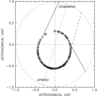
Figure 1. Mutual observation geometry between SOHO and
MESSENGER. The plot shows the position of the spacecraft in the ecliptic plane; the Sun is at the center. TheXandYaxes are distances in AU. The diamonds show the position of MESSEN-GER for each of the 143 rolls. The dotted circle shows the trace of the orbit of SOHO around the Sun. The solid lines are the two examples of mutual observations when SOHO is behind MES-SENGER. The dashed line shows the case when SOHO is ahead of MESSENGER. The thin dotted line shows the projection of the interstellar wind axis onto the ecliptic plane.
One of the science objectives of SWAN is to derive the pattern of the solar wind mass flux and its variations. SWAN records full sky maps of backscattered Lyman𝛼 intensity (i.e., inter-planetary background) on a daily basis. These maps are used to determine the distribution of interplanetary hydrogen atoms [Bertaux et al., 1995, 1997; Quémerais et al., 2006]. Based on comparisons between data and models of the interplanetary hydrogen distribution, the maps are used to derive the heliographic lati-tudinal distribution of the ionizing fluxes from the Sun. In the inner heliosphere, hydrogen atoms are ionized through charge exchange or photoionization processes. The main con-tributor is charge exchange between hydrogen atoms and solar wind protons. The charge exchange rate is equal to the product of the velocity-dependent cross section by the solar wind mass flux. Therefore, these measurements can be used to derive solar wind mass flux distributions and their temporal and spatial variations. Steps of the inversion scheme are detailed in Quémerais et al. [2006].
The SWAN instrument calibration is detailed in Quémerais et al. ([2013] International Space Science Institute (ISSI)). The units were not accurately calibrated on the ground, and the absolute calibration was obtained by comparison with measurements of the interplanetary background made by the Hubble Space Telescope in 1996 and 2001 when SWAN was looking in the same direction at the same time. Both SWAN units are intercompared on a daily basis because they can be pointed to the same area of the sky close to the ecliptic plane. This ensures an accurate tracking of the cross calibration of the two units. Temporal variations of the SWAN unit calibration factors are tracked by looking at stars on a regular basis (weekly basis before 2003 and daily basis since 2003).
Since 2007, SWAN has been performing full sky observations everyday. Before that period, full sky obser-vations were performed every other day with special obserobser-vations in-between, like dedicated comet observations, for example. At the time of the mutual observations with UVVS during the MESSENGER cruise, SWAN was performing daily observations with a few gaps caused by spacecraft maneuvers.
For the present analysis, we encountered a difficulty due to the fact the SWAN maps have gaps of spatial coverage close to the ecliptic plane. The first gap is due to the fact that SWAN cannot look close to the Sun which is too bright. Direct sunlight on the photocathode of the intensifiers would damage the detectors permanently. Therefore, the look direction of the unit must be kept at an angle larger than 10◦from the Sun. To prevent accidental observations, the direction of the Sun is blocked by an external occultor that blocks the SWAN unit field of views. Unfortunately, grazing sunlight on the edge of the occultors also cause some straylight within 15–20◦of the solar direction. On the antisolar direction, a large portion of the sky is blocked by the SOHO spacecraft. Reflected sunlight on the spacecraft also causes some straylight within a
Table 1. True Mutual Observations Between SOHO and MESSENGER
Roll Number Date of Observationa MESSENGER Longitude SOHO Longitude Delay in Days
37 2010/08/08 25.4943 315.665 1.19238
92 2010/11/12 342.867 48.1157 3.06836
108 2010/12/13 152.688 84.1970 2.57373
(a)
(b)
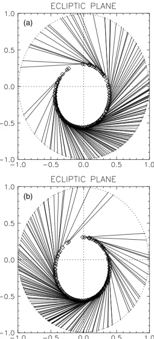
Figure 2. Delayed mutual observation geometry between
SOHO and MESSENGER. The plots show all existing rolls and the position of both spacecraft. (a) For UVVS looking ahead toward SOHO and (b) for UVVS looking behind toward SOHO.
few degrees from the blocked portion of the sky. When data necessary for our analysis were missing because of the gaps in the SWAN maps, we have interpolated the maps using inter-planetary background models. More details are given below.
3. Mutual Observations
The work presented here is based on the analy-sis of mutual observations performed between SWAN on SOHO and UVVS on MESSENGER during the MESSENGER cruise to Mercury in 2010 and 2011. These observations were purely serendipitous and were made possible by the fact that MESSENGER was rolling around its axis toward the Sun while SWAN was covering the entire sky.
Mutual observations between two UV instru-ments measuring the interplanetary back-ground on two different spacecraft can be used to cross-calibrate the two instruments. It also allows us to derive the intensity between the two spacecraft. Such observations were per-formed by the two Voyager spacecraft, and the results are presented in Hall [1992].
The basic concept is illustrated in Figure 1. Assume two spacecraft, S1and S2in the
helio-sphere, are able to measure the backscattered Lyman𝛼 emission. The mutual observation is achieved when both instruments record the Lyman𝛼 intensity in the interplanetary medium when looking toward the other spacecraft and in the opposite direction. If the column den-sity of hydrogen between the two spacecraft is small, so that it can be considered optically thin, then the sum of the two intensities mea-sured by each spacecraft should be the same. We can note the intensity measured by space-craft Siwhen looking toward Sjas I(i,j)and then the intensity measured by Siwhen looking in the direction opposite to Sjas I(i,−j). In that case we can show that, because extinction between S1and S2is negligible, we have
I(1,2)+ I(1,−2)= I(2,1)+ I(2,−1) (1)
The validity of equation (1) can be shown by considering the computation of the background intensity along the line of sight from S1looking toward S2. The intensity is the integral of the volume emission rate multiplied by the extinction between the observer (S1) and the scattering point of the photons [see, for instance, Quémerais, 2000]. This term takes into account the angle dependence of the phase function of the resonance scattering [see Quémerais, 2000]. When the medium is optically thin, the emissivity term, i.e., the density multiplied by the excitation rate, must be multiplied by the phase function term. Let us introduce the intensity observed by S1emitted between S1and S2. Here the integration over the line
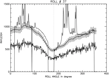
Figure 3. Comparison of the data of a roll (#37). The intensities are
plot-ted as a function of the angle of the line of sight with the ecliptic plane. An angle of 90◦points to North Ecliptic. The SWAN data are shown by the top curve with spikes corresponding to stars in the field of view. The bottom curves show the UVVS data with no stellar contamination. The noisy curve corresponds to raw data and the smooth curve to the smoothed data. The thick line shows the same UVVS data scaled by the factor 1.39 explained in the next figure. The corresponding error bars have been added to the scaled UVVS curve.
of sight stops at S2. It is noted I
S2 S1and is expressed by IS2 S1= 1 4𝜋 ∫ S2 S1 𝜀(⃗r) ⋅ T(S1, r) ⋅ dr (2)
The term𝜀(⃗r) expresses the volume emission rate at point⃗r on the line of sight and T(S1, r) is the extinc-tion between the point⃗r and the observer S1. When the extinction
between S1and S2is negligible then
T(S1, r) = 1.
Because the extinction on the line of sight is negligible between S1and S2, then we can split the integral of inten-sity in two terms when computing the intensity recorded by S1when looking toward S2. The first term is the integral
between S1and S2, and the second term
is the integral starting at S2looking away
from S1. ∫ ∞ S1 𝜀(⃗r) ⋅ T(S1, r) ⋅ dr = ∫ S2 S1 𝜀(⃗r) ⋅ dr + ∫ ∞ S2 𝜀(⃗r) ⋅ T(S2, r) ⋅ dr (3)
For a point on the line of sight going from S1to S2and beyond S2, the extinction between S1and that point and the extinction between S2and that point are the same in this case. Note also that the phase function term is the same because it depends on the square of the cosine of the scattering angle. Therefore, from equation (3), we can write
I(1,2)= IS2
S1+ I(2,−1) (4)
I(2,1)= ISS12+ I(1,−2) (5)
IS2
S1= I(1,2)− I(2,−1)= I(2,1)− I(1,−2) (6) The last equality is equivalent to the statement that the sum of intensities of one spacecraft is equal to the sum of the other spacecraft as given by equation (1). Using this equality, it is therefore easy to cross-calibrate the two instruments by comparing the sum of the two intensities for the two spacecraft.
3.1. True Mutual Observations
Mutual observations are not always easy to perform between two spacecraft. The operational constraints do not always make such observations possible even if the spacecraft are at the correct position. In our study, MESSENGER was on its cruise to Mercury and performed three elliptical orbits linking Venus to Mer-cury. In the same time SOHO at roughly 1 AU from the Sun was on a nearly circular orbit around the Sun. The MASCS instrument could only observe during the MESSENGER cruise in a plane perpendicular to the Sun-MESSENGER line. This means that there are only two positions possible for other spacecraft such as SOHO in orbit around the Sun, one with a larger ecliptic longitude (called ahead or SOHO A) and one with a smaller ecliptic longitude (called behind or SOHO B). Of course, the probability that SOHO was at the right position at the right time was rather small. Figure 1 shows two examples of mutual observations between MESSENGER and SOHO when SOHO is behind. There was also one case when SOHO is ahead of MESSENGER. The correct geometry was obtained in the three cases shown in Table 1. For these cases, we have accepted that there may be up to 3 days between the MESSENGER observation and the SWAN observation.
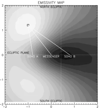
Figure 4. Explanation for the geometry of the observation in roll 37.
The contour plot shows the volume emission rate derived from the model in the plane perpendicular to the ecliptic plane and containing the line passing through the positions of SOHO and MESSENGER. The axes are distances in AU. TheXaxis is this line passing by the positions of MESSENGER and SOHO. In this case, SOHO is behind MESSENGER (SOHO B). The corresponding position of SOHO ahead of MESSENGER (SOHO A) is shown too. The point at (0,0) is the point of theXaxis clos-est to the Sun. The difference in intensities observed by SWAN and UVVS outside the ecliptic plane is caused by a parallax effect between MESSENGER and SOHO B. From this graph we see that SWAN measure-ments peak at lower latitude than UVVS measuremeasure-ments which is what is seen in the previous graph.
Because these observations are per-formed at the same time, it is not nec-essary to account for time-dependent effects in the interplanetary background. For delays more than a few days, it is nec-essary to correct for solar illumination variations because rotational modula-tions of the solar illuminating flux could induce variations up to 25% at Lyman
𝛼 during maximum solar activity [Pryor et al., 1992]. The observations studied
here were obtained in 2010 and 2011 during the ascending phase after the solar minimum in 2008.
3.2. Extension to Delayed Mutual Observations
Although the three true mutual obser-vations identified above are quite interesting because the results will be independent of any assumption con-cerning time-dependent effects, the number of mutual observations between SOHO and MESSENGER can be drasti-cally increased if we allow some delays between the observations by SWAN and MASCS. In this case, we can call them delayed mutual observations. In fact, for each roll performed by MESSEN-GER, there are always two points that cross the orbit of SOHO. In each case, we can compute the date when SOHO is at that position and choose the observa-tion which is closest in time to minimize effects of temporal variations of the interplanetary background. The longest delay is 6 months since this is the maximum time between two positions on the 1 year orbit of SOHO.
Figure 2 shows the delayed mutual observations when SOHO is ahead and behind, respectively. During the 1 year orbit of SOHO, MESSENGER performs three orbits around the Sun. When combining both ahead and behind cases, we obtain a good coverage of almost all parts of the inner heliosphere.
4. Data Analysis
The data obtained with the MESSENGER rolls during the cruise to Mercury allow us to get a precise value of the cross-calibration factor between the two UV instruments. The first task is to extract the corresponding data from the data sets of the two instruments.
Figure 3 shows a typical example of the data. The measured brightness are plotted versus the angle of the line of sight with the ecliptic plane. The UVVS roll values are shown by the lower curve in the figure. The noisy line shows the original data corresponding to individual data points. We have also plotted the smoothed data. The smoothed curve of UVVS data was obtained by applying a gliding mean filter to the raw data. The width of that filter is 10◦wide. The UVVS data used here have no stellar contamination. The instrument is a spectrometer, and its spectral bandwidth at Lyman𝛼 is very narrow (about 1 nm). Therefore, only hot stars can produce a contribution. This contamination is easily removed from the roll data by filter-ing out any spike outside of the measurement scatter. Extraction of the mutual observation measurements is straightforward. The two values for the mutual observations correspond to angles of zero and 180◦.
Figure 5. Cross calibration of SWAN and UVVS-MASCS. The plot shows
the sum of in-ecliptic intensities for both spacecraft. The SWAN values are shown by triangles. The solid line shows the scaled UVVS values. The bottom line shows the result of the linear regression between SWAN and UVVS values. The cross-calibration factor between both instruments is 1.39±0.05 . The diamonds show the ratio between SWAN and UVVS. There is no temporal effect over the 1 year period of this study.
The SWAN data are shown by the top curve for the same roll angle values. These data are strongly affected by stel-lar light. This is due to two reasons. First, there is no spectral filter and the photometer bandpass is 115–160 nm. Although the pixel size projected on the sky is 1◦by 1◦, because of chromatic aberration created by the hydrogen cell in the optical path; around 150 nm, the spot size corresponding to a star can be as large as 2◦[Bertaux et al., 1995]. Consequently, the SWAN data often show stellar contamination mainly along the plane of the galaxy. Isolated stars can easily be removed, and the background level can be interpolated. Some areas along the galactic plane are too large to be interpolated accurately. The exam-ple shown in Figure 3 illustrates a good case when the gaps in SWAN data do not prevent the extraction of the relevant data for the mutual observations. Out of all the mutual observations, about a third have incomplete SWAN data rolls that could not be interpolated with confidence.
As explained in the previous section, we expect that the intensity recorded by both instruments in the eclip-tic plane are equal if the space between the two spacecraft is empty of hydrogen atoms. In such a case, it is clear that the UVVS channel data are too low or the SWAN data too high. The thick line shows the UVVS roll data multiplied by a factor of 1.39 so that the two instruments agree in the ecliptic plane. This coefficient will be justified in the next paragraph. We also note that the SWAN data are higher than the scaled UVVS data for roll angles between 90◦and 180◦. This is due to a parallax effect that is shown in Figure 4. That figure shows contour plots of the volume emission rate in a plane containing the SOHO-MESSENGER line and that
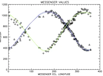
Figure 6. Values of intensities measured in the ecliptic plane by UVVS
as a function of the longitude of MESSENGER. The two curves corre-spond, respectively, to the ahead geometry case (triangle and blue) and the behind geometry case (diamond and green). The two curves are fits of the observations (see text). The residual scatter of the mea-surements from the fits is 20 Rayleigh. The ahead geometry data peak before the upwind longitude at 252◦. The behind geometry peaks after 252◦.
is perpendicular to the ecliptic plane (the normal vector of that plane is in the eclip-tic plane). Volume emission rate is equal to the density multiplied by the excitation rate which is proportional to the inverse square of the distance to the Sun. The intensity is the integral of the emission rate on the line of sight. At the time of observa-tion, there is more ionization in the ecliptic plane which is close to the solar equato-rial plane (7◦), causing the local maximum of volume emission rate to be split in two parts: one above the ecliptic plane and one below the ecliptic plane. These max-ima have an ecliptic longitude which is close to the longitude of the upwind direc-tion. Therefore, MESSENGER is closer to the Maxima than SOHO, which is in the SOHO B (behind) position. In that case, because of parallax, the maximum of intensity is seen by SWAN at a lower latitude than in the case of UVVS which explains why SWAN values are higher than UVVS values
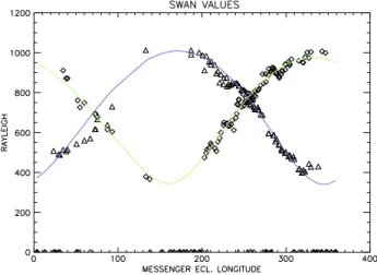
Figure 7. Values of intensities measured in the ecliptic plane by
SWAN as a function of the longitude of MESSENGER. The two curves correspond, respectively, to the ahead case (triangle and blue) and the behind case (diamond and green). The two curves are fits of the observations (see text). The residual scatter of the measurements from the fits is 30 Rayleigh. In the case of the SWAN, the data in the downwind region are rather sparse, but there are still some good observations that cross this region.
at midlatitude. If the maximum of volume emission rate had been at a low latitude, the effect would have been inverted and UVVS values at midlatitude would have been larger than SWAN values. The com-parison proves that the maximum of volume emission rate is close enough to create a parallax and that it is at midlat-itudes and not in the ecliptic plane. This constitutes a confirmation of an enhanced hydrogen ionization rate along the solar equator which lies close enough to the ecliptic plane.
4.1. Cross-Calibration Factor
The cross-calibration factor between SWAN and UVVS can be obtained rig-orously by using the sum of intensities obtained in the mutual observations (see equation (1)). A linear regression between the two data sets found a ratio of 1.39 ± 0.05. The values are shown in Figure 5. The two upper curves show the sums of inten-sities for both instruments. The solid line shows the UVVS-MASCS values multiplied by 1.39, and the triangles give the corresponding SWAN values. The bottom diamonds show the ratio between the actual data points. This is added to demonstrate that there is no pattern in the ratio. The straight line is the constant value of the cross-calibration factor at 1.39 . The ratio is constant over the whole period showing that there is no degradation of one of the instruments compared to the other.
Therefore, we can conclude that SWAN and UVVS measurements at Lyman𝛼 differ by a constant ratio of 1.39. This ratio is constant over the 1 year period considered.
4.2. Instrument Data Cross Comparison
Once the cross-calibration factor is computed, it is possible to compare the two data sets. Although the discrepancy between the two sets of measurements is large, almost 40%, it is a constant ratio over the whole data sets. On the one hand, the SWAN data have been compared to other measurements [see Quémerais
et al., 2013]. On the other hand, the UVVS channel calibration is pretty robust, as shown above. At the time
of writing, we cannot conclude on this matter. Future instrumentation like the PHEBUS instrument of the Bepi-Colombo mission [Chassefière et al., 2010] will bring new information on this matter.
For the present work, we can still obtain useful information about the hydrogen distribution in the inner heliosphere. Indeed, the question is to determine how much emission comes from between MESSENGER and SOHO. Since there is a constant factor between SWAN and UVVS data equal to 1.39, we have normalized the UVVS data to the SWAN calibration value. This choice is arbitrary and has been done for simplification. This will be discussed in section 6.
Figure 6 shows the UVVS measurements when the UVVS values have been multiplied by a factor of 1.39. The intensities are shown as a function of the ecliptic longitude of MESSENGER. There are two sets of values, one when UVVS is looking ahead (SOHO has a larger ecliptic longitude) and the other when UVVS is looking behind (SOHO has a smaller longitude). The two curves that fit the data (blue and green) correspond to the best numerical model given the measurement uncertainties. They were obtained by comparing the data with a radiative transfer model combined with a hot model of the hydrogen distribution [Quemerais, 2000]. Then, the residuals between model and data were fitted by a polynomial expression as a function of the intensity values. After the fit, there is no systematic bias remaining between the data and the fit. The remaining scatter between data and fit is 20 Rayleigh, corresponding to the measurement uncertainty. Figure 7 shows the SWAN data as a function of MESSENGER longitude. The intensities shown here are the values obtained when SWAN is looking away from MESSENGER. The two continuous curves correspond
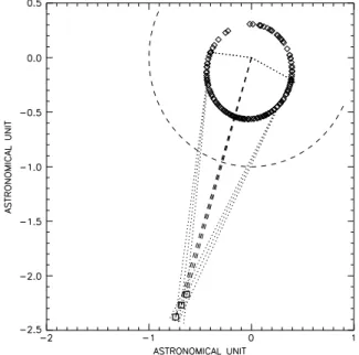
Figure 8. Triangulation of the position of the maximum
emissiv-ity region from the UVVS channel data in the ecliptic plane. The positions of the MESSENGER spacecraft are shown by the dia-monds. Each observation is made in the plane perpendicular to the MESSENGER-Sun line. The positions of the spacecraft for the two intensity peaks are shown. The MER is at the intersection of the two lines. The uncertainty is estimated by varying the positions by 2◦. The distance between the Sun and the MER is 2.37±0.2 AU. The ecliptic longitude of the MER is 253.2◦±2.0◦.
to numerical fit that represent the data within 30 Rayleigh and that were obtained in the same fashion as explained in the previous paragraph. As expected from the previous section, the SWAN measurements are systematically equal or lower than the MESSENGER values.
The ahead and behind observations from the UVVS channel can be used to triangu-late the position of the maximum emissivity
region in the ecliptic plane. From Figure 6,
we can derive the position of the maximum of intensity in both ahead and behind cases. From Figure 6, computing the derivative of the fit, we find that the peak intensity is reached when MESSENGER is at longi-tude 172.9◦. For the behind case the peak is reached for longitude 332.7◦. For these two observations, the distance between the Sun and MESSENGER is 0.40 AU for the ahead geometry and 0.44 AU for the behind geometry. Because of the geometry of the MESSENGER observations (rolls per-pendicular the Sun-MESSENGER line), the maximum emissivity region (MER) is at the intersection of the two lines perpendicular to the Sun-MESSENGER line in the ecliptic plane. The solution is found by searching the unique point of the first line that belongs to the second one. Figure 8 shows the geometry of the MER triangulation in the ecliptic plane. The value found for the distance between the MER and the Sun is 2.37 AU. The ecliptic longitude of the MER is 253.2◦.
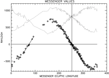
The values given above for the maximum intensity of the ahead and behind cases are model dependent. Therefore, to evaluate the accuracy of our determination of the direction of the interstellar hydrogen flow, we have used the following approach. First, we note that the two curves of the ahead and behind intensities have one crossing point in the upwind direction and one in the downwind direction. Each crossing point corresponds to the case when the difference of both intensities is equal to zero. Geometrically this happens when MESSENGER crosses the plane containing the wind axis and the vector perpendicular to the ecliptic plane. Figure 9 shows the two intensity curves ahead and behind. The diamonds show the difference. This difference becomes zero when the ecliptic longitude of MESSENGER is equal to the ecliptic longitude of the interstellar H flow. The ecliptic longitude of the H flow may be slightly offset but this is not the matter here. We want to determine the accuracy with which this longitude is determined and not the actual value which was already obtained above. This is done by a linear fit of the difference curve taking into account the statistical uncertainty. We used the algorithm given in numerical recipes (Press et al.) pages 655 to 657. The linear fits are shown in Figure 9. The linear fit of the difference is written as a + b⋅ l, where l is the longitude. If𝜎aand𝜎bare the uncertainties on coefficients a and b in the fit, and noting the longitude of the H flow as
LHand the corresponding uncertainty as𝜎H, then we have
LH= −a b (7) 𝜎2 H= 𝜎2 a b2 + a2𝜎2 b b4 (8)
The values shown in Figure 9 give a corresponding uncertainty of 2◦. The value found for the position of the MER gives an ecliptic longitude of the MER that is equal to the value found by Quemérais et al. [1999] from the analysis of the SWAN H cell data. These data were obtained in 1996 and 1997, while the MESSENGER
Figure 9. Difference of intensities measured in the ecliptic plane by
UVVS as a function of the longitude of MESSENGER. The two dotted lines at the top correspond to the data shown in the previous figure, the ahead geometry case and the behind geometry case. The dia-monds show the difference of the data sets and the corresponding error bars. The difference becomes zero once in the upwind direc-tion and once in the downwind direcdirec-tion. This corresponds to the positions when MESSENGER is closest to the wind axis. The ecliptic longitude of MESSENGER is determined by fitting a straight line to the data, and the corresponding uncertainty of 2◦is obtained from the result of the linear fit.
data have been obtained in 2010. This proves that over a period of 14 years, the direction of the hydrogen flow has not changed.
Based on the data shown in Figures 6 and 7, we can derive the intensity between SWAN and MESSENGER by substraction of the curves. When MESSENGER is in the down-wind cavity, the difference is equal to zero within the uncertainty of the data. Since this is obtained by a difference of two data sets, we estimate the uncertainty by taking the square root of the sum of the square of both uncertainties, which gives 36 Rayleigh. When MESSENGER peaks on the upwind side of the inner heliosphere, the maxi-mum intensity between the two spacecraft is equal to 80 ± 36 R. The peak intensity for UVVS is 1100 R, which means that the intensity between SWAN and MESSENGER corresponds to 7% of the total. If we apply the UVVS calibration, this value becomes 58 R ± 25 R. Transforming the intensity value into a column density is not straightforward because the solar flux varies over the line of sight and the derived value depends on the distance between the Sun and the scatter-ing atoms. However, a model comparison can give an estimate. This will be discussed in the next section.
5. Comparison to Model
Figure 10 displays a contour plot of the modeled volume emission rate (density divided by the square of the distance to the Sun) in the ecliptic plane. The Cartesian grid in the ecliptic plane is labeled in AU. The Sun position is at (0, 0), and the wind axis projection on the ecliptic plane is shown by the dashed line. The maximum of volume emission rate (MER) is shown by the bright region of the contour plot. The dark part extending in the downwind region is the downwind cavity which is empty of hydrogen atoms.
This model distribution is detailed in Izmodenov et al. [2013] and depends strongly on the solar parameters for total ionization rate of H atoms and on the radiation pressure coefficient. Increasing radiation pressure or total ionization increases the size of the cavity surrounding the Sun. This model corresponds to solar conditions derived in 2009 [Katushkina et al., 2013].
The orbit of SOHO is shown by the dotted line, and the MESSENGER cruise orbit is shown by the diamonds. Each diamond corresponds to one of the rolls used in this study. Two examples of mutual observations are shown in the plot. In one case (MESSENGER longitude is 25◦), the line of sight looking ahead goes through the cavity. For this line of sight both UVVS and SWAN will measure the same value. In the second case (MESSENGER longitude close to 190◦), the line of sight looking ahead goes through the maximum volume emission rate region. This will give a maximum intensity for both SWAN and UVVS, but UVVS will have an excess of 80 Rayleigh over SWAN. When looking ahead, the intensity peaks before MESSENGER reaches the upwind longitude, and when looking behind, the peak intensity is obtained for a longitude that is larger than the upwind longitude. The triangulation of the MER position for these two peaks was shown in the pre-vious section. We have compared this position to two models of the hydrogen atoms distributions described in Katushkina et al. [2013]. One was obtained for solar conditions in 2003 so after the solar maximum of 2001. The second distribution (shown in Figure 10) was computed for the solar conditions of 2009, so rather
Figure 10. Contours of the volume emission rate map in 2009 in the
ecliptic plane. The maximum of volume emission rate in the plane is shown by the white region and is aligned with the direction of the incoming interstellar wind. The orbit of SOHO is shown by the dotted line, and the MESSENGER position for the rolls is shown by the dia-monds. Two examples of mutual observations are shown. One of the examples shows a maximum of excess intensity for UVVS when the line of sight crosses the maximum of volume emission rate region at ecliptic longitude 253◦.
close to the time of the
MESSENGER-MASCS Interplanetary Hydrogen (IPH) rolls. The hydrogen interstellar wind direction in the model was chosen as 253.2◦. The results are summarized in Table 2. The “close to solar maximum” model for 2003 gives a MER-Sun distance equal to 2.2 AU which is close to the MASCS value. On the other hand, the model estimates the maximum intensity between SOHO and MESSEN-GER to be about 11 R when the data give 80 R. The second model for 2009 solar conditions gives an estimate of the maxi-mum intensity of 70 R which is very close to the data but gives a MER-Sun dis-tance equal to 1.4 AU which is too small compared to the MASCS value.
For each model we have esti-mated the column density (in units of m−3AU). The column
density is expressed in this unit because typical lengths are of the order of the astronomical unit. The values are shown in Table 2. From the geometry of
observation, we can compute the distance between SOHO and MESSENGER for the maximum intensity. The value is 0.68 AU.
The best model (2009) gives a SOHO-MESSENGER intensity of 70 R. If we correct for the actual value of 80 R, we get a column density of 1540 m−3AU. So the average density between SOHO and MESSENGER peaks
at 2300 m−3± 1000 m−3. Using the 2003 model gives a maximum column density only 20% larger. This
means that this derivation, although it is approximated, is not very sensitive to the actual hydrogen distri-bution model used. The peak intensity in the model must be scaled to the peak intensity between the two spacecraft derived from the data.
In conclusion, we have determined the distance between the Sun and the MER from the
MESSENGER-MASCS data. Comparison with hydrogen models derived for solar conditions in 2003 and 2009, respectively, shows that the best agreement is obtained for the conditions close to the solar maximum of 2003. This suggests that in the 2009 model the H atoms are too close to the Sun (1.4 AU) compared to the data. Therefore, in this model, either the ionization rate or the radiation pressure is not high enough. On the other hand, the 2009 model gives an estimate of the SOHO-MESSENGER peak intensity of 70 R, which is very close to the peak intensity in the data (80 R), deriving the corresponding column density is model dependent. The value found from the 2009 model divided by the SOHO-MESSENGER distance gives an average number density of hydrogen atoms between SOHO and MESSENGER of 2300 m−3± 1000 m−3.
This value is based on the SWAN calibration level. If we use the MASCS-UVVS calibration level, the value of the mean density is 1640 m−3± 700 m−3. Saul et al. [2012] have published values of the interplanetary
hydrogen seen by IBEX-Lo. To compare to our results, one would have to assume a velocity profile. A very simple calculation can be done by assuming an average velocity of 25 km s−1. In such a case, we get a flux of
5750 cm−2s−1. This value is larger, by a factor of 5 to 6, than the flux given in Figure 6 of Saul et al. [2012].
Table 2. True Mutual Observations Between SOHO and MESSENGER
MER Distance SWAN-SOHO Maximum Intensity Maximum Column Density
Data (2010) 2.37±0.12 AU 80±36 R
2003 Model 2.2 AU 11 R 260 m−3AU = 3.9×10¹³
When using the MASCS-UVVS calibration the ratio is decreased by a factor of 1.39. Given the simple calculation performed here, it would be best to do the actual modeling of the H distributions. This will be studied in future works.
6. Conclusion and Discussion
The data analysis presented here shows that the mutual observations are a very effective way to cross-calibrate two instruments at Lyman𝛼 even if their respective fields of view and spectral bandwidth are different. Indeed, SWAN is a photometer with a 110–160 nm bandwidth and with a 1◦by 1◦field of view, while UVVS is a grating spectrometer with a resolution of 0.3 nm and a field of view defined by a slit of 1◦ by 0.04◦.
We have shown that the necessity of performing the mutual observations at the same time can be allevi-ated if there are many observations and they are performed within 6 months of each other. In times of solar maximum, it is necessary to correct the data for solar flux variations. However, in the work presented here corrections for solar flux variations were not applied. We estimated the corrections based on solar Lyman
𝛼 flux measurements at the time our observations were made. We found that the corrections were always
smaller than 5 to 10% and could be neglected here.
When performing the cross calibration, we found that the ratio between the two data sets was very stable, with a mean value of 1.39 ± 0.05. A similar result was found by Pryor et al. [2013]. In this work, the authors scaled both data sets to a model and derived a cross-calibration ratio of 1.3. At the present time, it is not possible to clarify this matter any further but a similar topic was discussed at length by the Fully Online Database of UV Emissions (FONDUE) working group which was sponsored by ISSI (see Cross-Calibration of Far UV Spectra of Solar System Objects and the Heliosphere, ISSI Scientific Report Series, Volume 13. ISBN 978-1-4614-6383-2, editors E. Quémerais, M. Snow, and R.M. Bonnet, 2013).
The MESSENGER-MASCS data can also be used to triangulate the position of the maximum of volume emission rate (MER) in the interplanetary medium. This maximum is aligned with the direction of the inter-stellar hydrogen wind. Its ecliptic longitude (J2000) is equal to 253.2◦± 2.0◦. This value is very close to the one found by Quémerais et al. [1999] when analyzing the SWAN hydrogen cell data obtained in 1996 and 1997. This suggests that the interstellar hydrogen wind directions have been stable between 1996 and 2010. Recently, Frisch et al. [2014] suggested that the He interstellar wind may have been shifting in the last few decades. Our conclusion about interstellar hydrogen does not support this suggestion. If the claim of Frisch et al. [2014] is correct, it will be necessary to understand why the interstellar hydrogen direction seems stable.
In this work, we also find that at the time of IPH observations by MASCS in 2010, the MER is at 2.37 ± 0.2 AU from the Sun. This does not compare well to our current model for close to solar minimum conditions because it gives a MER-Sun distance equal to 1.4 AU. On the other hand, the model for close to solar maxi-mum conditions gives a distance of 2.2 AU. This would suggest that the in-ecliptic parameters are not large enough (radiation pressure or hydrogen total ionization). This will be studied in detail in future works with the SWAN data that can be used to get the MER position from parallax values and triangulation.
By comparison with models that propagate hydrogen atoms in the solar system [Izmodenov et al., 2013] and using time-dependent simulations to include the variations of the solar parameters for the solar wind and the radiation pressure, we find that the 80 Rayleigh emission observed between SOHO and MESSENGER is compatible with model predictions using solar parameters that correspond to close to solar minimum con-ditions. Similar computations for solar maximum conditions show that the model predicts that there will be almost no hydrogen atom within 1 AU from the Sun because of the combination of a larger radiation pressure and stronger ionization fluxes from the Sun. Based on this model and scaling to the actual value observed by the two instruments, we can derive the column density between SOHO and MESSENGER at the peak of emission, and knowing the distance, we can derive an average number density for interplanetary hydrogen. Finally, this can be compared to the interplanetary fluxes measured by IBEX and reported by Saul
et al. [2012]. Assuming an average H atoms velocity of 25 km s−1, we find a flux that is 4 to 6 times larger
than the one reported by Saul et al. [2012]. This last comparison is not very accurate as we simply multi-plied our number density by an average velocity and a more complete computation using an actual velocity distribution will be performed in a future work.
References
Ajello, J. M., A. I. Stewart, G. E. Thomas, and A. Graps (1987), The binary frequency of high-velocity field dwarfs as obtained with CCD measures, Astrophys. J., 317, 964–986.
Baranov, V. B., and Y. G. Malama (1993), Model of the solar wind interaction with the local interstellar medium - Numerical solution of self-consistent problem, J. Geophys. Res., 98(A9), 15,157–15,163.
Bertaux, J. L., and J. E. Blamont (1971), Evidence for a source of an extraterrestrial hydrogen Lyman-alpha emission, A & A, 11, 200. Bertaux, J. L., E. Kyrölä, E. Quémerais, R. Pellinen, R. Lallement, and W. Schmidt (1995), SWAN: A study of solar wind anisotropies on SOHO
with Lyman alpha sky mapping, Sol. Phys., 162(1–2), 403–439.
Bertaux, J. L., E. Quémerais, R. Lallement, E. Kyröelä, W. Schmidt, T. Summanen, J. P. Goutail, M. Berthe, J. Costa, and T. Holzer (1997), First results from SWAN Lyman a solar wind mapper on SOHO, Sol. Phys., 175(2), 737–770.
Blum, P. W., and H. J. Fahr (1970), Interaction between interstellar hydrogen and the solar wind, Astron. Astrophys., 4, 280–290. Bzowski, M., et al. (2012), Neutral Interstellar Helium Parameters Based on IBEX-Lo Observations and Test Particle Calculations, 12, vol. 198. Chassefière, E., et al. (2010), PHEBUS: A double ultraviolet spectrometer to observe Mercury’s exosphere, Planet. Space Sci., 58(1–2),
201–223.
Frisch, P., et al. (2014), Decades-long changes of the interstellar wind through our solar system, Sci. Mag., 341, 1080–1082. Hall, D. (1992), Ultraviolet resonance radiation and the structure of the heliosphere, PhD thesis, Ariz.
Izmodenov, V. V., O. A. Katushkina, E. Quémerais, and M. Bzowski (2013), Distribution of interstellar hydrogen atoms in the heliosphere and backscattered solar Lyman-𝛼, ISSI Scientific Report Series, vol. 13, Springer Science and Business Media, New York.
Katushkina, O. A., V. V. Izmodenov, E. Quemerais, and J. M. Sokol (2013), Heliolatitudinal and time variations of the solar wind mass flux: Inferences from the backscattered solar Lyman-alpha intensity maps, J. Geophys. Res. Space Physics, 118, 2800–2808, doi:10.1002/jgra.50303.
McClintock, W. E., and M. R. Lankton (2007), The Mercury Atmospheric and Surface Composition Spectrometer for the MESSENGER mission, Space Sci. Rev., 131, 481–521.
McClintock, W. E., E. T. Bradley, R. J. Vervack, R. M. Killen, A. L. Sprague, N. R. Izenberg, and S. C. Solomon (2008), Mercury’s exosphere: Observations during MESSENGER’s first Mercury flyby, Science, 321(5885), 92–94, doi:10.1126/science.1159467.
Möbius, E., et al. (2004), Synopsis of the interstellar He parameters from combined neutral gas, pickup ion and UV scattering observations and related consequences, Astron. Astrophys., 426, 897-907.
Möbius, E., et al. (2012), Interstellar gas flow parameters derived from Interstellar Boundary Explorer–Lo observations in 2009 and 2010: Analytical analysis, Astrophys. J. Suppl., 198(2), 11, doi:10.1088/0067-0049/198/2/11.
Pryor, W. R., J. M. Ajello, C. A. Barth, C. W. Hord, A. I. F. Stewart, K. E. Simmons, W. E. McClintock, B. R. Sandel, and D. E. Shemansky (1992), Astrophys. J., 394, 363–377.
Pryor, W. R., M. Snow, E. Quémerais, and S. Ferron (2013), Lyman-𝛼observations of comet Holmes from SORCE SOLSTICE and SOHO SWAN, in Cross-Calibration of Far UV Spectra of Solar System Objects and the Heliosphere, vol. 13, p. 255, Springer, New York. Quémerais, E. (2000), Angle dependent partial frequency redistribution in the interplanetary medium at Lyman alpha, A & A, 358,
353–367.
Quémerais, E., J.-L. Bertaux, R. Lallement, M. Berthé, E. Kyrölä, and W. Schmidt (1999), Interplanetary Lyman alpha line profiles derived from SWAN/SOHO hydrogen cell measurements: Full-sky velocity field, J. Geophys. Res., 104(A6), 12,585–12,604.
Quémerais, E., R. Lallement, S. Ferron, D. Koutroumpa, J.-L. Bertaux, E. Kyrölä, and W. Schmidt (2006), J. Geophys. Res., 111, A09114, doi:10.1029/2006JA011711.
Quémerais, E., B. R. Sandel, V. V. Izmodenov, and G. R. Gladstone (2013), Cross-Calibration of Far UV Spectra of Solar System Objects and the Heliosphere, ISSI Sci. Rep. Ser., vol. 13, edited by E. Quéémerais et al., pp.141–162, Springer, New York.
Saul, L., et al. (2012), Local interstellar neutral hydrogen sampled in-situ by IBEX, Astrophys. J. Suppl., 198 (2), 14, doi:10.1088/0067-0049/198/2/14.
Saul, L., M. Bzowski, S. Fuselier, M. Kubiak, D. McComas, E. Möbius, J. Sokół, D. Rodr´ıguez, J. Scheer, and P. Wurz (2013), Local interstellar hydrogen’s disappearance at 1 AU: Four years of IBEX in the rising solar cycle, Astrophys. J., 767(2), 130, doi:10.1088/0004-637X/767/2/130.
Snow, M., A. Reberac, E. Quémerais, J. Clarke, W. E. McClintock, and T. Woods (2013), A new catalog of ultraviolet stellar spectra for cali-bration, in Cross-Calibration of Far UV Spectra of Solar System Objects and the Heliosphere, ISSI Sci. Rep. Ser., SR-013, vol. 13, edited by E. Quémerais, M. Snow, and R. M. Bonnet, pp. 191, Springer, New York.
Thomas, G. E., and R. F. Krassa (1971), OGO 5 measurements of the Lyman alpha sky background, A & A, 11, 218.
Witte, M. (2004), Kinetic parameters of interstellar neutral helium: Review of results obtained during one solar cycle with the Ulysses/GAS-instrument, Astron. Astrophys., 426, 835–844.
Acknowledgments
SOHO is a mission of cooperation between ESA and NASA. SWAN was developed as a cooperation between France (CNRS, CNES) and Finland (Finnish Meteorological Institute). O.K. and V.I. were supported in part by RFBR grant 13-01-00265 and Presid-ium RAS program 22. Calculations of the interstellar hydrogen distri-butions were performed by using the supercomputers of Lomonosov Moscow State University (Lomonosov and Chebyshev).
Alan Rodger thanks Feze Arikan for his assistance in evaluating this paper.