HAL Id: hal-00958578
https://hal.archives-ouvertes.fr/hal-00958578
Submitted on 17 Mar 2014
HAL is a multi-disciplinary open access
archive for the deposit and dissemination of
sci-entific research documents, whether they are
pub-lished or not. The documents may come from
teaching and research institutions in France or
abroad, or from public or private research centers.
L’archive ouverte pluridisciplinaire HAL, est
destinée au dépôt et à la diffusion de documents
scientifiques de niveau recherche, publiés ou non,
émanant des établissements d’enseignement et de
recherche français ou étrangers, des laboratoires
publics ou privés.
On the calibration of a superconducting gravimeter
using absolute gravity measurements
Jacques Hinderer, Nicolas Florsch, J. Mäkinen, Hilaire Legros, J. E. Faller
To cite this version:
Jacques Hinderer, Nicolas Florsch, J. Mäkinen, Hilaire Legros, J. E. Faller. On the calibration of a
superconducting gravimeter using absolute gravity measurements. Geophysical Journal International,
Oxford University Press (OUP), 1991, p. 491-497. �10.1029/98GL00712�. �hal-00958578�
Geophys. J . Int. (1991) 106, 491-497
On the calibration of a superconducting gravimeter using absolute
gravity measurements
J.
Hinderer,' N. Florsch,2 J. M a k i ~ ~ e n , ~
H. Legros' and J.
E.
Faller4
'
Laboratoire de Giodynamique, Institut de Physique du Globe, 5 rue Renk Descartes, 67084 Strasbourg Cedex, France'
Laboratoire de Gkophysique Appliquke, Universiti P. et M . Curie, 4 place Jussieu, 75252 Paris Cedex 05, FranceFinnish Geodetic Institute, Ilrnalankatu l A , SF-00240 Helsinki, Finland
Joint Institute for Laboratory Astrophysics, University of Colorado, Boulder, CO 80309, USA
Accepted 1991 March 2. Received 1991 March 1; in original form 1990 October 23
S U M M A R Y
A 24 hr continuous parallel registration between an absolute free-fall gravimeter and a relative cryogenic gravimeter is analysed. Different adjustment procedures ( L , , L2
norms) are applied to the sets of absolute and relative readings in order to estimate the value of the calibration factor of the superconducting meter, as well as its uncertainty. In addition, a sensitivity test is performed to investigate the influence of some parameters (like the laser frequency and its short-term drift) upon this factor. The precision in the calibration factor is found to be better than 1 per cent, but systematic effects related to the short time interval may add another one and half per cent uncertainty. From preliminary results, it appears that this calibration experiment leads to a close agreement between the values of the gravimetric factor for the reference tidal wave O1 observed with the superconducting meter and the theoretical value (Dehant-Wahr body tide
+
ocean loading).Key words: absolute gravity, calibration, superconducting gravimeter.
1 I N T R O D U C T I O N
The problem of accurately calibrating a superconducting gravimeter is of fundamental importance for any geophysical interpretation of the high-quality data provided by this instrument (an accuracy of 0.1 per cent is required in tidal research). There are several well-known methods based on mass attraction or inertial acceleration (e.g. Van Ruymb- ecke 1989) that can be used to estimate the conversion factor (calibration) which transforms the 'gravity' output voltage (in Volts) from the feedback system of the relative meter in true gravity variations (in pgal). Usually, most of the relative meters (including the superconducting ones) are calibrated from the comparison with a parallel registration of another, or several other relative gravimeters which are themselves precisely calibrated on a calibration line (e.g. Wenzel, Zurn & Baker 1990). The tidal applications of absolute gravimeters were pointed out by Niebauer (1987). Using a 1 month series of absolute observations, he was able to determine the gravimetric factor at Boulder by comparing the absolute gravity record (corrected for air pressure and ocean loading) to theoretical tides. One can also use an absolute meter for calibrating a simultaneously recording tidal gravimeter; such an experiment was first performed by Wenzel (1988). We investigate here the possibility of
calibration of a superconducting gravimeter by using a parallel registration of a continuous set of 24 hr of absolute gravity observations made with a free-fall gravimeter. In Section 2, we briefly report on the gravimeters used in the experiment, and on the measurements. The results for the calibration factor (and its uncertainty) using different adjustment procedures (L, , L, norms) between absolute and relative readings are given in Section 3 and a sensitivity analysis is performed in Section 4 in order to see the influence of some parameters (frequency of laser and its temporal drift). We finally test the validity of the calibration factor by comparing the gravimetric factor for a reference
tidal wave observed with the superconducting meter and the theoretical value (Dehant-Wahr body tide
+
ocean load).2 D E S C R I P T I O N O F T H E E X P E R I M E N T 2.1 The absolute gravimeter
The absolute gravimeter (JILA-5) of the Finnish Geodetic Institute belongs to the series of six instruments built by J. E. Faller and his associates at the Joint Institute for Laboratory Astrophysics (JILA), National Institute of Standards and Technology and University of Colorado, Boulder (USA); for a detailed description, see Faller et al.
491
by guest on August 8, 2013
http://gji.oxfordjournals.org/
492 J. Hinderer et al.
(1983), Niebauer, Hoskins & Faller (1986), Zumberge, Rinker &Faller (1982), and Niebauer (1987). I
The apparatus determines the acceleration of an object which falls freely in vacuum over a distance of 0.2m. The object is a corner cube retroreflector, which terminates one arm of a Michelson interferometer, while the other arm is terminated by a reference retroreflector suspended by a long-period isolation device. A frequency stabilized He-Ne laser serves as a light source and provides the length standard. The times of occurrence of interference fringes are resolved using a photodetector, a zero-crossing detector and a counter. A rubidium oscillator provides the time standard. Fitting a second-degree polynomial to the (time, distance) pairs gives the acceleration. The number of pairs and the part of the trajectory they come from can be chosen by the user. We use 150 pairs taken at intervals of 1.26mm (2000 wavelengths) and start sampling 15 ms after the triggering of the fall. The fitting is done by least squares, on-line, by the controlling microcomputer.
The transport weight of the gravimeter is about 500 kg. It can be set up in a couple of hours. For experiences with other instruments in the series, see Torge et af. (1987) (JILA-3), Peter et af. (1989) (JILA-4) and Lambert et af. The drop-to-drop scatter depends on the level of seismic noise. In our instrument the standard deviation of a single drop varies from 15 pgal (ideal conditions) to 100 pgal (very noisy sites).
Estimates of the precision of the JILA gravimeters, based on repeated station occupations, range from a few pgal (Torge et af. 1987) down to 2pgal (Lambert et al. 1989). These values typically refer to the mean of a couple of thousand drops. Accuracy is conservatively estimated to be about 15pgal (Lambert et al. 1989). However, in the measurements under discussion, only short-term precision (1989) (JILA-2).
counts, and sources of variation implied by a new set-up even at the same station are eliminated.
An important consideration is then the stability of the laser which provides the length standard of the gravimeter. A detailed description of the laser is given by Niebauer et al.
(1988). Here we only point out that the laser can be operated at two side frequencies about 735 MHz apart, usually called 'red' and 'blue'. Using both is recommended, since generally their mean (the centre frequency) is more stable than either side frequency alone. Niebauer et al. (1988) found that the stability of the centre frequency is better than 1 X lo-' over several days (ibid., fig. 3).
2.2 The superconducting gravimeter
The relative instrument used for this comparison is a superconducting gravimeter (model 'IT 70) built by GWR Instruments. In contrast to the classical spring meters, this gravimeter uses the levitation of a superconducting sphere in a magnetic field generated by a superconducting coil (Meissner effect). One major advantage is to provide a very stable force against gravity. The superconducting parts are in niobium (transition temperature of 9.2K) and are immersed in a liquid helium bath at 4.2 K. The temperature of the gravimeter sensing unit is controlled to within a few
pK to avoid any change in the penetration depth of the magnetic field in the sphere. When gravity force changes, the sphere is kept in the equilibrium position with the help of a magnetic feedback technique using a position capacitive detection circuit. The feedback voltage which is used below in the comparison with the absolute gravity values is then a linear function of the gravity fluctuation. We also use a tilt compensation system to keep the gravimeter in its 'tilt insensitive position' where it is always aligned with local gravity, to avoid any apparent change in gravity due to tilts
RESID1)ALC. 1 SET OF ICJO DROPS
Fn
/ ' / ' I 1 ' 1 ' 1 ' 1 ' 1
TILIE one u n i ? = h n
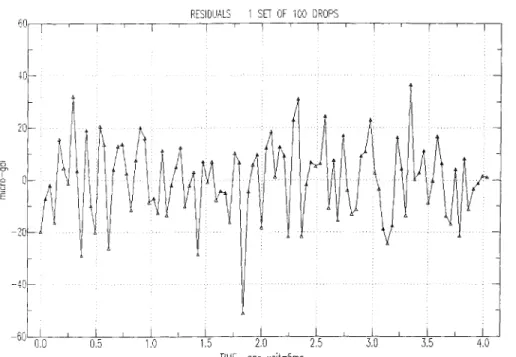
Figure 1. Dispersion of absolute gravity measurements during one set of 100 drops. The time interval between two drops is about 12.2 s and each set of 100 drops lasts about 20 min. The ordinate axis gives the gravity variations in ygal relative to a mean value. The standard deviation
on a single observation is 14.9 pgal, meaning that the standard deviation on the mean is then 1.5 pgal.
by guest on August 8, 2013
http://gji.oxfordjournals.org/
Calibration of a superconducting gravimeter 493
x - ? 1 l I I l I I I l I I I I I I I I I I I I l l I I I I I I I / I , I
196051 196101 146151 136201 13F251 196301 196351 1 TlllE UHIT=Smn
Figure 2. Absolute gravity measurements used in the experiment. The plotted values are the absolute gravity observations with the blue laser frequency (upper graph) and with the red laser frequency (lower graph). For easier viewing, an arbitrary offset has been added between the two graphs. We see that they essentially follow the tides. The time unit is 5 min and the gravity unit is 10'pgal.
of the pillar where the gravimeter is located. The temperature of the gravimeter room, which is inside an old fort built 100 years ago, is regulated to within 1°C. There are no roads or train tracks in the vicinity of the building situated in the field about 10 km away from Strasbourg.
The 'gravity' output (feedback voltage) is filtered by an antialiasing low-pass analogue filter before digitization every 2 s by a 5.5 digit analogue to digital converter. We use then a numerical low-pass symmetric filter to obtain gravity values every 5 min, which are stored by the data acquisition system. The resolution of the superconducting gravimeter is very high, at least better than 1 ngal; the often larger gravity residual noise (of a few ngal) observed with precise gravimeters is essentially dominated by meteorological effects (e.g. Wenzel & Zurn 1990).
2.3 The measurements
The series of absolute measurements consists of 5600 drops (56 sets of 100 drops) made on 1989 May 18 and May 19, over a period of 29hr in a room adjacent to the superconducting gravimeter. The microseismic noise level was low. During the experiment the room temperature rose from 21.3" to 21.7 "C. The drop-to-drop scatter was between 15 and 26pgal except for one set during a minor seismic event, where it was 40 pgal. A typical set is shown in Fig. 1.
The original purpose of the experiment was not to compare the superconducting and the absolute gravimeter on the tidal curve, but to determine the absolute value of gravity for future checks of the drift of the superconducting gravimeter. The last 51 sets were made by alternating red and blue laser frequencies; in additition, there are five sets in the beginning of the experiment made with the red frequency only, as shown on Fig. 2, which were kept in order to get a sufficient number of absolute observations at
the minimum of the tidal curve. The observations were screened plotting the empirical cumulative distribution set by set (Daniel & Wood 1980). Altogether eight outliers were identified and removed. From the superconducting gravimeter, filtered readings were available at 5 min intervals and a spline interpolation was used to provide data at the exact observation times of the absolute gravimeter.
3 RESULTS
The absolute and superconducting observations were compared on a drop-to-drop basis. Now, no matter how recent the laser calibration, at the pgal level we cannot assume that the separation between the red and the blue frequencies is known. Therefore, we must introduce two different offsets between the absolute and superconducting observations, one for each laser frequency. The model is then
ai, = Mil
+
p 1
+
E i l , ai, = mi,+
p2
+
Ei,, (1)where a, are the observations of the absolute gravimeter (in pgal), ri the output voltages from the superconducting gravimeter (in Volts); the subscript 1 refers to absolute measurements using the blue frequency, the subscript 2 using the red frequency. (Y is the calibration factor of the
superconducting gravimeter (in pgalV-'),
PI,
8,
are the offset values (in pgal) for each laser frequency, and ei (in pgal) are the errors of the absolute observations. The individual drop-to-drop errors of the absolute observations are much larger than the errors of the superconducting gravimeter readings, and these last ones will not be taken into account here. The linear phase shifi (-0.156"/cycle per day) introduced by the tide low-pass analogue filtering into the superconducting readings was taken into account.We have fitted model (1) using both the usual L, norm
by guest on August 8, 2013
http://gji.oxfordjournals.org/
494
J .Hinderer
et al.Table 1. Results for the simultaneous adjustment (see equation 1) between relative and absolute read- ings. The calibration factor (Y (in pgalV-') is sup-
posed to be unique whatever the laser frequency and
PI,
p2
are offset values (in pgal) (the subscript 1 is relative to absolute measurements using the blue laser, the subscript 2 using the red laser). The uncertainties for the L, estimates are 2a error bars (95 per cent confidence level).0 :3, $2
I,, i i o r i i i ~ 'iti.2S
*
0.4ti - 3.3s 0.64 - 1.71 k 0.58 L , Ii01'11l - 76.05 :3.19 1 .l'(least squares) and the L , norm (least absolute deviations). The L, norm is easy to implement numerically and analytical solutions exist for the uncertainties. The L, norm is known to give robust estimates because it minimizes the effect of outliers and of non-symmetric error distributions. However, it is more delicate to handle numerically and there is no direct estimate of the uncertainties.
The results are listed in Table 1. The residual standard error is 20.1 pgal for a single drop; in a similar kind of experiment made in Hannover, Wenzel (1988) found a value close to 70pgal. Note that all error bars given in this study are 2a, not l a ; they correspond hence to roughly 95 per cent confidence intervals. We skip the results for the offsets, since they are not of interest here. The uncertainties for the L, estimates were obtained by multiplying the uncertainties of the L, estimates by m ( 1 . 2 5 ) , which is asymptotically correct (Bassett & Koenker 1978).
The difference between L, and L, estimates is small. We prefer the L , estimate with the following motivation: the total squared error of an estimate consists of its variance and squared bias. For a Gaussian distribution, the L, has minimum variance (maximum precision). But because of the large number of drops the variance in our problem will be low for almost any estimator. Thus we are prepared to trade off some of this precision and use the L, estimate which is maximally resistant to bias (Clearbout & Muir 1973). Our preferred value for the calibration factor is then from Table 1:
( Y = -76.05*0.55pgalV-'.
The relative precision (at the 95 per cent confidence level) is better than 1 per cent (0.72 per cent). It must be noted that this is only a formal error related to the numerical adjustment and cannot therefore include systematic effects (especially if they are correlated with the tides).
4 SENSITIVITY A N A L Y S I S
Although the calibration was essentially performed over one tidal cycle only, the formal precision obtained for the calibration factor is surprisingly high, better than 1 per cent at the 95 per cent confidence level. However, due to eventual unaccounted systematic effects, it might very well be biased. In order to get an idea of the possible influence of these effects, we do here some supplementary analyses.
A natural way to proceed is to analyse separately the 'blue' and 'red' data sets. The model is then
ail = cu,ri1
+
b1
+
c i l , ai2 = aZri2+
82
+
~ i 2 , (3)where a, and ( Y ~ are now the calibration factors relative to
the absolute observations with the blue and red frequencies, respectively, and all other variables are as in equation (1).
We do not assume that the true ( Y ~ and a, factors differ; the
purpose of the model is diagnostic. We only quote here the results for least squares (the L, results do not differ much): a1 = -73.39
*
0.75 pgal V-',CU, = -77.03 f 0.68 pgal V-'. (4) The two solutions differ by about 2 per cent. The combined solution for (Y using L, norm (see Table 1) corresponds to
their weighted average, with the red getting somewhat larger weight. The difference between the two solutions demonstrates the importance of using both laser fre- quencies. If they drift in opposite directions, the effect is reduced in the mean. In this respect, the red/blue non-symmetry in the data gives rise to concern, but the results for the red frequency are not essentially changed when discarding the extra data from the beginning. However, assume that one frequency is stable and the other is drifting, not an uncommon situation. Then the bias in the joint solution is approximately 1 per cent. We therefore include in the model (1) two new parameters to account for a possible linear drift in the difference of absolute and superconducting observations, one parameter for absolute observations with each laser frequency. The model becomes
a,, = m,, + P I + Y l t l l + E l l , at2 = m.2 +
8 2
+ Y 2 f r 2+
E,2, ( 5 ) where y 1 and y , (in pgal per time unit) are drift coefficients for the blue and red observations respectively, and t, the observation times. We found(Y = -77.14
*
0.52 pgal V-',y , = 5.8 f 2.1 pgal day-', (6)
y2 = 3.1 f 1.4 pgal day-'.
The drift parameters are statistically significant. Drift could be caused by rising temperature for example (0.4 "C during the experiment) affecting the laser. However, Niebauer et al. (1988) found that for a similar laser, the temperature effect on the centre frequency was only 0.6 x "C-' or less than 0.3 pgal for the temperature change of 0.4 "C. The introduction of drift parameters changes the calibration factor by about 1 per cent with respect to the value from model (1) (see Table 1). Because of the non-symmetry in the tidal curve over the observation period, especially for the blue observations (Fig. 2), scaling the superconducting observations changes the separation absolute-super- conducting much like a linear drift does, i.e. the two types of parameters are correlated because of the design of the experiment (or lack of it). Longer parallel registrations over several tidal cycles are needed to separate systematic effects and to push down their influence on the result.
For our experiment, this influence can be estimated by comparing results from different models and data sets. For this purpose, we applied the model (5) with drift separately to the 'blue' and 'red' data sets and found calibration factors -76.6 pgal V-' and -77.4 pgal V-', respectively. The solutions thus range from -75.4 pgal V-' ('blue' data, no
drift model) to -77.4pgal V-' ('red' data with drift model),
by guest on August 8, 2013
http://gji.oxfordjournals.org/
Calibration of a superconducting gravimeter 495
which leads to a maximum difference of 1.5 per cent with respect to the solution from the preferred model (1) (cf. Table 1). We conclude that, in addition to the statistical uncertainty of less than 0.8 per cent (on the 2 a level), the calibration factor may contain a bias (systematic error) of up to 1.5 per cent because of the short time span and unfavourable design of the experiment. Assuming in the standard way that the unknown systematic error has a uniform distribution on the previous interval (-1.5, +1.5)
+
bias) is then2a level.
5 D I S C U S S I O N
In order to test the validity of the calibration factor, we performed a standard tidal least squares analysis using a set of 1.5yr (from 1988 January 1 to 1989 May 31) data recorded with the SCG 'IT70 in Strasbourg. The gravimeter feedback output voltages were converted in pgal using the calibration factor given by equation (2), corrected for local air pressure changes and the long-period part (zonal tides, instrumental drift, polar motion, long-period anomalies) was removed. As usually done when comparing observations with models (see e.g. Baker, Edge & Jeffries 1989), we choose here the diurnal 0, tidal wave as a reference wave for several reasons: its amplitude is large (more than 30 pgal in Strasbourg), the ocean load is quite well known and the atmospheric influence is weak. We get for the observed gravimetric factor 6 and phase K relative to this wave:
6,(0,) = 1.1488 f 0.0007,
~ ~ ( 0 ~ ) = 0.05" f 0.04", (7)
using 2 a error bars. It is noticeable that the value of 6 ( 0 , )
observed some years ago by Lecolazet at the same station using a Lacoste Romberg spring meter equipped with electrostatic feedback is 1.1474 (Souriau 1979; Melchior, Kuo & Ducarme 1976). The close agreement between these two values obtained with instruments calibrated by different methods is important because it provides an independent check, which is not the case when comparing a calibrated value to any theoretical model.
The observed gravity change
A,
can be written asTable 2. Ocean load computations for the tidal wave 0, in Strasbourg. Models (a) and (a') are with water mass imbalance accounted for, mod- els (b) and (b') without. All load computations shown here are based on the Schwiderski global ocean model, except models (a') and (b') where the North Atlantic contribution is computed using the Flather model.
b'ritricis (a) F r m & ( b ) Schrrneck ( a ) Schcrncck ( b ) Schorncck (a') Scherneck ( b ' ) Ducarme ( a ) Memi (a) M I ~ a r l ( b ) amplitude (pgal) 0.148 0.159 0.144 0.156 0.152 0.158 0.144 0.147 0.005 0.1ns f 0.002 ptiasrx ( d q p ~ ) l i l . 2 186.4 171.3 188.0 166.0 181.7 170.8 169.9 j,3.9 185.4 f i3.7
(Melchior 1983; see also Hinderer & Legros 1989):
-
A, = 6 , exp (~K,)A,
where A, is the gravity change that would be observed on a rigid Earth (the tilde denotes complex quantities). Before comparing the observations with a theoretical model for the body tide, one has to correct for :he ocean loading that we denote by
a,.
The corrected gravity change then becomesa,
=A,
-a,
= 6, exp (kC)Ar. (9) In Table 2 are listed different ocean load computations for our station. We see that the amplitude of the load is about 0.5 per cent of the body tide. There is a fair agreement (relative discrepancies of the order of a few per cent) in the amplitudes of the load and some larger uncertainties in the phase determination. When using the ocean load model (a'), which is the modified Schwiderski (1980) global model everywhere (with mass imbalance accounted for) except for the North Atlantic replaced by the Bidston model (Flather 1976), we get from equation (9):6,(0,) = 1.1536, ~ ~ ( 0 ~ ) = 0.01'. (10) Similarly, starting from model (a) (modified Schwiderski everywhere, with mass imbalance accounted for), we have
6,(0,) = 1.1534, ~ ~ ( 0 ~ ) = 0.03".
The main influence of the ocean load for the wave 0, is to increase the gravimetric factor (6,
>
6,) and to decrease the gravimetric phase (K,<
K , ) . An error estimate taking into account for this wave the small ocean loading contribution with respect to the body tide (A,/A,<<
1) and the fact thatK, and K, are small angles, shows that (to the dominant
order of approximation):
A(A, COS K I )
Ad, = Ah,
+
, AK,=AK,+ A(A, sin K , )Ar Ar6, '
(12) The uncertainty in the corrected gravimetric factor results from the error estimate on the observed value [which is essentially the one due to the calibration in addition to the (small) formal error coming from the tidal least-squares fit] and from the uncertainty in the real part of the ocean load
A, cos K, divided by A,. From Table 2, we can set an upper bound of 10 per cent relative error for this term. The induced error on 6, is then as low as (0.1)(0.5 X lop2) =
5 x For the corrected phase, the uncertainty in the imaginary part of the ocean load A , s i n ~ , (once again divided by A,) comes in addition to the error estimate on
the observed gravimetric phase K, (due to the tidal
least-squares fit). The discrepancies in the imaginary part are larger than the ones relative to the real part and we will assume here an upper bound of 40 per cent relative error (see also Neuberg et al. 1987). The induced error on K, is then about 0.025". Therefore, except if there are large errors in the ocean load computations, which are unlikely for 0, in Europe, the error on 6, is clearly dominated via 6 , by the uncertainty in the calibration factor. However, the error on
the corrected phase is dependent on the knowledge of the ocean load, a 40 per cent error in the imaginary part of the ocean load causing an uncertainty on K, as important as the observed value itself.
by guest on August 8, 2013
http://gji.oxfordjournals.org/
496 J. Hinderer et al.
0.08
-
0.06 -0.04 -
0 . 0 2
-
Let us compare the observed gravimetric factor corrected for ocean load with the theoretical value deduced from the Dehant-Wahr model, which is relative to the rotating, elliptical and elastic Earth. From table I11 in Dehant &
Ducarme (1987), the theoretical expression for 6 in our station (colatitude 0 = 41.5718") becomes
Q
0 . 0 0 1 4 d ( 7 cos2 8 - 3)
6 t h = 1.1551
-
= 1.1543.The model used in equation (13) for the elastic layered Earth is the 1066A model of Gilbert & Dziewonski (1975). There are however slight differences when using other Earth models like the PREM one (V. Dehant, personal communication, 1990). It can be shown that the changes due to inelasticity causes an increase in the gravimetric factor less than 0.1 per cent and negligible phase lags in the diurnal tidal band (Dehant & Zschau 1989).
Comparing (13) with (10) and (11) shows that the agreement between observation and theory is better than 0.1 per cent [-6.1 x lop4 for model (a') and -7.8 x lop4
for model (a) in relative values], the observed value (using the calibration factor (Y discussed in Section 3) being slightly
smaller than 6 t h . A comparison with
M 2
wave has shown a similar fair agreement and is not reported here. However,Gravimetric factor fcl Q (thl 1.13
'
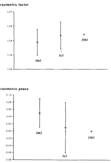
Grauimetric phase 0.10,Figure 3. Comparison between measured (m), ocean load corrected (c) and theoretical (th) values of the gravimetric factor and phase (in degrees) for the tidal wave 0,; the error bars are given at the 95 per cent confidence level.
even if observation and theory for the tidal gravimetric factor and phase are very close, the important point is to take into account the error bars. Considering the different error sources [tidal fit, ocean load (10 per cent error in real part and 40 per cent error in imaginary part), calibration precision], we would have a total uncertainty of 0.95 x lop2 on the corrected gravimetric factor and 0.07" on the phase for model (a') [the values using model (a) are similar]. Fig. 3 summarizes for the tidal wave 0, the relative locations of the observed, corrected and theoretical gravimetric factors and phases, with their (formal) uncertainties. We can finally conclude that the maximum discrepancy between 6, (only formal errors included) and St, reaches about 0.90 per cent (in relative values); the maximum lag between K , and irth (supposed to be zero) is less than 0.1" for both models.
6 CONCLUSIONS
Despite the limited time span (only one day), the comparison between absolute and relative gravity observa- tions performed in this study was shown to be able to provide a calibration factor with a precision of about 0.72 per cent at the 95 per cent confidence level. There is an excellent agreement (better than 0.1 per cent) between the gravimetric factor for the reference wave O , , which is observed with the superconducting gravimeter using this calibration constant and corrected for ocean loading, and the theoretical value relative to an elastic, rotating, elliptical, stratified Earth model. The uncertainty in the corrected gravimetric factor 6, is dominated by the uncertainty in the calibration (the error coming from the ocean load is weak) and is less than 1 per cent if the calibration uncertainty is represented by the precision quoted above. However, systematic effects connected with the short time span of our experiment (we are calibrating over one tidal cycle only), may in addition bias our result by about 1.5 per cent. Comparisons over larger time intervals (several tidal cycles at least) should improve the modelling of these effects and provide a more accurate calibration factor.
ACKNOWLEDGMENTS
We thank W. Ziirn for helping us in the tidal computation and for his useful comments on the manuscript. H. G. Scherneck, B. Ducarme and 0. Francis kindly provided their ocean load computations for our station. This study has been supported by CNRS-INSU DBT (Dynamique Globale) and is contribution number 314.
REFERENCES
Baker, T. F., Edge, R. J . & Jeffries, G., 1989. European tidal gravity: an improved agreement between observations and models, Geophys. Res. Lett., 16, 1109-1 112.
Bassett, G. & Koenker, R., 1978. Asymptotic theory of least absolute error regression, J . Am. Sfaf. Assoc., 73, 618-621. Claerbout, J. F. & Muir, F., 1973. Robust modelling with erratic
data, Geophysics, 38, 826-844.
Daniel, C. & Wood, F. S., 1980. Fitting Equations to Data, 2nd edn, Wiley, New York.
Dehant, V. & Ducarme, B., 1987. Comparison between the theoretical and observed tidal gravimetric factors, Phys. Earth planet. Inter., 49, 192-212.
by guest on August 8, 2013
http://gji.oxfordjournals.org/
Calibration
of
a superconducting gravimeter497
Dehant, V. & Zschau, J., 1989. 'The effect of mantle inelasticity ontidal gravity: a comparison between the spherical and the elliptical Earth model, Geophys. J . , 97, 549-555.
Faller, J. E., Guo, Y. G., Gschwind, J., Niebauer, T. M., Rinker,
R. L. & Xue, J., 1983. The JILA portable, absolute gravity apparatus, BGI Bull. Inf.. 53, 87-97.
Flather, R. A., 1976. A tidal model of the north-west European continental shelf, Mem. SOC. R. Sci. Liege, 10, 141-164. Gilbert, F. & Dziewonski, A. M., 1975. An application of normal
mode theory to the retrieval of structure parameters and source mechanisms for seismic spectra, Phil. Trans. R. SOC. Lond., A,
Hinderer, J. & Legros, H., 1989. Elasto-gravitational deformation, relative gravity changes and earth dynamics, Geophys. J . , 97, Lambert, A., Liard, J. O., Courtier, N., Goodacre, A. K.,
McConnell, R. K. & Faller, J. E., 1989. Canadian absolute gravity program. Applications in geodesy and geodynamics, EOS, Trans. Am. geophys. Un., 70, 1447-1460.
Melchior, P., 1983. The Tides of the Planet Earth, 2nd edn, Pergamon Press, Oxford.
Melchior, P., Kuo, J. T. & Ducarme, B., 1976. Earth tide gravity maps for Western Europe, Phys. Earth planet Inter., 13, Neuberg, J., Hinderer, J. & Ziirn, W., 1987. Stacking gravity tide observations in Central Europe for the retrieval of the complex eigenfrequency of the nearly diurnal free wobble, Geophys. J .
R. astr. Soc., 91, 853-868.
Niebauer, T. M., 1987. New absolute gravity instruments for physics and geophysics, PhD thesis, University of Colorado, Boulder, CO.
Niebauer, T. M., Hoskins, J. K. & Faller, J. E., 1986. Absolute gravity: a reconnaissance tool for studying vertical crustal 278, 187-269.
481-495.
184- 196.
motion, 1. geophys. Res., 91, 9145-9149.
Niebauer, T. M., Faller, J. E., Godwin, H. M., Hall, J. L. & Barger, R. L., 1988. Frequency stability measurements on polarization-stabilized He-Ne lasers, Appl. Optics, 27,
Peter, G., Moose, R. E., Wessells, C. W., Faller, J. E. & Niebauer, T. M., 1989. High-precision gravity observations in the United States, J. geophys. Res., 94, 5659-5674.
Schwiderski, E. W., 1980. Ocean tides, part I: global ocean tidal equations; Part 11; a hydrodynamical interpolation model, Mar. Geod., 3, 161-255.
Souriau, M., 1979. Spatial analysis of tilt and gravity observations of Earth tides in western Europe, Geophys. 1. R. astr. SOC., 57, Torge, W., Roder, R. H., Schniill, M., Wenzel, H.-G. & Faller, J. E., 1987. First results with the transportable absolute gravity meter JILAG-3, Bull. Geod., 61, 161-176.
Van Ruymbecke, M., 1989. A calibration system for gravimeters using a sinusoidal acceleration resulting from a vertical periodic movement, Bull. Geod., 63, 223-235.
Wenzel, H. G., 1988. Results of a test experiment to record tides with an absolute gravimeter, Proc. 66th JLG Meeting, pp. 13-14, ed. Poitevin, C.
Wenzel, H. G. & Ziirn, W., 1990. Errors of the Cartwright- Taylor-Edden 1973 tidal potential displayed by gravimetric Earth tide observations at BFO Schiltach, Bull. Inf. Markes Terrestres, 107, 7559-7574.
Wenzel, H. G., Ziirn, W. & Baker, T. F., 1990. In situ calibration of Lacoste-Romberg Earth tide gravity meter ET19 at BFO Schiltach, Bull. Inf. MarPes Terrestres, 109, 7849-7863. Zumberge, M. A., Rinker, R. I,. & Faller, J. E., 1982. A portable
apparatus for absolute measurements of the Earth's gravity, Metrologia, 18, 145-152. 1285-1289. 585-608. by guest on August 8, 2013 http://gji.oxfordjournals.org/ Downloaded from