Effects of Climate-induced Changes in Isoprene Emissions after the eruption of Mount Pinatubo

(1)

HAL Id: hal-03203403

https://hal.archives-ouvertes.fr/hal-03203403

Submitted on 21 Apr 2021

HAL is a multi-disciplinary open access

archive for the deposit and dissemination of

sci-entific research documents, whether they are

pub-lished or not. The documents may come from

teaching and research institutions in France or

abroad, or from public or private research centers.

L’archive ouverte pluridisciplinaire HAL, est

destinée au dépôt et à la diffusion de documents

scientifiques de niveau recherche, publiés ou non,

émanant des établissements d’enseignement et de

recherche français ou étrangers, des laboratoires

publics ou privés.

Distributed under a Creative Commons Attribution| 4.0 International License

Effects of Climate-induced Changes in Isoprene

Emissions after the eruption of Mount Pinatubo

P.J. Telford, J. Lathière, N.L. Abraham, A.T. Archibald, P. Braesicke, C.E.

Johnson, O. Morgenstern, F.M. O’connor, R.C. Pike, O. Wild, et al.

To cite this version:

P.J. Telford, J. Lathière, N.L. Abraham, A.T. Archibald, P. Braesicke, et al.. Effects of

Climate-induced Changes in Isoprene Emissions after the eruption of Mount Pinatubo. Procedia Environmental

Sciences, Elsevier, 2011, 6, pp.199-205. �10.1016/j.proenv.2011.05.021�. �hal-03203403�

(2)

Procedia Environmental Sciences 6 (2011) 199–205

Earth System Science 2010: Global Change, Climate and People

Effects of Climate-induced Changes in Isoprene Emissions

after the eruption of Mount Pinatubo

P.J. Telford

a*

, J. Lathière

b,c,d

, N.L. Abraham

a

, A.T. Archibald

a

, P. Braesicke

a

,

C.E. Johnson

e

, O. Morgenstern

a,f

, F.M. O’ Connor

e

, R.C. Pike

g

, O. Wild

c

,

P.J. Young

g,h

, D.J. Beerling

b

, C.N. Hewitt

c

and J.A. Pyle

a

a_{NCAS Climate, Centre for Atmospheric Science, Department of Chemistry, University of Cambridge, Cambridge, CB2 1NE, UK.} b_{Department of Plant and Animal Sciences, University of Sheffield. Sheffield, UK.}

c_{Lancaster Environment Centre, Lancaster University, Lancaster, LA1 4YQ, UK.} d_{now at Laboratoire des Sciences du Climat et de l'Environment, Gif sur Yvette France}

e_{Met Office Hadley Centre, Exeter, UK}

f _{now at National Institute of Water and Atmospheric Research, Lauder, New Zealand}

g_{Centre for Atmospheric Science, Department of Chemistry, University of Cambridge, Cambridge, CB2 1NE, UK} h_{now at NOAA Earth System Research Laboratory, Boulder, Colorado 80305, USA.}

.

Abstract

The eruption of Mt. Pinatubo in June 1991 was the largest in the twentieth century. One of its effects was to produce cooler and drier conditions in the years following the eruption. We present the results of an integrated model study of the effect of these climatic changes on the emissions of isoprene from the biosphere. Our emissions model simulations showed that global isoprene emissions were reduced by 9% from 1990 to 1992. When incorporated into our model of global atmospheric chemistry this reduction of isoprene emissions led to an increase in the tropospheric OH burden of 2%. This caused an increase in the removal of methane via oxidation by OH of up to 5 Tg per year. This could have contributed to the observed changes in methane growth rate at this time.

Selection under responsibility of S. Cornell, C. Downy and S. Colston.

Keywords: Pinatubo; isoprene; biogenic emissions; oxidising capacity; methane

* Corresponding author. Tel.: +44 (0)1223 336300; fax: +44 (0)1223 763823.

E-mail address: [email protected]

Open access under CC BY-NC-ND license.

(3)

200 P.J. Telford et al. / Procedia Environmental Sciences 6 (2011) 199–205

1. Introduction

The eruption of Mt. Pinatubo, on the island of Luzon in the Philippines in June 1991, was the largest in the twentieth century, injecting 20 Tg of SO2 into the stratosphere, which was rapidly converted into

sulfate aerosol [1]. This aerosol quickly spread around the globe reflecting shortwave radiation out to space and producing cooler temperatures across the Earth's surface [1]. The reduced incoming shortwave radiation also affected the hydrological cycle, reducing global precipitation and causing widespread drought [2]. In addition there was a strong El Niño event in 1992 [3], which changed temperature and precipitation patterns, for instance producing warmer and drier conditions in the Amazon.

At this time, the early 1990s, the growth rates of greenhouse gases dropped significantly [4,5]. The effect was most dramatic for methane, for which changes in both sources and sinks have been proposed. These decreases have been linked to reductions in anthropogenic emissions following the collapse of the USSR [6,7]. However, other factors contribute to the observed changes, including changes in emissions from wetlands [8] and biomass burning [9]. There have also been changes to the dominant sink of methane, its reaction with the hydroxyl radical (OH), proposed. These relate to changes in meteorology [10,11], changes in emissions of NOx (NO and NO2) and CO [12] and changes in UV radiation, affecting

photolysis in the troposphere [13].

We present results of a study [14] that investigated the effect of changes of biogenic emissions of isoprene on OH concentrations, and the consequences of these changes for methane. Isoprene is a reactive organic compound produced in large amounts from the global biosphere, mainly from tropical forests. Recent estimates of emissions have been around 500 Tg(C) per annum [15], an amount of carbon comparable to that from methane emissions [16]. Isoprene is also highly reactive, with a lifetime in the boundary layer on the order of hours, where it reacts with OH, ozone and the nitrate radical. The large emissions and high reactivity allow isoprene to influence the tropospheric oxidising capacity [17]. Isoprene emissions are sensitive to changes in temperature, humidity, insolation and precipitation [18].

The presented study [14] used climate dependent isoprene emissions in simulations of the UKCA chemistry climate model. The model was constrained by meteorological analyses to obtain the observed changes in climate over the period studied. The effects of changes in emissions were quantified by comparing the base simulation to a simulation where the emissions were fixed to values from before the eruption.

2. Model Description

Two models were used in the study; a parameterised emissions model to simulate the isoprene emissions and a chemistry climate model to investigate the impact of the emissions changes on atmospheric composition. The emissions model calculated the emissions in two stages; first a vegetation map was generated using the SDGVM vegetation model [19,20] from a time series of monthly mean temperature, humidity and downward shortwave radiation. The input for this model was taken from an earlier simulation of this period in the UKCA chemistry climate model [21]. The vegetation maps were combined with the climate data by a biogenic emissions model [22], that followed the empirical parameterisations of the MEGAN model [15] to produce isoprene emissions as functions of space and time.

The chemistry climate model used was a nudged version [23] of the UKCA chemistry climate model [24,25]. The UKCA model is based upon the Met Office's Unified Model [26]. In this study we used a horizontal resolution of 3.75×2.5°, 60 vertical levels from the surface to 84 km and a dynamical time-step of 30 minutes. A time series of sea surface temperatures and sea ice coverage were prescribed from the HadISST data-set [27]. The model was constrained using the technique of nudging to ERA-40 re-analysis

(4)

data [28] over the period of interest. The nudging was applied from 3 to 45 km with a relaxation time scale of 6 hrs [23]. We use the tropospheric chemistry of UKCA, which is a medium sized scheme. It simulates the Ox, HOx and NOx chemical cycles and the oxidation of CO, ethane, propane, and isoprene

[25]. The Mainz isoprene mechanism (MIM) [29] was used to parameterise isoprene oxidation. Methane was fixed at 1.76 ppmv to reduce time to spin up the model. A more detailed description of the model set-up can be found in Telford et al. [14].

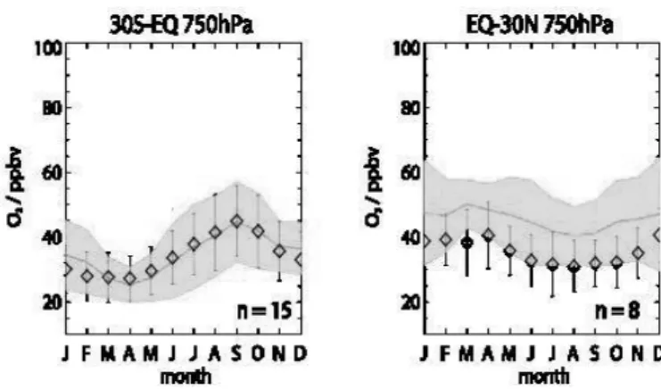
Figure 1 shows a comparison of modeled ozone with measured ozone from sondes in the lower tropical troposphere, using the approach of Stevenson et al. [30]. The comparison is restricted to the lower tropical troposphere, the region of the model where isoprene has the biggest impact. It can be seen that the model reproduces the ozone annual cycle of variability well here.

3. Results

In section 3.1 we discuss the changes in isoprene emissions caused by the climatic changes. In section 3.2 we present the effects of these changes on the oxidising capacity and methane. A more detailed analysis of the results is presented in Telford et al. [14].

3.1. Changes in Isoprene Emissions

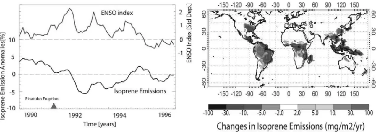
In this section we present an overview of the modelled changes in isoprene emissions during the early 1990s. The isoprene emissions anomalies over this period are shown in the left hand panel of Fig 2. The emissions start relatively high in 1990, before falling after the eruption to a minimum in 1992. After this the isoprene emissions rise to levels closer to those seen before the eruption. There were indications of a link between El Niño and the isoprene emissions, in agreement with the suggestions of Müller et al. [31] and Lathiére et al. [32], with the lowest values of the emissions occurring during La Niña conditions. However the correlation wasn't significant, possibly because it was obscured by the effects of the eruption.

To further understand the changes we examined their geographical distribution. The right hand panel in Fig. 2 maps the changes in isoprene emissions between 1992, the lowest values, and 1990, the highest. Decreases in emissions were simulated in most regions where isoprene was emitted. When we examine the drivers of isoprene emissions; temperature, humidity, radiation and precipitation, we find that these decreases were driven by the cooler and drier conditions found after the eruption. These reduce emissions in two ways. Firstly there was a direct reduction due to the parameterised decrease of the emissions with temperature. In addition there was a further, indirect, decrease relating to decreases in biomass caused by the cooler and drier conditions. The region where there was a notable increase was the Amazon basin, where localised warming caused by El Niño predominates over the global volcanic cooling.

Figure 1: Comparison of UKCA model ozone with sonde data in region of relevance for isoprene chemistry, the tropical lower troposphere.

(5)

3.2. Changes in Oxidising Capacity and Methane

We fed these isoprene emissions into the UKCA chemistry climate model, making three runs which are summarised in Table 1. The base run was the best guess for the period studied, including the effects of climate dependent isoprene emissions and variations in meteorology. To probe the effects of climate dependent isoprene emissions we used the EmFix run, identical to the Base run except that the isoprene emissions were fixed to 1990 values. In an analogous way we investigated the effect of changes in meteorology in the MetFix run by fixing the climate to 1990 conditions.

Table 1: Summary of runs made using UKCA.

Run Name Meteorology Emissions

Base 1990-1995 1990-1995

EmFix 1990-1995 1990

MetFix 1990 1990-1995

The effects of climate dependent isoprene emissions were obtained by taking the difference between the EmFix and Base runs. Similarly the effects of changes in meteorology were obtained by taking the difference between the MetFix and Base runs. The impacts on OH of changes in emissions and changes in meteorology evaluated in this way are shown in the left hand panel of Figure 3.

The decreased isoprene emissions increased tropospheric OH concentrations by up to 2%. The changes in meteorology decreased tropospheric OH by a similar amount, which in part relates to the cooler, drier conditions found after the eruption. The impact of the changing isoprene emissions was found to be comparable to the effects of changes in climate, indicating that changes in isoprene emissions can have a significant impact on tropospheric oxidising capacity. These changes in oxidising capacity were determined to have a notable effect on methane. As the methane concentration is fixed we could not examine these changes directly. Instead we calculated the flux through the reaction CH4+ OH for each

Figure 2: Changes in Isoprene Emissions in the 1990s. The left hand panel shows the anomalies in global isoprene emission anomalies through the early 1990s. The ENSO index of Wolter and Timlin [3] is included for reference. The right hand panel shows the distribution of changes between 1990 and 1992.

(6)

experiment to examine how the sink of methane changes. The changes in isoprene emissions led to an increase in the sink of methane of 5 Tg(C) per year, which is equivalent to a 1% reduction in methane

emissions. These changes are comparable to those estimated from biomass burning and wetland emissions [7]. We concluded that the climate dependent changes in biogenic emissions could contribute to the observed changes in methane concentrations at this time.

We plot the geographical distribution of the changes in tropospheric OH column caused by climate dependent isoprene emissions in the right hand panel of Figure 3. The local effect could be much larger than the global, up to 20% over eastern Africa, and was highly anti-correlated (-0.6) with the changes in isoprene emissions (see Fig 2).

4. Conclusion

Changes in climate caused by the eruption of Mt. Pinatubo and an El Niño warm event have been demonstrated to have a large impact on modeled isoprene emissions. These changes in emissions altered the concentration of OH, increasing the tropospheric column by up to 20% in regions such as eastern Africa and by 2% globally. The increased OH concentrations provided an increased sink for methane loss. This sink peaked at an extra 5 Tg of carbon per year, resulting to a variation in methane comparable to that from biomass burning and wetland emissions and equivalent to a 1% reduction in methane emissions. This demonstrates the importance of the whole Earth system in understanding changes in atmospheric composition and highlights the need to understand changes in the biosphere for future atmospheric and climatic changes.

Acknowledgements

This work was supported by NCAS and QUEST. We also acknowledge support through the EU FP6 Integrated Programme, SCOUT-O3(505390-GOCE-CT-2004). We acknowledge Paul Berrisford and the ECMWF for the ERA-40 data. The development of the UKCA model (www.ukca.ac.uk) was Figure 3: Changes in tropospheric oxidising capacity. The left hand panel shows the differences in tropospheric OH burden between the Metfix and Emfix and base runs, showing the effect of changes in isoprene emissions and meteorology. Six month running means are applied to show the long term trends. The right hand panel shows changes in tropospheric OH column between 1990 and 1992.

(7)

supported by the Joint DECC and Defra Integrated Climate Programme - DECC/Defra (GA01101) - and the Natural Environment Research Council (NERC) through the NCAS initiative.

References

[1] McCormick M, Thomason L, Trepte C. Atmospheric Effects of the Mount Pinatubo Eruption. Nature 1995; 373 (6513), 399– 405.

[2] Trenberth K, Dai A. Effects of Mount Pinatubo volcanic eruption on the hydrological cycle as an analog of geoengineering.

Geophys. Res. Lett. 2007; 34, 15,702.

[3] Wolter K, Timlin M. In: Proc. of the 17th Climate Diagnostics Workshop, Norman, OK, NOAA/N MC/CAC, NSSL, Oklahoma

Clim.Survey, CIMMS and the School of Meteor., Univ. of Oklahoma., 1993; pp. 52–57.

[4] Denman K, Brasseuer G, Chidthaisong A, Ciais P, Cox P, Dickinson R et al. Climate Change 2007: The Physical Science Basis.

Cambridge University Press 2007; pp. 499–587.

[5] Dlugokencky E, Houweling S, Bruhwiler L, Masarie K, Lang P, Miller J et al. Geophys. Res. Lett. 2003; 30, 1992.

[6] Wang J, Logan J, McElroy M, Duncan B, Megretskaia I, Yantosca R. A 3-D model analysis of the slowdown and interannual variability in the methane growth rate from 1988–1997. Glob. Biogeochem. Cyc., 2004; 18, GB3011.

[7] Bousquet P, Ciais P, Miller J, Dlugokencky E, Hauglustaine D, Prigent C, et al. Contribution of anthropogenic and natural sources to atmospheric methane variability. Nature 2006; 443, 439–443.

[8] Gedney N, Cox P, Huntingford C, Climate feedback from wetland methane emissions. Geophys. Res. Lett. 2004; 31, L20503. [9] Langenfelds R, Francey R, Pak B, Steele L, Lloyd J, Allison C. Interannual growth rate variations of atmospheric co2 and its

delta c-13, h-2, ch4, and co between 1992 and 1999 linked to biomass burning. Glob. Biogeochem. Cyc. 2002; 16, GB001466. [10] Johnson C, Stevenson D, Collins W, Derwent R. Interannual variability in methane growth rate simulated with a coupled

ocean-atmosphere-chemistry model. Geophys. Res. Lett. 2002; 29, 1903.

[11] Warwick N, Bekki S, Law K, Nisbet E, Pyle J. The impact of meteorology on the interannual growth rate of atmospheric methane. Geophys. Res. Lett. 2002; 29, 1947..

[12] Dalsøren S, Isaksen I. CTM study of changes in tropospheric hydroxyl distribution 1990-2001 and its impact on methane.

Geophys. Res. Lett. 2006; 33, L23811.

[13] Bekki S, Law K, Pyle J. Effect of ozone depletion on atmospheric CH4 and CO concentrations. Nature 1994; 371, 595–597.

[14] Telford P, Lathiére J, Abraham N, Archibald A, Braesicke, P, Johnson C, et al. Effects of climate-induced changes in isoprene emissions after the eruption of Mount Pinatubo. Atmos. Chem. Phys. 2010; 10, 7,117–7,125.

[15] Guenther A, Karl T, Harley P, Wiedinmyer C, Palmer P, Geron C. Estimates of global terrestrial isoprene emissions using MEGAN (Model of Emissions of Gases and Aerosols from Nature), Atmos. Chem. Phys. 2006; 6, 3,1813,210.

[16] Lelieveld J, Crutzen P, Dentener F. Changing concentration, lifetime and climate forcing of atmospheric methane. Tellus

Series B- Chem. & Phys. Met. 1998; 50 (2), 128–150.

[17] Zeng G, Pyle J. Changes in tropospheric ozone between 2000 and 2100 modeled in a chemistry-climate model. Geophys. Res.

Lett. 2003; 30, 1392

[18] Sharkey T, Wiberley A, Donohue A. Isoprene Emission from Plants: Why and How. Ann. Botany 2007; 10, 1–14. [19] Beerling, D, Woodward F, Lomas M, Jenkins A. Testing the responses of a dynamic global vegetation model to

environmental change: a comparison of observations and predictions. Glob. Ecology & Biogeog. Lett. 1997; 6, 439–50. [20] Beerling D, Woodward, F. Vegetation and the terrestial carbon cycle. Modelling the first 400 million years. Cambridge

University Press 2001.

[21] Telford P, Braesicke P, Morgenstern O, Pyle J. Reassessment of Causes of Ozone Column Variability following the Eruption of Mount Pinatubo using a nudged CCM, Atmos. Chem. Phys. 2009; 9, 4,251–4,260.

[22] Lathiére J, Hewitt C, Beerling, D. Sensitivity of isoprene emissions from the terrestrial biosphere to 20th century changes in atmospheric CO2 concentration, climate and land use. Glob. Biogeochem. Cyc. 2010; 24, GB1004.

[23] Telford P, Braesicke P, Morgenstern O, Pyle J. Technical note: Description and assessment of a nudged version of the new dynamics unified model. Atmos. Chem. Phys. 2008; 8, 1,701–1,712.

[24] Morgenstern O, Braesicke P, O’ Connor F, Bushell A, Johnson, C, Osprey, S, et al. Evaluation of the new ukca climate-composition model. part 1: The stratosphere. Geosci. Mod. Dev. 2009; 2, 43–57.

[25] O’ Connor F, Johnson C, Morgenstern, O, Sanderson, M, Young P, Collins W, et al. Evaluation of the new ukca climate-composition model. part 2: The troposphere. Geosci. Mod. Dev. Dis., in preparation

[26] Staniforth A, White A, Wood N, Thuburn J, Zerroukat M, Cordero E, et al. Joy of U.M. 6.1 - Model Formulation. United

Kingdom Meteorological Office (UKMO), 2005.

[27] Rayner A, Rayner N, Parker D, Horton E, Folland C, Alexander L, et al. Global analyses of sea surface temperature, sea ice, and night marine air temperature since the late nineteenth Century. J. Geophys. Res. 2003; 108D, 4,407.

(8)

[28] Uppala S, Kallberg P, Simmons A, Andrae U, Da Costa Bechtold V, Fiorino M, et al. The ERA-40 re-analysis. Q.J.R. Met.

Soc., 2005; 131, 2,961–3,012.

[29] Pöschl U, von Kuhlmann R, Poisson N, Crutzen P. Development and intercomparison of condensed isoprene oxidation mechanisms for global atmospheric modelling. J. Atmos. Chem. 2000; 37, 29–52.

[30] Stevenson D, Dentener F, Schultz M, Ellingsen K, van Noije T, Wild O, et al. Multimodel ensemble simulations of present-day and near-future tropospheric ozone. J. Geophys. Res. 2006; 111, D08301.

[31] Müller J, Stavrakou T, Wallens S, Smedt I, Roozendael M, Potosnak M, et al. Global isoprene emissions estimated using MEGAN, ECMWF analyses and a detailed canopy environment Model. Atmos. Chem. Phys. 2008; 8, 1,329–1,341. [32] Lathiére J, Hauglustaine D., Friend A, De Noblet-Ducoudré N, Viovy N, Folberth, G. Impact of climate variability and land