HAL Id: hal-00316771
https://hal.archives-ouvertes.fr/hal-00316771
Submitted on 1 Jan 2001
HAL is a multi-disciplinary open access
archive for the deposit and dissemination of
sci-entific research documents, whether they are
pub-lished or not. The documents may come from
teaching and research institutions in France or
abroad, or from public or private research centers.
L’archive ouverte pluridisciplinaire HAL, est
destinée au dépôt et à la diffusion de documents
scientifiques de niveau recherche, publiés ou non,
émanant des établissements d’enseignement et de
recherche français ou étrangers, des laboratoires
publics ou privés.
Observations of convection in the dayside
magnetosphere by the beam instrument on Geotail
H. Matsui, M. Nakamura, T. Mukai, K. Tsuruda, H. Hayakawa
To cite this version:
H. Matsui, M. Nakamura, T. Mukai, K. Tsuruda, H. Hayakawa. Observations of convection in the
day-side magnetosphere by the beam instrument on Geotail. Annales Geophysicae, European Geosciences
Union, 2001, 19 (3), pp.303-310. �hal-00316771�
Geophysicae
Observations of convection in the dayside magnetosphere by the
beam instrument on Geotail
H. Matsui1, M. Nakamura2, T. Mukai3, K. Tsuruda3, and H. Hayakawa3
1Space Science Center, Morse Hall, University of New Hampshire, Durham, NH 03824, USA
2Department of Earth and Planetary Science, University of Tokyo, Bunkyo-ku, Tokyo 113-0033, Japan 3Institute of Space and Astronautical Science, Sagamihara, Kanagawa 229-8510, Japan
Received: 24 August 2000 – Revised: 15 January 2001 – Accepted: 23 January 2001
Abstract. We report observations of magnetospheric
con-vection by the beam instrument, EFD-B, on Geotail. The region analyzed in this study is mainly the afternoon sector of the magnetosphere between L = 9.7 − 11.5. When the in-strument is operated, electron beams are emitted from guns and some of them return to detectors attached to the main body of the satellite. However, we find that the return beams are often spread over a wide range of satellite spin phase an-gles, so that the calculated convection is unreliable. In order to remove noisy data, we set up suitable selection criteria. We infer that the convection strength is of the order of 20 km/s. The convection has generally westward and outward com-ponents. This indicates that the plasma located at the satel-lite positions is being convected toward the magnetopause. Moreover, the obtained convection is highly variable because standard deviations are comparable to the strength. We then compare the convection estimated by the beam instrument with that by the particle instrument, LEP. We find that the convections derived from the two instruments are positively correlated, with correlation coefficients above 0.7. The anal-ysis reported here is expected to be useful in the interpreta-tion of the multi-spacecraft data from the Cluster II mission.
Key words. Magnetospheric physics (current systems;
elec-tric fields; instruments and techniques)
1 Introduction
A knowledge of magnetospheric convection is central in or-der to unor-derstand various magnetospheric processes. It is a quantity needed to study the transport of particles in the mag-netosphere, such as the outflow of the ionospheric plasma (e.g. Matsui et al., 1999). It is a basic input to studies of the energization and decay of the ring current (e.g. Jordanova et al., 1999). Study of the magnetospheric convection pat-terns would clarify the mechanisms of the response of the magnetosphere to momentum transfer from the solar wind.
Correspondence to: H. Matsui ([email protected])
For these reasons, a number of instruments working on dif-ferent physical principles have been devised. Examples of these instruments are: 1) the beam instrument, 2) the probe instrument, and 3) the particle instrument. We can determine convection by the beam instrument with high accuracy. The technique employed by the beam instrument measures di-rectly the drift motion of electrons. The electrons drift across the magnetic field, and in addition, gyrate around it, so that the orbit is primarily far away from the main body of the satellite. Compared to other methods, measurement of con-vection by the beam instrument is, thus, hardly at all affected by the cloud of photoelectrons in the vicinity of the satellite. Magnetospheric convection was derived from a beam in-strument for the first time by Baumjohann et al. (1985), who analyzed data obtained by GEOS 2 at geosynchronous or-bit. Baumjohann et al. (1985) confirmed that the convection strength depends on the level of geomagnetic activity. Re-cently, Quinn et al. (1999) reported convection obtained by the Equator-S satellite, also using the beam technique. The convection was found to have large AC components. This is also true for an example of convection obtained by Geotail (Matsui et al., 2000). In the Geotail study, convection was not difficult to determine because of the following reasons: 1) return beams are detected twice per spin period as they are scanned, according to the spin motion of the satellite. 2) the ranges of spin phases with return beams are narrow. 3) time variations of spin phases with return beams are small.
In this study, we analyze a sample of convection data from seven Geotail orbits using the beam technique. The quality of the data is not always as good as described above, so that we shall develop new criteria to obtain reliable convection values. We then calculate averages and standard deviations of the convection for each orbit and relate them to the geo-magnetic activity, as parameterized by the Kp index. As a check on the convection inferred from the beam instrument, we compare the results with those obtained by the particle in-strument. This exercise will help in the near future the studies of convection patterns obtained from beam instruments, such as Cluster II.
304 H. Matsui et al.: Convection in the dayside magnetosphere Gun Detector Detector Gun spin axis, magnetic field d d spin axis, magnetic field
a
b
Gun Detector Detector Gun spin axis, magnetic field d d spin axis, magnetic fielda
b
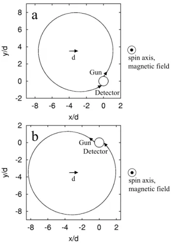
Fig. 1. Configuration of an electron gun and detector attached to the
main body of the satellite. The orbits of electron beams are depicted for a simple case when the magnetic field is parallel to the spin axis. In the example shown, B0=104nT and the drift step vector d = 2
m in the +Y direction for a cyclotron period. Return beams are detected for the two spin phases, as shown in a and b.
2 Instrumentation
In this study, we use data obtained by the beam instrument on Geotail. Details of the configuration of the instrument are given in Tsuruda et al. (1994, 1998). The beam instrument consists of electron guns and detectors, as shown in Fig. 1. Electron beams of energy 769 eV are released from the guns attached to the main body of the satellite in a direction ap-proximately perpendicular to the magnetic field, as obtained by the onboard magnetometer (Kokubun et al., 1994). The subsequent motion of the electrons is a combination of cy-clotron and drift motions (mostly the E × B drift motion). In general, the drift velocity is much slower than the velocity of the electron beams, so that some of the electrons return to the satellite after approximately one cyclotron period from the time when they were released from the gun. Such a con-dition generally happens twice per spin period, as indicated in the figure, where we show a specific case with B0 =104 nT and drift step vector d = 2 m in the +Y direction for a cyclotron period.
l
1
l
2
g
1
g
2
d
d
1
,d
2
Fig. 2
s
Fig. 2. Geometry for calculating magnetospheric convection. The
plane shown is perpendicular to the magnetic field. Electron beams are emitted from the locations g1and g2. After about one cyclotron
period, the beams are detected at the locations d1and d2. The loca-tions of the guns and detectors are moved in parallel so that d1and d2are superposed.
Typical ambient plasma conditions during the operational period of the instrument are as follows: magnetic field strength ∼80 nT, number density ∼1 cm−3, and electron temperature ∼1 keV. With these parameters, the cyclotron radius is 1.2 km, while the Debye length is 230 m. As antic-ipated earlier, our observations are not much affected by the cloud of photoelectrons around the satellite.
3 Data processing
In the analysis, we determine convection by using the drift step method (Melzner et al., 1978), rather than using the tri-angulation method (Paschmann et al., 1997). The convec-tion strength is determined in both methods by using the geometrical relation between guns and detectors. The lat-ter method is suitable for observations with guns capable of sweeping in the whole solid angle, whereas only elevation angles from the spin plane can be controlled for the Geotail observations, similar to the GEOS observations (Melzner et al., 1978). Elevation angles, at which electrons are released, are set as the angles approximately perpendicular to the am-bient magnetic field. Azimuthal angles are variable
depend-1999/03/13 2 4 log(counts) Top Bottom 0 0 90 90 180 180 270 270 360 360
Spin Phase (deg.)
Spin Phase (deg.)
0 50 |V| (km/s) -90 90 (deg.) θ -180 180 (deg.) φ UT 0500 0510 0520 0530 Fig. 3
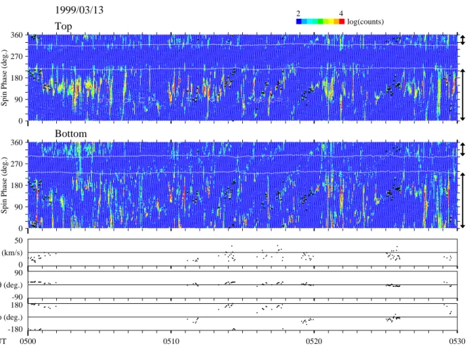
Fig. 3. Return beams measured by the detectors on 13 March 1999. The quantity of return beams is shown by a color contour for the top
and bottom detectors. The data are sorted by time and spin phase. The black marks in the upper two panels show the spin phases which are used to determine convection. Arrows on the right side of each panel show the approximate view angles possible for detecting beams. The white line shows limits of such spin phases. There are two lines during most of the time period, indicating that there is an interval where it is hard to detect return beams for each spin period. However, occasionally, there are four lines, indicating that there are two intervals where it is hard to detect return beams. The bottom three panels show the convection strength |V |, its elevation θ , and azimuthal angles φ.
ing on the spin motion of the satellite. We do not use the time-of-flight method (Tsuruda et al., 1994), in which the convection strength is determined by using the time-of-flight of electron beams between guns and detectors. This method would be unreliable in the region analyzed in our study, since the resolution is not very good. The time-of-flight method is more suitable in a region with a long gyration period, such as the magnetotail.
For time-stationary, uniform electric field, return beams are detected twice per spin period. An example of such con-figurations is shown in Fig. 1. In this example, the spin axis is chosen to be parallel to the magnetic field. However, this is not true, in general, so that the procedure to derive con-vection is more complicated. The geometry for such a case is shown in the plane perpendicular to the magnetic field in Fig. 2. Configurations for two spin phases for which there are return beams are moved in parallel, so that both detectors are superposed. Return beams are detected if the beams are pointing towards s, or away from s, where s is the source point of the drift step vector. Here, we assume the gun fir-ing direction and the direction of the detector are parallel
be-cause the cyclotron radius is much longer than the drift step length. When we derive the drift step vector, it is necessary to know the gun firing directions at the times when beams are returning, and the distance between the emitted and the detected beams. The magnitude of the drift velocity is larger when both gun firing directions are almost antiparallel, since l1 and l2 are close to being perpendicular to the drift step vector d. The magnitude is smaller when both of the firing directions are almost parallel. In that case, l1and l2are close to being parallel to d. We can determine the direction of convection because the direction of the electric field, which is perpendicular to that of the convection, lies between the two gun firing directions. The time resolution in the derived convection is the same as the spin period if there is only one gun-detector pair. In the Geotail instrument, there are two gun-detector pairs located at the top and bottom sides of the satellite. The gun-detector pairs have a spin phase shift of 180◦with respect to each other, so that the time resolution is half the spin period. One more point which should be noted about the characteristics of the instrument is that a part of the beams returning to the detector cannot be received because
306 H. Matsui et al.: Convection in the dayside magnetosphere the guns and detectors have finite view angles. Particles with
an elevation angle approximately between −30◦and 20◦are measured by the top detector, while those with an elevation angle approximately between −25◦and 35◦are measured by the bottom detector. Nevertheless, the angle between the spin axis and the magnetic field in the dayside equatorial magne-tosphere, which is the region examined in the study, is not large because the spin axis is close to the Z axis in the geo-centric solar ecliptic (GSE) coordinate system. In that case, electron beams tend to be received by the detectors.
The quality of the data for one orbit, analyzed by Matsui et al. (2000), is high, as mentioned in the introduction. How-ever, this is not always the case. Such an example occurred on 13 March 1999. The return beams for the top and bot-tom detectors are shown in the top two panels of Fig. 3. In this case, spin phases with return beams are variable, which presumably results from the existence of Pc 1 waves of fre-quency ∼0.7 Hz, as confirmed by wave spectra of the mag-netic field (Figure not shown). Return beams are sometimes observed over a wide angular range of spin phases. This is true, for example, for the beams observed by the top detector with spin phases around 150◦at 0503 UT. At other times, the return beams are confined to a narrow range of spin phases, so that we can determine convection. Such an example is obtained at 0519 UT.
Thus, it is necessary to pick out intervals during which we can obtain reliable convection. To this end, we set the fol-lowing five criteria. First, we only use average values of spin phases inside 10 degrees within the expected angular range for detecting return beams. Otherwise, the calculation of av-erages could be biased since a sizable fraction of beams can-not be detected. In Fig. 3, the spin phases within the approx-imate view angles possible for detecting beams are indicated by arrows at the right side of the top two panels. The white lines show the limits of such spin phases. Second, the next criterion is set as
|φt−φb| ≥5◦, (1)
where φt and φbare averages of spin phases of the top and bottom detectors with return beams, respectively. The crite-rion gives an upper limit to the convection strength. If the criterion is not satisfied, the error in estimating convection strength is larger since the drift step length is much longer than the distance between guns and detectors. In that case, the firing direction for one gun is close to anti-parallel to that for the other gun since the two guns are attached with a shift of a spin phase with 180◦to one another, as noted previously. When we obtain φt and φb, we collect spin phases with re-turn beams with counts above 200. The interval when the particles may be received is approximately 1/4 of the spin period. We then form averages of spin phases with return beams. Third, the next criterion is related to the divergence of return beams. We require that:
1φt ≤5◦, (2)
1φb≤5◦, (3)
where 1φtand 1φbare standard deviations of the spin phases with return beams around φt and φb, respectively. Fourth, if the shapes of the variations of spin phases with return beams at the top and bottom detectors are similar, we can make reli-able inference on the convection. Thus, we set one criterion related to the angular width of the beam:
0.5 < 1φt 1φb
<2. (4)
Finally, we calculate the correlation between φt and φb for data acquired over each one minute interval. The minimum number of data points to calculate a correlation is five. This selection criterion then requires that
r >0.98, (5)
0.8 < β < 1.25, (6)
where r is the correlation coefficient, and β is the slope of the regression line of φbto φt.
The spin phases which are finally selected to calculate con-vection are shown with black marks in Fig. 3. Although inter-vals with the black marks are much shorter than those with-out the marks, the patterns of the marks are similar at the top and bottom detectors.
4 Observations
4.1 Convection derived from the beam instrument
Convection on 13 March 1999 is shown in the bottom three panels in Fig. 3. We subtract the velocity of the satellite, so that each value is shown in an inertial frame. The eleva-tion and azimuthal angles of the conveceleva-tion are calculated in the solar magnetospheric (SM) coordinate system. The con-vection strength varies around 19 km/s. The elevation angle varies little about θ ∼ 0◦, while the azimuthal angle is either φ ∼ −30◦or φ ∼ 150◦.
We next examine the convection obtained by the beam in-strument for the seven orbits, as shown in Fig. 4. The orbits are located mainly in the afternoon sector of the magneto-sphere between 10.2−18.0 magnetic local time (MLT ). The Lvalue varies between 9.7−11.5. We select the MLT range because the electron number density from the plasma sheet is low. If the number density is large, magnetospheric electrons with an energy similar to that of the emitted beams could damage the detector.
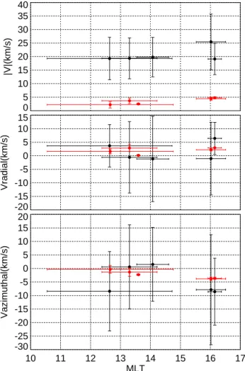
Black points and lines in Fig. 5 show averages and stan-dard deviations of the convection on five orbits within the seven orbits analyzed in this study. (We cannot determine convection at any time on 20 January 1999 and 20 February 1999, either because return beams are observed over a wide range of spin phases or because there are few return beams.) For these five orbits, averages of the convection strength are estimated to lie between 19 and 25 km/s. In the next panels, components with positive signs mean outward and eastward directions, respectively. The average azimuthal component lies between −9 and 2 km/s, as expected from the direction
-5
0
5
10
15
-5
0
5
10
15
XSM(Re)
YSM(Re)
Orbits with EFD-B Operation
930411 941121 990120 990125 990220 990308 990313
-10
-5
0
5
10
-5
0
5
10
15
ZSM(Re)
YSM(Re)
Orbits with EFD-B Operation
930411 941121 990120 990125 990220 990308 990313
Fig. 4
-5
0
5
10
15
-5
0
5
10
15
XSM(Re)
YSM(Re)
930411 941121 990120 990125 990220 990308 990313-10
-5
0
5
10
-5
0
5
10
15
ZSM(Re)
YSM(Re)
Orbits with EFD-B Operation
930411 941121 990120 990125 990220 990308 990313
Fig. 4
Fig. 4. Seven orbits on which the beam instrument is operated.Locations of the satellite are shown in the SM coordinate system. Dates are noted beside the locations of the orbits.
of convection outside the corotation region. Moreover, the radial component lies between −1 and 6 km/s, as expected for particles which are being convected outward toward the magnetopause. The direction of the observed convection is consistent with that derived by Baumjohann et al. (1985) at geosynchronous orbit from GEOS 2, under moderate geo-magnetic activity. However, the fluctuations are comparable to the convection strength. Such a result indicates that parti-cle orbits with AC components could be largely shifted from those estimated by a model incorporating only a DC
compo-0 5 10 15 20 25 30 35 40 |V|(km/s) -20 -15 -10 -5 0 5 10 15 Vradial(km/s) 10 11 12 13 14 15 16 17 MLT -30 -25 -20 -15 -10 -5 0 5 10 15 20 Vazimuthal(km/s)
Fig. 5
Fig. 5. Averages and standard deviations of observed and modeled
convection for five orbits analyzed in this study. Averages are shown by circles, while error bars denote standard deviations. Observed convection is shown with black color, while modeled convection is shown with red color. The horizontal axis shows the magnetic lo-cal time of measurements. Positive values in the second and third panels correspond to the outward and eastward convection, respec-tively.
nent.
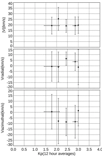
Another point which we are interested in is the dependence of convection on geomagnetic activity, parameterized by the Kpindex. Fig. 6 shows this dependence. Twelve hour aver-ages have been used. No clear features emerge. In the figure, the Kp values are in the range of 1.4 − 3.0 (low to moderate activity). If Kp values are larger, the satellite would possibly be located outside the magnetosphere (Matsui et al., 1999). There is one orbit on 20 January 1999 with Kp values less than one, but we are unable to determine the convection on this orbit.
4.2 Comparison with convection obtained by the particle instrument
When the beam instrument is operated, the particle instru-ment (Mukai et al., 1994) is operated as well. Since one
ma-308 H. Matsui et al.: Convection in the dayside magnetosphere 0 5 10 15 20 25 30 35 40 |V|(km/s) -20 -15 -10 -5 0 5 10 15 Vradial(km/s) 0.0 0.5 1.0 1.5 2.0 2.5 3.0 3.5 4.0 Kp(12 hour averages) -30 -25 -20 -15 -10 -5 0 5 10 15 20 Vazimuthal(km/s)
Fig. 6
Fig. 6. Averages and standard deviations of convection for five
or-bits analyzed in this study. Kp values averaged over an interval of 12 hours are shown in the horizontal axis.
jor aim of this paper is to obtain reliable convection from the beam instrument, it is useful to compare convections derived from the two instruments. Particle data are available on four orbits. Figure 7 shows a scatter plot of convections obtained by the two instruments on these orbits. We work in the satel-lite coordinate system which is close to the GSE coordinate system. Time resolution is different for each instrument, so that in Fig. 7, we compare 1-min average values. For the particle data, we subtract the component of the velocity vec-tor parallel to the magnetic field because the beam instrument only gives a velocity perpendicular to the magnetic field. The convection components estimated from the two instruments are positively correlated with correlation coefficients above 0.7. The regression lines in a unit of km/s are as follows: VX(particle) = 1.43 + 0.73VX(beam) (r =0.82), (7) VY(particle) = −12.75 + 0.92VY(beam) (r =0.84), (8) VZ(particle) = 7.56 + 0.93VZ(beam) (r =0.71). (9) It may be noted that there are offsets in the Y and Z compo-nents of the derived convection velocities, which we discuss below. -20 -10 0 10 20 30 40 50 -25 -20 -15 -10 -5 0 5 10 15 20 25 30 Vx(PARTICLE) km/s Vx(BEAM) km/s y=1.43+0.73*x r=0.82 -60 -50 -40 -30 -20 -10 0 10 -30 -25 -20 -15 -10 -5 0 5 10 15 20 25 Vy(PARTICLE) km/s Vy(BEAM) km/s y=-12.75+0.92*x r=0.84 -5 0 5 10 15 20 25 30 35 -15 -10 -5 0 5 10 Vz(PARTICLE) km/s Vz(BEAM) km/s
Fig. 7
y=7.56+0.93*x r=0.71 -20 -10 0 10 20 30 40 50 -25 -20 -15 -10 -5 0 5 10 15 20 25 30 Vx(PARTICLE) km/s Vx(BEAM) km/s y=1.43+0.73*x r=0.82 -60 -50 -40 -30 -20 -10 0 10 -30 -25 -20 -15 -10 -5 0 5 10 15 20 25 Vy(PARTICLE) km/s Vy(BEAM) km/s y=-12.75+0.92*x r=0.84 -5 0 5 10 15 20 25 30 35 -15 -10 -5 0 5 10 Vz(PARTICLE) km/s Vz(BEAM) km/sFig. 7
y=7.56+0.93*x r=0.71 -20 -10 0 10 20 30 40 50 -25 -20 -15 -10 -5 0 5 10 15 20 25 30 Vx(PARTICLE) km/s Vx(BEAM) km/s y=1.43+0.73*x r=0.82 -60 -50 -40 -30 -20 -10 0 10 -30 -25 -20 -15 -10 -5 0 5 10 15 20 25 Vy(PARTICLE) km/s Vy(BEAM) km/s y=-12.75+0.92*x r=0.84 -5 0 5 10 15 20 25 30 35 -15 -10 -5 0 5 10 Vz(PARTICLE) km/s Vz(BEAM) km/sFig. 7
y=7.56+0.93*x r=0.71Fig. 7. Correlation between convections obtained by the beam
in-strument and those by the particle inin-strument. The regression lines and the correlation coefficients are also shown in the figure.
5 Discussion
In this paper, we have examined convection data measured by the beam instrument on Geotail mainly in the afternoon sector of the magnetosphere. Here, we have a discussion rel-evant to the results obtained.
First, we compare the convection with that estimated, us-ing the model of Weimer (1995). Locations at which the
elec-tric potential was modeled by Weimer (1995) referred to the ionosphere at low-altitude. Thus, we map the potential distri-bution to Geotail locations by using the magnetic field model (Tsyganenko, 1989). We assume that the electric potential is constant along magnetic field lines. It is necessary to input interplanetary magnetic field data into the model of Weimer (1995), for which we use key parameters from IMP-8, Wind, and ACE at CDAWeb site. The calculated convection at the locations of Geotail is shown with red points and lines for each orbit in Fig. 5. The model convection speeds, which lie between 3.4 − 4.5 km/s, are much smaller than those from our observations of the order of 20 km/s. One reason for the discrepancy might be that the actual magnetic field sampled by Geotail is inclined from that in the model. If the mapped location is not appropriate, the estimated potential is differ-ent from the actual one. Another reason might be the exis-tence of a field-aligned potential close to the magnetopause. With regards to the direction of convection, the radial com-ponent estimated from the model is outward, which is also generally observed. The azimuthal component is westward in the model and the observations. However, the standard deviation of the convection estimated from the observations is much larger than that from the model, which indicates that the actual motion of the particles is variable to a large degree. In this study, the dependence of convection on the Kp in-dex over a restricted range is not clear. It is commonly known that convection depends on the level of geomagnetic activity (Baumjohann et al., 1985). Recently, Rowland and Wygant (1998) reported dependence of the electric field on the Kp index based on observations by the CRESS probe instrument made between L = 2.5 − 8.5, which is lower than the L value of the Geotail examples. Although the dependence is clear for L ≤ 6, it is less evident for larger L values with 16 − 21 MLT . As the L values of the Geotail locations are larger, the result by Rowland and Wygant (1998) is consis-tent with our result. However, the issue is important enough to merit further study with more extensive data sets (for ex-ample, Cluster II).
When we compare the convection from the beam instru-ment with that from the particle instruinstru-ment, each component is positively correlated with correlation coefficients above 0.7. This indicates that the results obtained by the beam in-strument are relatively reliable. However, we find offsets in the Y and Z components. One reason for the offsets is that the effect of drift other than the E × B drift is not negligible for the particle instrument, because the upper limit of the en-ergy range of this instrument is high (39 keV for ions). Such an effect results approximately from the current perpendicu-lar to the magnetic field, as shown in the following equation, where terms related to electron pressure and time variation of velocity of ions and electrons are neglected.
V (particle) − V (beam) ∼ 1
neJ⊥. (10)
Here, n is the number density, e is electronic charge, and J⊥ is current perpendicular to the magnetic field. Yoshimura and Iijima (manuscript in preparation, 2000) estimated the
perpendicular current in the −Y (dawnward) direction to be 1 − 2 nA/m2 in the dayside magnetosphere, based on the magnetic field data obtained by Geotail. If we assume a par-ticle density of 0.5 cm−3, the drift velocity is estimated as 13 − 25 km/s, which is close to the observed offset in the −Y direction (12.75 km/s). The effect of drift other than the E × B drift may also be expressed as the divergence of the ion pressure tensor ∇ · Pi.
V (particle) − V (beam) ∼ 1
neB2B × (∇ · Pi). (11) For the Geotail observations, the drift resulting from ∇Pi is estimated as a few km/s, where Pi is the scalar ion pressure (Matsui et al., 1999). Lui and Hamilton (1992) estimated the current resulting from ion pressure, taking into account anisotropy by using the data obtained by AMPTE CCE. Al-though the error bar is large, the perpendicular current ob-tained at apogee (L ∼ 8.8 RE) is less than 1 − 2 nA/m2. We can also estimate the offset by using the magnetic field model of Tsyganenko and the observed temperature with the following equation:
V (particle) − V (beam) ∼ Ti⊥
eB3B × ∇B + Tik
eB4B × [(B · ∇)B], (12) where Ti⊥ and Tik are the temperature of ions perpendicu-lar and parallel to the magnetic field, respectively. Here we include the effect of gradient drift and curvature drift. The offset is estimated as a few km/s, at most, so that it cannot explain the observed offset as large as 12.75 km/s. In that case, other effects could be important. One possible reason for the offset in the Z component of convection is the effect of drift other than the E × B drift, just as for the Y compo-nent. Another source for this offset may be the slightly differ-ent efficiency of detectors of the particle instrumdiffer-ent. There are seven particle detectors on Geotail (Mukai et al., 1994), each of which has a different viewing elevation angle.
We should be careful about drawing general conclusions when we take into account the following points: 1) The num-ber of orbits used in this study is small; 2) The Kp range for the orbits with available convection is restricted to low val-ues (1.4 − 3.0); 3) We do not analyze the data if the criteria given in Sect. 3 are not satisfied. When we apply these cri-teria, we could determine convection only about 2% of the time. It is left for future work to determine how to improve this number; 4) The electron guns and detectors have finite view angles, as previously discussed. In that case, the con-vection is hard to determine in some directions if there is an oblique angle between the spin axis and the magnetic field. Actually, this is true for cases when the azimuthal direction of convection is 70◦or 250◦from the sun; 5) We set an up-per limit to the convection strength. When we refer to Fig. 5, average values of convection are relatively similar, between 19 and 25 km/s, due to this upper limit.
In this study, we have analyzed data from the beam instru-ment on Geotail. Beam instruinstru-ments are also being flown on
310 H. Matsui et al.: Convection in the dayside magnetosphere the four spacecraft on the Cluster II mission, which has
re-cently started (Paschmann et al., 1997). It is useful to apply and to extend the above analysis with these data. The qual-ity of the Cluster II data will be better since there are many improved aspects in the hardware; for example, the detector covers the entire solid angle. The availability of data from four spacecrafts close to each other opens the possibility of cross correlating results. The present work is important to assess what pitfalls one might meet in that analysis and how to overcome them.
6 Conclusions
We have reported observations of convection in the dayside magnetosphere by the beam instrument on Geotail. When the instrument is operated, we try to detect beams emitted from the guns. However, return beams are often observed in a wide range of spin phases, so that we have developed crite-ria to obtain reliable convection. We have analyzed data for seven orbits, mainly in the afternoon sector of the magneto-sphere, close to the magnetopause. The convection strength is of the order of 20 km/s. The convection direction is gener-ally westward and outward, indicating that the plasma at the Geotail locations is convected toward the magnetopause. The derived convection has large standard deviations. When we compare convection obtained by the beam instrument with that obtained by the particle instrument, we obtain a positive correlation with correlation coefficients above 0.7. We also compare the convection with that from the model of Weimer (1995). The convection strength is larger in the actual ob-servations. However, one must bare in mind that the amount of data analyzed is relatively small. Recently, Cluster II has been launched so that data with higher quality will be soon available. We expect analysis reported here to be useful in the interpretation of these data.
Acknowledgements. J. M. Quinn and C. J. Farrugia gave us
use-ful comments to improve the manuscript. We would like to thank T. Nagai for providing the magnetic field data of Geotail. We are grateful to A. Szabo, R. Lepping, and N. Ness for use of the key parameter data of magnetic field of IMP-8, Wind, and ACE used in this study.
Topical Editor G. Chanteur thanks G. Paschmann and E. Whip-ple for their help in evaluating this paper.
References
Baumjohann, W., Haerendel, G., and Melzner, F., Magnetospheric convection observed between 0600 and 2100 LT: Variation with
Kp, J. Geophys. Res., 90, 393–398, 1985.
Jordanova, V. K., Farrugia, C. J., Quinn, J. M., Torbert, R. B., Borovsky, J. E., Sheldon, R. B., and Peterson, W. K., Simula-tion of off-equatorial ring current ion spectra measured by Polar for a moderate storm at solar minimum, J. Geophys. Res., 104, 429–436, 1999.
Kokubun, S., Yamamoto, T., Acu˜na, M. H., Hayashi, K., Shiokawa, K., and Kawano, H., The GEOTAIL magnetic field experiment, J. Geomag. Geoelectr., 46, 7–21, 1994.
Lui, A. T. Y. and Hamilton, D. C., Radial profiles of quiet time magnetospheric parameters, J. Geophys. Res., 97, 19325–19332, 1992.
Matsui, H., Mukai, T., Ohtani, S., Hayashi, K., Elphic, R. C., Thom-sen, M. F., and Matsumoto, H., Cold dense plasma in the outer magnetosphere, J. Geophys. Res., 104, 25077–25095, 1999. Matsui, H., Nakamura, M., Terasawa, T., Izaki, Y., Mukai, T.,
Tsu-ruda, K., Hayakawa, H., and Matsumoto, H., Outflow of cold dense plasma associated with variation of convection in the outer magnetosphere, J. Atmos. Solar Terr. Phys., 62, 521–526, 2000. Melzner, F., Melzner, G., and Antrack, D., The Geos electron beam
experiment S 329, Space Sci. Instrum., 4, 45–55, 1978. Mukai, T., Machida, S., Saito, Y., Hirahara, M., Terasawa, T., Kaya,
N., Obara, T., Ejiri, M., and Nishida, A., The low energy particle (LEP) experiment onboard the GEOTAIL satellite, J. Geomag. Geoelectr., 46, 669–692, 1994.
Paschmann, G., Melzner, F., Frenzel, R., Vaith, H., Parigger, P., Pagel, U., Bauer, O. H., Haerendel, G., Baumjohann, W., Sck-opke, N., Torbert, R. B., Briggs, B., Chan, J., Lynch, K., Morey, K., Quinn, J. M., Simpson, D., Young, C., McIlwain, C. E., Fil-lius, W., Kerr, S. S., Mahieu, R., and Whipple, E. C., The electron drift instrument for Cluster, Space Sci. Rev., 79, 233–269, 1997. Quinn, J. M., Paschmann, G., Sckopke, N., Jordanova, V. K., Vaith, H., Bauer, O. H., Baumjohann, W., Fillius, W., Haerendel, G., Kerr, S. S., Kletzing, C. A., Lynch, K., McIlwain, C. E., Torbert, R. B., and Whipple, E. C., EDI convection measurements at 5–6 RE in the post-midnight region, Ann. Geophysicae, 17, 1503– 1512, 1999.
Rowland, R. E. and Wygant, J. R., Dependence of the large-scale, inner magnetospheric electric field on geomagnetic activity, J. Geophys. Res., 103, 14959–14964, 1998.
Tsuruda, K., Hayakawa, H., Nakamura, M., Okada, T., Matsuoka, A., Mozer, F. S., and Schmidt, R., Electric field measurements on the GEOTAIL satellite, J. Geomag. Geoelectr., 46, 693–711, 1994.
Tsuruda, K., Hayakawa, H., and Nakamura, M., Electric field mea-surements in the magnetosphere by the electron beam boomerang technique, in R. F. Pfaff, J. E. Borovsky, and D. T. Young (eds.), Measurement Techniques in Space Plasmas: Fields, pp. 39– 45, Geophysical Monograph 103, American Geophysical Union, Washington, DC, 1998.
Tsyganenko, N. A., A magnetospheric magnetic field model with a warped tail current sheet, Planet. Space Sci., 37, 5–20, 1989. Weimer, D. R., Models of high-latitude electric potentials derived
with a least error fit of spherical harmonic coefficients, J. Geo-phys. Res., 100, 19595–19607, 1995.