HAL Id: hal-01095196
https://hal.inria.fr/hal-01095196
Submitted on 15 Dec 2014
HAL is a multi-disciplinary open access
archive for the deposit and dissemination of
sci-entific research documents, whether they are
pub-lished or not. The documents may come from
teaching and research institutions in France or
abroad, or from public or private research centers.
L’archive ouverte pluridisciplinaire HAL, est
destinée au dépôt et à la diffusion de documents
scientifiques de niveau recherche, publiés ou non,
émanant des établissements d’enseignement et de
recherche français ou étrangers, des laboratoires
publics ou privés.
Attractor computation using interconnected Boolean
networks: testing growth rate models in E. Coli
Madalena Chaves, Alfonso Carta
To cite this version:
Madalena Chaves, Alfonso Carta. Attractor computation using interconnected Boolean networks:
testing growth rate models in E. Coli.
Theoretical Computer Science, Elsevier, 2014, pp.17.
�10.1016/j.tcs.2014.06.021�. �hal-01095196�
This is a preliminary version of the article published as:
M. Chaves and A. Carta, Theoretical Computer Science, doi:10.1016/j.tcs.2014.06.021, 2014.
Attractor computation using interconnected Boolean networks:
testing growth rate models in E. Coli
Madalena Chaves and Alfonso Carta
∗Abstract
Boolean networks provide a useful tool to address questions on the structure of large biochemical interactions since they do not require kinetic details and, in addition, a wide range of computational tools and algorithms is available to exactly compute and study the dynamical properties of these models. A recently developed method has shown that the attractors, or asymptotic behavior, of an asynchronous Boolean network can be computed at a much lower cost if the network is written as an interconnection of two smaller modules. We have applied this methodology to study the interconnection of two Boolean models to explore bacterial growth and its interactions with the cellular gene expression machinery, with a focus on growth dynamics as a function of ribosomes, RNA polymerase and other “bulk” proteins inside the cell. The discrete framework permits easier testing of different combinations of biochemical interactions, leading to hypotheses elimination and model discrimination, and thus providing useful insights for the construction of a more detailed dynamical growth model.
1
Introduction
Large networks with complex interactions are hard to analyze in detail, but logical and discrete models can facilitate this task. Based essentially on the structure and topology of the network interactions, logical models provide qualitative information on the dynamical properties of system [1, 2], which can be used for model discrimination and guidance in model improvement. There are many recent examples of applications of discrete models including Drosophila embryo pattern formation [3, 4], yeast cell cycle [5], T-cell response [6], or an apoptosis network [7].
Boolean networks are a class of logical models whose variables are described in terms of only two levels (1 or 0; presence or absence; “on” or “off”), which have been useful for biochemical systems [8]. The dynamics of a Boolean model is determined by specifying an updating mode, most commonly synchronous (all nodes updated simultaneously) or asynchronous (only one node updated at any given instant). Since the state space is finite, the dynamics can be represented in terms of a transition graph, which can be studied using some classical algorithms from graph theory [9]. Other, more specific tools are available for an exact and rigorous analysis of the transition graph [10], computation of attractors (or asymptotic behavior) [11], and other properties [12]. In addition, a wide range of computer tools are available for simulation and analysis of discrete models [13], model reduction [14], or model checking [15]. It is clear that discrete models are not appropriate to finely describe the behavior of a system, since continuous effects are difficult to reproduce with such models (such as whether an oscillation is sustained or damped), but they are useful to verify whether a given network of interactions is feasible and compatible with known properties of the system. This is a first step towards the construction of a more detailed and informed model.
As an application, we will analyze a network of interactions involved in determining bacterial growth of Escherichia Coli, which varies nonlinearly with different factors, such as availability of nutrients or the concentration of the necessary enzymes and proteins needed for cell division [16, 17]. Mathematical models have been developed to describe and reproduce several regulatory modules and their response to nutrient availability [18, 19]. One of the least understood aspects in these studies remains the actual
∗BIOCORE, INRIA, 2004 Route des Lucioles, BP 93, 06902 Sophia Antipolis, France.
modeling of bacterial growth: while it is clear that growth depends on the general availability of “bulk” proteins, ribosomes, and RNA polymerase, it is difficult to find a reasonable mathematical model that reproduces all these effects [20]. In many cases, growth is considered to be a given constant and the model is designed to reproduce a single phase of bacterial growth.
Here, we propose to test and study a dynamical function for bacterial growth in terms of the major components involved in bacterial cell division, that is, gene transcription (RNA polymerase) and translation (ribosomes). To test the feasibility of mathematical growth functions, we will focus on a qualitative model of the network involved in the carbon starvation response [18] and its interconnection with a basic model describing the dynamics of ribosomes and RNA polymerase (see Section 3).
We will use two methods for analysis of qualitative systems (see Section 2): first, a method that transforms piecewise affine (PWA) systems into discrete and then Boolean models [21, 22]; and, second, a recently developed method to compute the attractors of an interconnection of two Boolean modules [11, 23]. Our analysis generates a general view of the dynamical properties of a model which is a first step towards verifying the feasibility of the model’s structure –by comparing to experimental observations– and facilitates hypotheses testing. The results indicate that at least two (positive) qualitative levels for growth rate (such as “high” and “intermediate” rates) are needed in order to reproduce both the stationary and exponential growth phases (see Section 4).
2
Methodology
In this section, we briefly recall two mathematical methods which are very useful for the analysis of qualitative systems and, in particular, interconnections of Boolean models.
2.1
From discrete to Boolean models
Although Boolean variables can only take the values 0 or 1, it is nevertheless possible to construct Boolean models that describe variables with a discrete number of values [24, 21]. Consider a discrete model Σdisc = (Ωd, Fd), with variables V = (V1, . . . , Vn)′, state space Ωd = Πni=1{0, 1, 2, . . . , di}, where
di ∈ N is the number of levels of variable Vi (i = 1, . . . , n), and a state transition table Fd : Ωd → Ωd.
The state of the system at the next instant k + 1 is given as a function of the state of the system at the current instant k, according to the rules Fd, using the notation:
V+= ˜Fd(V ).
Throughout this paper, the function ˜Fd is obtained from Fd by assuming an asynchronous dynamic
updating rule, that is, exactly one variable is updated at any given time:
V+∈ {W ∈ Ωd: ∃k s.t. Wk= (Fd)k(V ) 6= Vk and Wj = Vj, ∀j 6= k }. (1)
Furthermore, for a more realistic model, we consider that each variable Vi can only switch from its
current level to an immediately adjacent level [12], that is:
Vi+∈ {Vi− 1, Vi, Vi+ 1}, ∀i. (2)
The idea is to create an extended Boolean model Σbool = (Ωb, Fb) where each discrete variable Vi
is represented by di Boolean variables, for instance, {Xi,1, . . . , Xi,di}, so that the state space of the
model is Ωb= {0, 1}d1+···+dn. There are several possible ways to convert the discrete into the Boolean
variables, but here we chose to use the same criterion as in [21] which stipulates that
Vi= k ⇔ (Xi,1= · · · = Xi,k = 1, Xi,k+1= · · · = Xi,di = 0), (3)
meaning that a variable i is at a state k if and only if all the first k Boolean variables are ON. In particular, note that this criterion implies the partition of the state space of the extended Boolean model into permissible and forbidden regions:
Ωp= {X ∈ Ωb: k < l ⇔ Xi,k≥ Xi,l}, Ωf = {0, 1}d1+···+dn\ Ωp.
Thus, to generate the Boolean transition table Fb we need to guarantee that no transitions from a
permissible to a forbidden state take place. The method described in [21] deals with this problem in a natural way, and guarantees that no transitions from permissible to forbidden states take place.
2.2
Dynamics of Boolean models
This section contains a brief summary of some useful objects that characterize the dynamics of a Boolean model. There are several possible ways of defining the dynamical updating rules [8] of a Boolean network Σ = (Ω, Fb), but here we will assume asynchronous updates, so the definitions and rules (1) stated for
discrete systems also apply, with di = 1 for all i. Note that (2) is immediately satisfied for Boolean
models.
The asynchronous transition graph, G = (Ω, E), of system Σ is a directed graph whose vertices (or nodes) are the elements of Ω, and the edges are given by E. There are thus 2n nodes in G. Given any
two elements a, ˜a∈ Ω the edge “a → ˜a” is in E iff: ˜
a∈ {w ∈ Ω : ∃k s.t. wk= (Fb)k(a) 6= ak and wj = aj, ∀j 6= k }.
A path a1❀ a2in G is a sequence of edges linking a1 to a2.
A strongly connected component (SCC) of G is a maximal subset C ⊂ Ω, that contains a path joining any pair of its elements. In general, a SCC may have both incoming and outgoing edges. An SCC with no outgoing edges is called terminal.
An attractor A of G is a terminal strongly connected component, that is, once a trajectory enters A it cannot leave again. Therefore, the attractors can be said to characterize the asymptotic behavior of the network. An asynchronous transition graph always has at least one, but can have multiple, attractors. An attractor can be formed of a single state (we will call it a singleton) or of a subset of Ω.
2.3
Interconnection of Boolean models
To study the interconnection of the two systems, we will use a method based on control theory concepts recently developed by one of the authors [11, 23]. This method analyzes the asymptotic behavior of the interconnection of two systems directly from the behavior of the two subsystems, without having to construct or analyze the full interconnected system. The advantage is a much reduced computational cost, while still obtaining exact results: indeed, for large (e.g., n ≥ 15) Boolean models, the computation of the asynchronous transition graph and its attractors is unfeasible, as it involves the analysis of a 2n× 2n matrix. The idea is to first study each individual system for each set of inputs, obtain the
corresponding attractors, and then construct a new object, the asymptotic graph. This new graph is much smaller than the state transition graph of the full model, but it contains all the information on its asymptotic dynamics, namely all the attractors of the full model correspond to attractors in the asymptotic graph. Some notation is next introduced.
Consider two asynchronous Boolean models, ΣA and ΣB, with a set of inputs (Ui) and a set of
outputs (Hi):
ΣA = (ΩA, UA, HA, FA) : ΩA= {0, 1}nA, UA= {0, 1}pA, HA= {0, 1}qA,
ΣB = (ΩB, UB, HB, FB) : ΩB = {0, 1}nB, UB= {0, 1}pB, HB = {0, 1}qB.
The following notation will be used: a ∈ ΣA and b ∈ ΣB denote the states of each system, u ∈ UA and
v∈ UB denote the inputs, and the output corresponding to state a will be represented by hA(a) ∈ HA
(resp., hB(b) ∈ HB for state b). The synchronous rules are written:
a+= FA(a; u), and b+= FB(b; v).
For each fixed u ∈ UA, there is a set of attractors of system ΣA, and its elements will be represented
by Ai
u, i ∈ N. Similarly for system ΣB, Bvj, j ∈ N.
The interconnection of these two systems is formed by letting the input of each system be the output of the other
v= hA(a) ∈ UB u= hB(b) ∈ UA,
where it is assumed without loss of generality that qA = pB and qB = pA. The new system will be
represented by:
with the Boolean rules Fbool given by the appropriate combination of FA, FB:
Fbool(a, b) = (FA(a; hB(b)), FB(b; hA(a))).
Note that FA, FB, and Fbool contain the synchronous table of state transitions. Here, we will
con-sider that the dynamics is asynchronous, so that only one variable is updated at a given time. The asynchronous transition graphs of the two modules (one for each fixed input) and that of the full interconnected system will be called, respectively, GA,u, GB,v, and G.
Transition graphs and semi-attractors The first step of the method is to compute all the tran-sition graphs GA,u and GB,v, compute their attractors, and then divide each of these into subsets
corresponding to a fixed output. These will be called semi-attractors of the individual system and are defined as follows:
Aiuα = the i-th semi-attractor of system ΣA, corresponding to input u, with output α
Bvβj = the j-th semi-attractor of system ΣB, corresponding to input v, with output β.
Note that the standard attractor is the union of all corresponding “semi-attractors”: Aiu= ∪all αAiuα.
The asymptotic graph The second step of the method is to construct the asymptotic graph Gas
whose nodes are the cross-products of semi-attractors: Ai
uα× B j vβ.
There is an edge between two of the nodes
Aiuα× Bjvβ→ Aiuα× B ˜j α ˜β
if there is a path in the graph GB,α that leads from some state in Bj
vβ to some state in B ˜ j α ˜β. Similarly for an edge Ai uα× B j vβ → A ˜i β˜α× B j
vβ. In order to satisfy an asynchronous updating scheme, only one
set of variables is allowed to change for each edge. The computational cost can be further reduced by observing that all nodes with u 6= β and v 6= α are transient (shown in [23]); hence, to compute the attractors of the asymptotic graph we only need to include the edges between nodes satisfying either u= β or v = α.
2.4
Attractors of an interconnection
The third step of the method is to compute all the attractors of Gaswhich contain, in fact, a
represen-tative of each of the attractors of G. This is theoretically proven in [11, 23]:
Theorem 1 [11] If Q is an attractor of G, then there exists at least one corresponding attractor in
Gas, Qas= Qas(Q). Moreover, if Q
16= Q2 are two distinct attractors of G, then Qas(Q1) 6= Qas(Q2).
In other words, we recover all the attractors of the interconnection, without explicitly constructing the
interconnected system. In broad terms, Theorem 1 says that any attractor of G generates an attractor
in Gas, but the converse is not necessarily true and Gas may have more attractors than G.
To better illustrate Theorem 1, and show its advantages as well as limitations, a purely theoretical example is next given. For convenience, in the following examples, the attractors are labeled using the decimal representation for the Boolean inputs and outputs, that is:
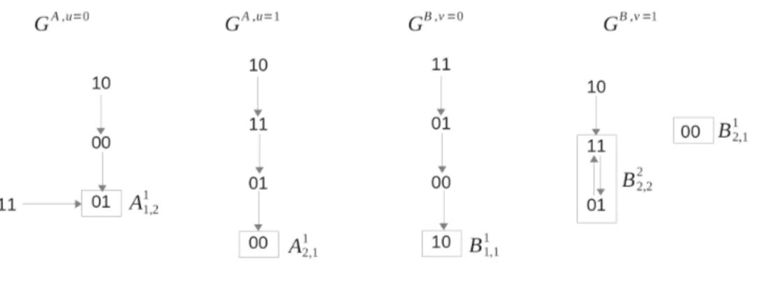
Figure 1: Example I: the asynchronous transition graphs that define the dynamics of the two systems (4). Example I. Consider the following bi-dimensional systems A and B, with nA = nB = 2 and pA =
pB = 1:
a+1 = u and (a1and nota2),
a+2 = [u and (not a1ora2)] or [not u and a1],
hA(a) = a2,
(4) b+1 = [v and not b2)] or [not v and (b1xorb2)],
b+2 = [v and b1andb2] or [not v and (b1orb2)],
hB(b) = b2,
whose asynchronous transition graphs GA,u and GB,v are shown in Fig. 1, for convenience. Note that
the attractors in all graphs are singletons except for B2
2,2 = {01, 11}. However, since the two states
have the same output (hB(01) = hB(11) = 1), in this example the semi-attractors are in fact the actual
attractors.
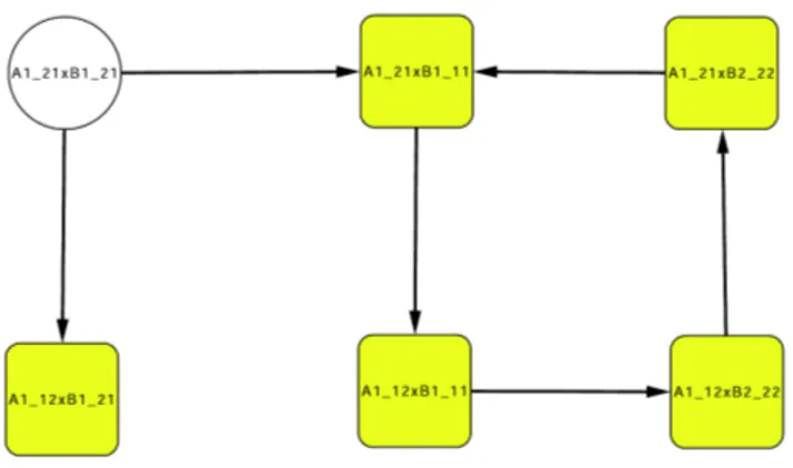
The corresponding asymptotic graph is shown in Fig. 2. To illustrate the computation of an edge, consider the product Ai
uα× B j
vβ = A121× B111 : since α = 1 = v, the system A does not induce any
change in the variables b; in contrast, the fact that β = 1 will induce a trajectory between a state in A121 and an attractor in the graph GA,2 (corresponds to Boolean input u=1). In the graph GA,2, the
state 00 is in the basin of attraction of {01} = A1
12. Therefore, there is an edge A121× B111 → A112× B111 .
All other edges are similarly computed.
Note that the full interconnected system has four variables and hence its dynamics is given by an asynchronous transition graph G with 24 = 16 states. To compute the attractors of G we needed to
compute a transition graph with only 2 × 3 = 6 states (2 attractors from system A and 3 from system B). Furthermore, as remarked above, the size of Gas can be further reduced by excluding the
cross-product states known to be transient. In this example only A1
21× B121 satisfies the condition u 6= β
and v 6= α, and can be excluded. For higher order systems, such a size reduction can represent very significant savings in computational cost.
The Gasof Example I has two attractors: Q
1= {A112× B211 } and Q2= {A112× B111 , A112× B222 , A121×
B1
11, A121× B222 }. For this 4-dimensional example, it is easy to check that Q1 is a true attractor of the
full interconnected system (see also Prop. 1), while Q2 is a “spurious” attractor, that is, not a real
attractor of G. To see this, it suffices to note that there is a pathway that leads from a state within Q2
to Q1, and which is not “covered” by Gas:
Q2∋ A121× B222∋ (00, 01) GB,1
−→ (00, 00)G−→ (01, 00) ∈ QA,1 1
This Example shows that even very simple (and deterministic) individual asynchronous dynamics can lead to asymptotic graphs that exhibit spurious attractors. However, note that this example was specif-ically contrived to illustrate the generation of spurious attractors; its Boolean rules are not necessarily biologically plausible.
Figure 2: Example I: the asymptotic graph of the interconnection of the two systems (4). The cross-products inside shaded squares belong to an attractor. The cross-product inside a white circle represents a transient state that can be excluded from the computation.
In view of Example I, it would be useful to complement Theorem 1 by conditions permitting to decide whether an attractor of Gas is also an attractor of G. An exact result was also proved in [23] –i.e.,
recovering exactly all the attractors in G from the cross-products of semi-attractors, with no spurious generation,– by computing the cross graph which is similar to Gas but involves cross-products of all
(semi-)SCCs (as opposed to considering only semi-attractors). However, depending on the number of
SCCs, the cross graph can often be more costly to compute than the full graph G, hence the usefulness of establishing sufficient conditions for deciding whether an attractor of Gas is a “true” attractor.
Some preliminary results were presented in Proposition 1 of [23], which are improved below in Prop. 1. To state this, we need to introduce projection functions, for V = Ai
uα× B j vβ, and R = {V1, . . . , Vr}: π(V ) = {(a, b) ∈ Ω : a ∈ Ai uα, b∈ B j vβ}, π(R) = ∪V ∈Rπ(V ),
πA(R) = {a ∈ ΩA: ∃b such that (a, b) ∈ π(R)}.
The A-output of R is the set:
A-output = {hA(a) : a ∈ πA(R)} ⊂ HA
Similar definitions apply for the projection πB(R) and the B-output of R.
Recall that we are assuming qA= pBand qB= pA, hence HA≡ UB and HB ≡ UAand the A-output
(resp., B-output) of R is also contained in UB (resp., UA). The new result of Prop. 1 is in parts (ii),
(iii), which previously stated “for all u ∈ UA” or “for all v ∈ UB”. The new conditions are much less
restrictive, although the proof is similar. If Proposition 1 is not applicable, then one may still verify a
posteriori whether R represents an attractor of G by simulating all trajectories starting from all states
in π(R) and checking whether any of them leaves R (however, this “direct force” procedure may also involve some computational costs).
Proposition 1 Let R be a terminal SCC of Gas. If either one of the following conditions is satisfied:
i) R is a singleton (i.e., contains a single product V );
ii) the A-output of R is a singleton and the set πA(R) is an attractor of GA,ufor all u in the B-output
of R;
iii) the B-output of R is a singleton and the set πB(R)} is an attractor of GB,v for all v in the
A-output of R;
Proof: We will use the notation (a, b) ❀G (a′, b′) to denote a path connecting the two elements in the
transition graph G and (a, b) →G(a, b′) to denote a one-step transition.
Part (i) is unchanged from [23]. Parts (ii) and (iii) are very similar, so we will only prove part (iii). If the B-output of R is a singleton, say {α}, then any V ∈ R must be of the form
Ajα(·)× Bvα(·), for some v in the A-output of R.
In particular, (see definition of semi-SCC) all Ajα(·) belong to the same attractor Aj
αof GA,α.
Suppose now that the set πB(R) is an attractor for all v in the A-output of R. Then, to show that
π(R) is an attractor of Gas, it suffices to show that: (1) π(R) is a strongly connected set, and (2) π(R)
contains all its successors. If (1) and (2) hold, then π(R) is indeed a terminal SCC. To show (1), let (a, b) and (a′
, b′
) be any two elements of π(R). Then
(a, b) ❀G(a, b′), since πB(R) is an attractor of GB,hA(a)(v = hA(a) ∈ A-output)
(a, b′
) ❀G(a′, b′), since a, a′ belong to the same attractor Ajα of GA,α.
To show (2), observe that there are two forms of successors: either (a, b) →G(a′, b) or (a, b) →G(a, b′).
We want to prove that both (a′
, b) and (a, b′
) are in π(R). In the first case, since a, a′
belong to the same attractor Aj
α, it is immediate to see that (a ′
, b) ∈ π(R). In the second case, since b′
∈ πB(R) and
πB(R) is an attractor of GB,hA(a), by definition of πB(R) there some exists a′such that (a′
, b′) ∈ π(R).
Recall that the B-output is a singleton so hB(b′) = α. This implies
(a, b′
) ❀G (a′, b′) ❀G(a, b′), since a, a′ belong to the same attractor Ajαof GA,α.
Therefore, (a, b′) ∈ π(R) as wanted.
Remark. The generalization of points (ii) and (iii) of Proposition 1 to multiple A-outputs and B-outputs is not clear, due to Example I where the spurious attractor Q2 satisfies
A-output=B-output={1,2}. Other examples exist where an attractor of Gas of the same form as Q
2 is indeed
and attractor of G (see Example 2 in [11]).
If Proposition 1 cannot be applied, there may be other methods to decide whether an attractor of Gas is a true attractor, such as identifying invariant sets of the system that contain the given attractor:
examples of this are given below in Propositions 3 and 4.
Example II.To illustrate the relevance of Prop. 1, another theoretical example is now given. The two systems A and B are more conveniently represented by their asynchronous transitions graphs, one for each fixed input (Fig. 3). The dimensions are na = 2, nB = 3, pA = 1, pB = 2 and their outputs
are as follows:
hA(a) = (a1, a2)′, hB(b) = b1.
Note that attractor A1
2 splits into two semi-attractors, A121 and A223, and the attractor B12 splits into
B211 and B222. The full interconnected system has five variables and hence its dynamics is given by an
asynchronous transition graph G with 25 = 32 states. To compute the attractors of G we needed to
compute a transition graph with 4 × 7 − 8 = 20 states: 4 semi-attractors from system A and 7 from system B, and 8 transient cross-products (see also Fig. 4).
The Gas of Example II (Fig. 4) has two attractors: Q
1= {A111× B111 } and Q2= {A121× B321 , A121×
B2
12, A223× B121 , A223× B321 }. It is easy to check that Q1= {00000} is an attractor of G, by Prop. 1(i).
Likewise
Q2= {10111, 10101, 10100, 00111, 00101, 00100}
is also an attractor of G, by Prop. 1(iii): the B-output is a singleton since {hB(b) : b ∈ πB(Q2)} = {1};
the A-output of Q2is {hA(a) : a ∈ πA(Q2)} = {10, 00}; and, finally, the set πB(Q2) = {111, 101, 100}
Figure 3: Example II: the asynchronous transition graphs of systems A and B, for each fixed input.
Figure 4: Example II: the asymptotic graph of the interconnection of systems A and B defined in Fig. 3. States inside light shaded squares belong to some attractor; there are two attractors in this graph. States inside white circles represent known transient state, which can be discarded from the computation. States inside light shaded circles represent all other states.
3
Application: a model for E. Coli growth mechanism
The bacteria Escherichia Coli are unicellular micro-organisms (present in the human gut, for instance) which grow and divide in the presence of a carbon source, such as glucose or other sugars. In typical experiments, in a carbon rich medium, the bacteria are observed to grow at a constant growth rate, which is referred to as the exponential phase [25]. In the absence of carbon, the bacteria enter a
stationary phase, with no cellular growth or division. E. Coli use a network of genes and proteins
to detect the presence or absence of carbon sources and respond accordingly, by adjusting their gene expression levels.
The major players in this nutritional response network are well characterized (see, for instance, [16, 19, 18] and references therein) but, in contrast, it has been difficult to find an appropriate dynamical expression for modeling the growth rate of E. Coli [25]. In other words, if one wishes to add a model variable to describe growth rate, what should its mathematical rule be? To overcome this problem, models often focus on either the exponential or the stationary phases, thereby considering growth rate to be either constant or zero, respectively [20]. However, such models are not able to describe the transition from one phase to the other, thus failing to provide intuition on a crucial cellular mechanism. Growth should depend on the capacity of the bacteria to produce all the different proteins nec-essary to its development and cellular division. In its turn, the synthesis of any protein depends on the transcription and translation steps, which are limited, respectively, by the concentrations of RNA polymerase and ribosomes. To model the many proteins involved in bacterial growth, we will therefore distinguish between three “classes”: RNA polymerase, ribosomal proteins, and all others will be col-lectively denoted as “bulk” proteins (as a reference see also [17], where a distinction is made between ribosomal and nonribosomal proteins). Some models have thus tried to include these effects to obtain a more accurate expression for growth rate. For instance, one may have a dependence on one step:
Growth rate ∼ RNA polymerase (5) as tested previously in [26], or in two (or more) steps, each of them separately limiting growth rate, hence the use of the minimum function:
Growth rate ∼ min{ ribosomal proteins, bulk proteins } (6) as considered in [17], or
Growth rate ∼ min{ ribosomal proteins, RNA polymerase } (7) as we considered in [27]. In this Section, our goal is to test these expressions, by interconnecting a well known nutritional response module with a basic transcription/translation model, using the Boolean interconnection method described in Section 2.3.
3.1
E. Coli nutritional stress response module
The nutritional stress response network developed in [18] involves three groups of variables, each repre-senting a different regulatory effect: DNA supercoiling (determined by the enzymes GyrAB and TopA), carbon response (involving the proteins Crp, Cya), and a global regulator (protein Fis) that sends the carbon availability signal down to the stable RNAs (rrn). The latter are limiting factors in ribosome production, and are thus a measure of the growth of the bacteria.
A very brief description of the main biological steps in response to nutritional stress is as follows (see [18] and references therein): in answer to carbon depletion, the bacteria increase their cyclic AMP concentration (cAMP); this small molecule will bind to Crp (cAMP receptor protein) to form a complex that controls the expression of different genes, some involved in the synthesis of enzymes that allow the bacteria to make use of other carbon sources, others involved in morphological changes and motility. The complex cAMP-Crp also activates the enzyme Cya (adenylate cyclase), which contributes to produce cAMP from ATP, and represses the global regulator Fis, a protein which is available at high concentration during the exponential phase, and is responsible for the control of many other genes. The protein Fis also represses the complex cAMP-Crp and, among others, it controls two enzymes
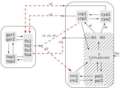
gyr1 gyr2 fis1 fis2 fis3 fis4 top1 top2 crp1 crp2 cya1cya2 rrn1 rrn2 pol1 pol2 µ fg(rrn,pol,crp) W1 W2 qy qr v1, v2, v3 u3 u2 u1 v3 Glu
Figure 5: The interconnection of the fis global regulatory module (left rectangle) and a basic cellular growth model (right rectangle). Each module has three inputs and outputs: u = (u1, u2, u3), v =
(v1, v2, v3). The dashed lines represent the interconnection: i.e., the output of one system becomes the
input of the other. Bacterial growth rate is internally computed as a function of the external nutrient sources (Glu), ribosomes (here represented by rrni), RNA polymerase (poli) or “bulk” proteins (which
will be basically represented by crp). Growth rate is first translated into two qualitative levels, W1and
W2, which signal downstream. The region under hatching represents the new variables and interactions
involved in DNA topology regulation: Gyrase AB (GyrAB) which induces negative supercoils in the DNA and Topoisomerase A which restores supercoiling to “normal” levels. Finally, Fis also stimulates the transcription of stable RNAs, a necessary condition for the production of ribosomes and hence necessary for bacterial growth.
The model developed in [18] includes a constant external input named “Signal” that represents nutritional stress, that is, the presence (“Signal”= 0) or absence (“Signal”= 1) of carbon sources, while the variable rrn is simply an output, as it does not influence the other variables. Growth rate was summarized into the effect of the complex cAMP-Crp on the other variables, namely Fis, Crp, and Cya. Depending on the value of “Signal”, the network reproduced two steady states corresponding to the stationary or exponential phases of E. coli, characterized in Table 1. The two states predicted by this model are consistent with experimental observations: in the exponential phase, Fis is present at high levels, as well as stable RNAs, and the cAMP receptor protein is not strongly present. The opposite happens in the stationary phase.
In our model, the interactions are reorganized in order to include the explicit effect of growth rate. It is known that the complex cAMP-Crp is growth dependent [28], so we replaced this complex by an equivalent expression that depends on Crp, Cya, and growth, now represented by the arrows u1, qrand
qy in Fig. 5. The components inside the hatched region in Fig. 5 were not present in model [18], and
the rrn variable did not influence the system. The objective in this paper is thus to refine the effect of growth in the system, as described below in Section 3.2.
The model [18] consists of a piecewise affine system on six variables, it was further studied in [29, 30, 31] and has been written as an extended Boolean model in [21], using the procedure briefly described in Section 2. The first Boolean module is formed by the 8 variables corresponding to genes fis, gyr, and
top, since fis is described by 4 Boolean variables and gyr, top by 2 each (see Fig. 5). The rules for this
module are given in the Appendix.
Since each variable may have several discrete values, the Boolean models will use vari, i ∈ {1, 2, . . . , d}
to denote the corresponding d Boolean variables (see Section 2.1) (similarly for the other variables). The discrete variable can be recovered simply by adding the Boolean variables:
var =
d
X
i=1
vari. (8)
Table 1: The two E. coli modes reproduced by the model [18]. If a variable has more than one value, this means that the asymptotic solution is oscillatory among those values.
“Signal” fis gyr top crp cya rrn Phase 0 1,2,3,4 1,2 0 1 2 0,1 Exponential 1 0 2 0 2 2 0 Stationary
3.2
The cellular growth module
To test the dependence of growth rate on some of the major model components, we will study a “closed-loop system”: that is, use the state of the system to construct a mathematical expression for bacterial growth rate and then feed it back to the system, by letting proteins Cya and Crp depend on it. Thus, cellular growth rate (represented by µ) now appears explicitly in the model, as an internal variable that depends dynamically on the state of the system at each instant (see Fig. 5). In agreement with the variables of the system, growth rate will have two positive discrete levels (translated to W1and W2, see
equation (9) below). This also implies that the effect of growth on fis, crp and cya has to be updated relative to the original model [18]. In Fig. 5, there are thus three links (respectively, u1, qrand qy) which
are not fixed for now, but for which several possible combinations will be tested, with a view to better understand growth signaling (see Section 4). The motivation for building this closed-loop system is to test the dynamical dependence of bacterial growth rate on the system’s variables, a question which is
still not well understood. Thus, for this example, an expression for growth rate will be considered valid
if the refined system in Fig. 5 is able to reproduce the same results as the (more schematic) model [18].
As indicated in Fig. 5, the second Boolean module will describe the expression of the genes encoding for crp, cya, rrn, and will further include pol, to represent the expression of RNA polymerase, the enzyme responsible for gene transcription (2 Boolean variables each). The presence of carbon sources will be represented by the external input Glu. Previously [26], we have studied a mathematical expression for bacterial growth rate that is dependent only on RNA polymerase, for a simple 2-dimensional model. However, experimental data [17] suggests that ribosomes play a major role, hence we wish to improve our results by analyzing models that consider different combinations of limiting factors, and checking their compatibility with known results.
The growth variable, µ, and its downstream signals will be given by:
µ = Glu and fg(rrn1,rrn2,pol1,pol2,crp1,crp2); (9)
W = 2 − µ; W1 = sign(W );
W2 = max(0, W − 1);
where sign(W ) = 1 if W > 0 and sign(W ) = 0 if W = 0 (by construction, sign(W ) is never negative). The variables W1 and W2 correspond, respectively, to:
W1= 1 ⇔ µ ≤ 1, W2= 1 ⇔ µ = 0.
and satisfy W1≥ W2. Following (5)-(7) and (8), different expressions for the function fgwill be tested,
namely:
fgr = rrn1+ rrn2,
fgp = pol1+ pol2,
fgb = crp1+ crp2, (10)
frp
g = min(rrn1+ rrn2,pol1+ pol2)
fgrb = min(rrn1+ rrn2,crp1+ crp2),
where the protein Crp is used as a surrogate for the level of expression of “bulk” proteins. In addition, to describe how the growth rate affects the genetic machinery, two functions need to be chosen: these correspond to the arrows labeled qy and qr (see below), which will also be a function of W1 and W2.
Several possible combinations will be tested and the final results compared to the original model.
3.3
System interconnection
The full discrete system will thus have 7 variables,
V = (fis, gyr, top, crp, cya, rrn, pol)′
, with discrete levels d1= 4, dj = 2 for j = 2, . . . , 7 and state space:
Ωd= {0, 1, . . . , 4} × {0, 1, 2} × . . . × {0, 1, 2}.
The extended Boolean model will have 16 variables. As described in Section 2.3, the interconnection of two input/output asynchronous Boolean networks such as systems (13) and (14), is obtained by setting u= hB(b) and v = hA(a). Most of the input/output functions are already fixed by model [18]. There
is a new interaction between the two modules, due to the effect of the growth rate in fis, which is represented by u1 in Fig. 5: u1∈ {W1, W2}, u2= crp1 or crp2, u3= cya1 or cya2, v1= fis1, v2= fis2 or fis4, v3= fis3.
The goal in this paper is the discrimination between different variants of the model in Fig. 5, in order to choose the mechanism that better represents bacterial response. The variants cover:
• models for growth rate: fr
g, fgb, fgrb, and fgrp;
• interactions between growth signals and the genetic machinery response: qr, qy, and u1.
As remarked above (Section 3.1), the interactions qr, qy, and u1 in some sense replace the effect of the
complex cAMP-Crp on the system, by including an explicit dependence on growth rate. To evaluate the new rules we will consider that there are two signaling stages, corresponding to the response of Cya/cAMP (the initial steps in the case of nutritional stress) and of Fis (global regulator). The response of crp will be timed with one or the other:
qr= u1 or qr= qy.
The following distinct combinations for qy, qr and u1 will be tested:
(I) qy= W1, qr= W1, u1= W1 (II) qy= W1, qr= W1, u1= W2 (III) qy= W2, qr= W2, u1= W1 (11) (IV ) qy= W1, qr= W2, u1= W2 (V ) qy= W2, qr= W2, u1= W2 (V I) qy= W2, qr= W1, u1= W1
4
Results
As discussed above (cf. Section 3), the goal is to recover the behavior of the system as described in Ropers et al [18] (Table 1) but now with growth rate “actually computed” by the bacteria, for the system in closed loop form which uses the state of the system. Various combinations of interactions and growth rate functions were tested, with the results summarized in Table 2 and discussed below.
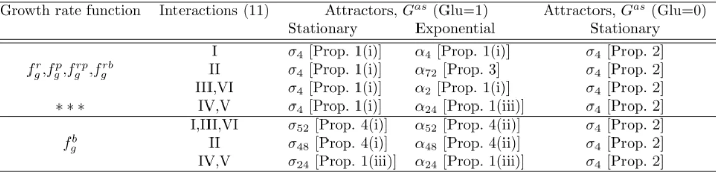
Table 2: The attractors for each combination of growth rate function and interactions u1, qr, qy.
Attractors σi satisfy rrn = pol = 0, while attractors αj, j ∈ {2, 4, 24, 48, 52, 72}, satisfy rrn ≥ 1 and
pol ≥ 1 (full characterizations are given in Sections 4.2 and 4.3). The indexes i, j denote the number of
distinct states contained in the attractor. All the attractors of Gasare also attractors of G: either they
satisfy Prop. 1 and/or other methods, as indicated. The highlighted row (∗ ∗ ∗) represents the model variants which better reproduce Table 1 results (see Section 4.4).
Growth rate function Interactions (11) Attractors, Gas (Glu=1) Attractors, Gas (Glu=0)
Stationary Exponential Stationary
fr
g,fgp,fgrp,fgrb
I σ4[Prop. 1(i)] α4[Prop. 1(i)] σ4[Prop. 2]
II σ4[Prop. 1(i)] α72[Prop. 3] σ4[Prop. 2]
III,VI σ4[Prop. 1(i)] α2[Prop. 1(i)] σ4[Prop. 2]
∗ ∗ ∗ IV,V σ4[Prop. 1(i)] α24[Prop. 1(iii)] σ4[Prop. 2]
fb g
I,III,VI σ52[Prop. 4(i)] α52[Prop. 4(ii)] σ4[Prop. 2]
II σ48[Prop. 4(i)] α48[Prop. 4(ii)] σ4[Prop. 2]
IV,V σ24[Prop. 1(iii)] α24[Prop. 1(iii)] σ4[Prop. 2]
As an indication of the computational costs, application of the method presented in Section 2.3 to compute the attractors for model frp
g , case IV, gave the following results:
• there are eight constant-input asynchronous transition graphs for each system (GA,u, or GB,v);
• on these graphs there are a total of 22 semi-attractors for system ΣA and 20 for ΣB;
• as remarked in Section 2.3 (and [23]), the number of vertices in Gas can be further reduced by
eliminating those which are known to have no incoming arrow. This leads to only 90 vertices; • the computational cost of finding the attractors of the interconnected system Σ has therefore been
reduced from analysis of a size 216= 65536 to a size 90 matrix;
• one should nevertheless consider the cost of computing this size 90 matrix, which involves reach-ability calculations in the 2 × 8 individual asynchronous transition graphs (the full process was very fast here, taking between 30-60 seconds for each model variant).
4.1
General properties
Some immediate observations from the results are:
• a common point to all model variants is that, in the presence of nutrient (Glu=1), Gas always
has two attractors which are both attractors of G, by application of Prop. 1(i) or (iii), or other methods (see Prop. 3, 4).
• for all model variants, the first attractor (σi, i ∈ {4, 24, 48, 52}) has rrn = pol = 0 and the second
attractor (αj, j ∈ {2, 4, 24, 48, 52, 72}) rrn = pol = 1. The first may be said to represent stationary
phase, while the second stands for exponential phase.
• also for all model variants, in the absence of nutrient (Glu=0), there is only one attractor, σ4;
this can be verified directly (see Prop. 2 below). The stationary phase attractor σ4has four states
and is characterized by:
σ4: fis = 0, gyr ∈ {1, 2}, top = 0, crp = 2, cya ∈ {1, 2}, rrn = 0, pol = 0. (12)
coinciding with the stationary attractor of model [18] (see Table 1) with the exception of gyr and
cya which oscillate between 1 and 2 (instead of being fixed at 2).
• all models involving the ribosomes or RNA polymerase as a growth rate limiting factor exhibit the same stationary phase and a similar exponential phase attractors, depending only on the choice of feedback interactions.
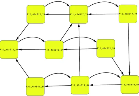
As an example, for model variant frp
g , case IV, the basins of attraction for σ4 and α24 are
dis-connected. The stationary phase attractor is formed of a single vertex, while the exponential phase attractor is composed of 9 vertices, as shown in Fig. 6. However, all system B semi-attractors coincide (Prop. 1(iii) is satisfied):
B5412= B7417= B1984= {10111010},
while the A system semi-attractors are characterized by the levels of fis, with either fis = 1,fis = 2 or f is≥ 3:
A1045 = {10000000, 10000010, 10001000, 10001010, 10001100, 10001110}, A1147 = {11000000, 11000010, 11001100, 11001010, 10001100, 11001110},
A1248 = {11100000, 11100010, 11101100, 11101010, 11101100, 11101110, 11110000, 11110010, 11111100, 11111010, 11111100, 11111110} .
In practice, the attractor in Fig. 6 can be reduced to (either) one of the horizontal rows, with three components only. All concentrations are fixed, except for fis, gyr, and top which are allowed to oscillate in any given increasing or decreasing order, provided that fis ≥ 1 and top ≤ 1.
In the case where no carbon sources are present, it can be shown that all model variants become the same, and hence exhibit the same stationary phase attractor. This is essentially due to the direct effect of growth rate on the synthesis of RNA polymerase.
Figure 6: The exponential growth phase attractor (model frp
g , case IV). Since the B j
α4components are
all equal, this attractor can be reduced to (either) one of the horizontal rows, with three components only (see text for more details).
Proposition 2 Assume that Glu=0. Then, the asymptotic graph for all model variants exhibits only one attractor, σ4.
Proof : In the case Glu=0, we immediately have the steady state values for rrn and pol:
µ= 0 ⇒ pol1= pol2= 0 ⇒ rrn1= rrn2= 0
For the interactions W , qy, qr, and u1it also follows that:
W1= W2= 1 ⇒ qy = qr= u1= 1.
Together with the rules in Appendix, this leads to:
cya1= crp1= 1 ⇒ u2= u3= 1 ⇒ fisi= hfi
which simplifies to
fis+1 = f is2, fis+2 = f is3, fis+3 = f is4, fis+4 = fis3 and not fis4.
Thus, at steady state, the values for fis satisfy fisi= 0, for all i, which in turn imply that all the outputs
of system A are zero: vi= 0 for all i. The remaining concentrations can now be easily established from
the Boolean rules, so it follows that there is only one attractor and that it is σ4 (12).
4.2
Growth Rate limited by ribosomes or RNA polymerase
For the model variants using fr
g, fgp,fgrp, or fgrb, the stationary phase attractor σ4 is always the same
wiring and has j states characterized by :
α2: fis = 0, gyr ∈ {1, 2}, top = 0, crp = 2, cya = 2, rrn = pol = 1,
α4: fis = 0, gyr ∈ {1, 2}, top = 0, crp = 2, cya ∈ {1, 2}, rrn = pol = 1,
α24: fis ∈ {1, 2, 3, 4} gyr ∈ {1, 2}, top = 0, crp = 1, cya = 2, rrn = pol = 1,
α72: fis ∈ {1, 2, 3, 4}, gyr ∈ {0, 1, 2}, top = 0, crp ∈ {1, 2}, cya ∈ {1, 2}, rrn = pol = 1.
Note that cases IV and V (α24) are similar to the exponential phase attractor of [18] (see Table 1) (the
only difference is rrn now fixed at 1, which seems reasonable for the exponential phase). Cases I,III,VI (α2,α4) fail to reproduce the levels of fis during exponential phase (here they are fixed at zero). Case II
(α72) also exhibits oscillations in crp and cya, which are not observed in Table 1. This attractor does
not fit into Proposition 1, but an alternative way to show that it is not a spurious attractor, is to note that the set of states with ribosomes, RNA polymerase and Fis all at discrete level 1 is invariant, so trajectories cannot leave this set; therefore, an attractor with such properties must exist, with the only possible candidate being α72.
Proposition 3 Assume that fg∈ {fgr, fgp, fgrp, fgrb}. The set Q = {x ∈ Ωd: rrn = 1, pol = 1, fis ≥ 1}
is invariant.
Proof : From the Boolean rules (see Appendix), it suffices to note that:
rrn = pol = 1 ⇒ µ = 1 ⇒ W1= 1, W2= 0 ⇒ qy= qr= 1, u1= 0
and also
rrn = pol = 1, µ ≥ 1 ⇒ rrn = pol = 1.
And then:
u1= 0 ⇒ fis1= h01 ≡ 1 ⇒ fis ≥ 1.
Therefore, the set Q is invariant.
4.3
Growth Rate limited by bulk proteins
For the model variants using fb
g, the exponential phase attractors are characterized as follows:
α24: fis ∈ {1, 2, 3, 4} gyr ∈ {0, 1, 2}, top = {0, 1}, crp = 1, cya = 2, rrn = pol = 1,
α48: fis ∈ {1, 2, 3, 4} gyr ∈ {0, 1, 2}, top = {0, 1}, crp ∈ {1, 2}, cya = 2, rrn = pol = 1,
α52: fis ∈ {0, 1, 2, 3, 4}, gyr ∈ {0, 1, 2}, top = {0, 1}, crp ∈ {1, 2}, cya = 2, rrn = pol = 1.
The stationary phase attractors are similar in all variables except that rrn = pol = 0. Comparison with Table 1 shows many differences with respect to model [18]. These attractors are also true attractors of G, as shown by application of the following result.
Proposition 4 Define the sets P0 and P1:
P0= {x ∈ Ωd: rrn = 0, pol = 0}, P1= {x : rrn = 1, pol = 1}.
Then:
(i) The set P0 is invariant independently of the function fg;
(ii) The set P1 is invariant if fg= fgb.
Proof : Invariance of P0 follows directly from the Boolean rules for rrni and poli. For P1, it suffices to
note that the Boolean rules imply (see Appendix): cya ≥ 1 and crp ≥ 1 which imply µ ≥ 1. Then,
4.4
Model discrimination
Based on the observations above and comparison of Tables 1 and 2, it seems clear that the growth rate function should depend on the ribosomes and/or RNA polymerase. With this model, at steady state there is no difference between a dependence on ribosomes or RNA polymerase, although the transient dynamics do depend differently on these two species (simulations in Section 4.5). (This may be due to a very simplified model for the transcription/translation steps which is, however, not our aim to study here.) The model variants corresponding to I,III,VI do not satisfy the properties of the exponential phase attractor and can thus be eliminated. The interconnection of type II has most of the correct properties, but it allows the concentration of crp and cya to oscillate, in contrast to the original model. The cases that better fit the original model are IV and V, whose asymptotic behavior is indistinguishable. This is consistent with the observations (summarized in Ropers et al. [18]) that: immediately upon carbon starvation, or absence of carbon source, transcription of the gene cya is activated, which leads to production of the protein Cya. Phosphorylation of Cya leads to synthesis of cyclic AMP, which in turn will bind to Crp and produce a complex [cAMP-Crp]. This complex will then control a variety of genes which are directly involved in the adaptive response of E. coli to a deprivation of carbon. Among others, it activates crp, and inactivates cya and the global regulator fis.
Furthermore, to establish the transition to exponential phase, and guarantee the presence of global regulator fis, the wiring interactions should be as in cases II, IV, and V, which all satisfy u1 = W2:
in other words, since W2 = 1 corresponds to µ = 0, fis is inhibited only at low growth rate, as also
observed in [18]. The levels of crp and cya are in agreement with those of Table 1 if crp is activated at high growth rate level and the inhibition effect on cya is not later than the activation of crp, i.e., qr= W2, qy ≥ qr (recall that W1≥ W2).
In conclusion, to develop a more detailed continuous model, bacterial growth rate should depend on the ribosomes. For simplicity, one may even consider the ribosomes to be the only variable influencing growth rate (besides the external input), because no differences were observed between models with fr
g,
fgrp, or frb g .
4.5
Dynamical behavior
By virtue of Theorem 1 and Propositions 1 to 4, we know that any trajectory of the interconnected model will eventually reach either the exponential or stationary phase attractors, depending on the initial condition and path in the graph G. To illustrate possible dynamical behaviors, we can generate trajectories in G, by randomly choosing the variable to be updated at the next instant, according to the rules. Note that this simulation does not need the graph G to be constructed; but, on the other hand, such simulations cannot characterize the full behavior of the network. Hence the usefulness of the asymptotic graph Gas, which can now be completed with some statistical results on initial conditions
and attractors reached.
For the statistical analysis we choose interconnection model IV, and growth rate models frp
g , fgr, and
fp
g. It must be noted that the asymptotic graph “looses” some trajectories of the full interconnected
system as, to construct Gas, the system is assumed to evolve in one of the
constant-input/constant-output graphs {a}×GB,αor GA,β×{b} until reaching an attractor. In simulations, however, the system
is allowed to switch before reaching an attractor, meaning that the basins of attraction are not really disconnected as might be suggested by the asymptotic graph.
Monte Carlo simulations of the full model (104 randomly generated trajectories) assume that all
transitions in G are equally probable and show that the two attractors are reached with similar fre-quencies: for frp
g , a fraction of 0.59 (0.57 for fgr, or 0.58 for fgp) trajectories converge to the exponential
phase attractor.
Note that the invariance results in Propositions 3 and 4 already provide an idea of the basins of attractions, since they imply notably that initial conditions of the form rrn = pol = 0 (resp.,
rrn = pol = 1) lead immediately to the stationary (resp., exponential) phase attractor. To obtain more
information on the distribution of the basins of attraction, we have further analyzed the probability that the system converges to either attractor given an initial condition with variable vari = ℓ (where vari
runs over the sixteen Boolean variables of the system and ℓ ∈ {0, 1}). We found that the convergence to either attractor depends essentially on the initial concentrations of RNA polymerase and ribosomes,
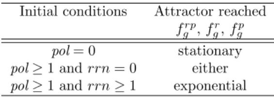
while all other concentrations play minor roles (in agreement with Propositions 3 and 4). An interesting observation is that, for all variables except the polymerase, and for any initial condition, the probability of converging to exponential phase is higher than to stationary phase. It is also evident that the absence of polymerase immediately prevents convergence to exponential phase. In addition, we observe that all trajectories converging to exponential phase need to start with an intermediate (or higher) level of RNA polymerase (pol ≥ 1). Table 3 summarizes the statistics obtained from the Monte Carlo simulations. Our studies lead to the conclusion that RNA polymerase and ribosomes are both crucial for bacterial
Table 3: Initial conditions and attractor reached, for some model variants, with interconnection of type IV.
Initial conditions Attractor reached frp
g , fgr, fgp
pol = 0 stationary
pol ≥ 1 and rrn = 0 either
pol ≥ 1 and rrn ≥ 1 exponential
growth, but exert their roles at different times: initially, the presence of RNA polymerase is necessary to grow and reach the exponential phase (otherwise, if RNA polymerase is absent at time zero, the bacteria enter the stationary phase even in the presence of carbon sources), while ribosomes can be absent; at later times, the presence of ribosomes is essential to guarantee the entry into exponential phase.
5
Conclusions
Several dynamic model variants for bacterial growth rate that consider limitation by availability of the proteins needed for cell division (RNA polymerase for transcription, ribosomes for translation, or other “bulk” proteins) were tested and compared to a well established model. The main goal was to analyze (qualitative) feasibility of the wiring network, as well as the logical coherence of each model variant. This was accomplished by using a Boolean version of the model for nutritional stress response in [18], coupled with a basic cellular growth module.
We can conclude that Boolean models provide a useful framework for analysis of a system’s dynamical behavior, convenient for hypotheses testing and model discrimination. This framework presents several advantages from a computational point of view, as many tools and algorithms are available for the study and rigorous analysis of the networks. In particular, using the interconnection of two Boolean modules, it is possible to compute the attractors of a large network at a much lower cost than with classical graph theoretical tools. However, the drawbacks of this methodology include problems related to identifying the two (or more) Boolean modules as well as the corresponding inputs and outputs, which are not always obvious (see also [23]). As the number of modules and inputs increases, also the computational cost will increase and a balance must be found. This is a topic that should be further developed in future work.
A number of interesting points arise from our qualitative analysis. First, it was clear that limitation of growth rate by the ribosomes is needed in order to correctly reproduce the asymptotic modes, as well as transient dynamics, of the original model [18]. Second, in the presence of nutrient, our closed-loop model –where bacteria internally compute their growth rate, rather than responding to an already fixed signal– has the capacity for bistability (i.e., two asymptotic modes, representing exponential and stationary phases). Thus the closed-loop model also recovers the correct response to initial conditions: if both ribosomes and RNA polymerase concentration is very low, then the bacteria cannot grow even in the presence of nutrient. In the absence of nutrient, only the stationary phase attractor remains, as should be expected. Finally, by comparison to [18], we were able to discard most of the model variants and retain several properties necessary to reproduce the original model’s attractors.
Since our main goal was essentially theoretical, we have not fully explored the directions for model im-provement suggested by our analysis. For instance, a more detailed module for transcription/translation
including other components besides ribosomes and RNA polymerase, or the modeling of the “bulk” pro-teins in a more precise way. To conclude, although discrete models are, of course, not appropriate for a detailed description of a system or to answer more specific questions, this analysis constitutes a very useful preliminary study of growth rate models. It provides many indications and clues for future work on constructing a more detailed, continuous model of the system.
Acknowledgments
We are especially grateful to Laurent Tournier for many discussions and for providing part of the Matlab codes used here to analyze the asynchronous transitions graphs (specifically, the decomposition into strongly connected components and subsequent hierarchical organization). We also thank Jean-Luc Gouz´e and our reviewers for many useful suggestions that helped improve the paper.
This work was supported in part by projects GeMCo (ANR 2010 BLAN0201-01) and ColAge (Inria-INSERM large scale initiative action).
A
Boolean rules of the two E. coli modules
The Boolean model for the Fis module is defined by a set of rules which use some auxiliary expressions of the form h− given below:
fis+1 = (not u1 and h01) or (u1 and h11);
fis+2 = (not u1 and h02) or (u1 and h12);
fis+3 = (not u1 and h03) or (u1 and h13);
fis+4 = (not u1 and h04) or (u1 and h14); (13)
gyr+1 = (not fis3 and not fis4) or (gyr2 and hf3);
gyr+2 = not fis3 and not fis4 and gyr1 and (not gyr2 or top1 or top2);
top+1 = (not fis3 and not fis4 and top2) or
(hf3 and ((not gyr2 and top2) or (gyr2 and (not top1 or top2))));
top+2 = 0.
with the auxiliary expressions:
hf2 = fis1 and fis2;
hf3 = fis1 and fis2 and fis3;
hf4 = fis1 and fis2 and fis3 and fis4;
hf4n = fis1 and fis2 and fis3 and not fis4;
h01 = 1;
h02 = (fis1 and gyr1 and not top2) or hf3;
h03 = (hf2 and gyr1 and not top2) or hf4;
h04 = hf4n and gyr1 and not top2;
h11 = ((u2 or u3) and hf2) or ((not u2 or not u3) and h01);
h12 = ((u2 or u3) and hf3) or ((not u2 or not u3) and h02);
h13 = ((u2 or u3) and hf4) or ((not u2 or not u3) and h03);
The rules for the cellular growth module can be written as follows:
crp+1 = 1;
crp+2 = (not qr and crp1 and not v1) or (qr and crp1 and not (v2 or v3));
cya+1 = 1;
cya+2 = (not qy and cya1) or (qy and (hy1 or hy2)); (14)
rrn+1 = pol1 or rrn2;
rrn+2 = pol2 and rrn1 and v3;
pol+1 = (sign(µ) and rrn1 and pol1) or pol2;
pol+2 = sign(µ) and rrn2 and pol2;
where the auxiliary expressions are
hy1 = cya1 and (not crp1 or not crp2);
hy2 = cya1 and not cya2 and crp1 and crp2;
References
[1] L. Glass, S. Kauffman, The logical analysis of continuous, nonlinear biochemical control networks, J. Theor. Biol. 39 (1973) 103–129.
[2] R. Thomas, Boolean formalization of genetic control circuits, J. Theor. Biol. 42 (1973) 563–585. [3] L. S´anchez, D. Thieffry, A logical analysis of the drosophila gap-gene system, J. Theor. Biol. 211
(2001) 115–141.
[4] R. Albert, H. G. Othmer, The topology of the regulatory interactions predicts the expression pattern of the Drosophila segment polarity genes, J. Theor. Biol. 223 (2003) 1–18.
[5] V. Sevim, X. Gong, J. Socolar, Reliability of transcriptional cycles and the yeast cell-cycle oscillator, PLoS Comput. Biol. 6 (2010) e1000842.
[6] J. Saez-Rodriguez, L. Simeoni, J. A. Lindquist, R. Hemenway, U. Bommhardt, B. Arndt, U.-U. Haus, R. Weismantel, E. D. Gilles, S. Klamt, B. Schraven, A logical model provides insights into T cell receptor signaling, PLoS Comput. Biol. 3 (8) (2007) e163.
[7] L. Calzone, L. Tournier, S. Fourquet, D. Thieffry, B. Zhivotovsky, E. Barillot, A. Zinovyev, Math-ematical modelling of cell-fate decision in response to death receptor engagement, PLoS Comput. Biol. 6 (3) (2010) e1000702.
[8] R. S. Wang, A. Saadatpour, R. Albert, Boolean modeling in systems biology: an overview of methodology and applications, Physical Biology 9 (2012) 055001.
[9] T. Cormen, C. Leiserson, R. Rivest, C. Stein, Introduction to algorithms, MIT Press and McGraw-Hill, 2001.
[10] T. Lorenz, H. Siebert, A. Bockmayr, Analysis and characterization of asynchronous state transition graphs using extremal states, Bull. Mathematical Biology 75(6) (2013) 920–938.
[11] M. Chaves, L. Tournier, Predicting the asymptotic dynamics of large biological networks by inter-connections of Boolean modules, in: Proc. 50thConf. Decision and Control and European Control
Conf., Orlando, Florida, USA, 2011.
[13] A. Gonzalez, A. Naldi, L. S`anchez, D.Thieffry, C. Chaouiya, GINsim: a software suite for the qualitative modelling, simulation and analysis of regulatory networks, BioSystems 84 (2) (2006) 91–100.
[14] A. Naldi, E. R´emy, D. Thieffry, C. Chaouiya, Dynamically consistent reduction of logical regulatory graphs, Theor. Comput. Sci. 412 (21) (2011) 2207–18.
[15] F. Fages, S. Soliman, N. Chabrier-Rivier, Modelling and querying interaction networks in the biochemical abstract machine BIOCHAM, J. Biological Physics and Chemistry 4(2) (2004) 64–73. [16] K. Bettenbrock, T. Sauter, K. Jahreis, J. Lengeler, E.-D. Gilles, Analysis of the correlation between growth rates, EIIACrr phosphorylation, and intracellular camp levels in Escherichia coli K-12, J. Bacteriol. 189 (19) (2007) 6891–6900.
[17] I. Shachrai, A. Zaslaver, U. Alon, E. Dekel, Cost of unneeded proteins in E. coli is reduced after several generations in exponential growth, Molecular Cell 38 (5) (2010) 758–767.
[18] D. Ropers, H. de Jong, M. Page, D. Schneider, J. Geiselmann, Qualitative simulation of the carbon starvation response in Escherichia coli, Biosystems 84 (2) (2006) 124–152.
[19] T. Hardiman, K. Lemuth, M. Keller, M. Reuss, M. Siemann-Herzberg, Topology of the global regulatory network of carbon limitation in Escherichia coli, J. Biotechnology 132 (2007) 359–374. [20] A. Goelzer, V. Fromion, Bacterial growth rate reflects a bottleneck in resource allocation, Biochim.
Biophys. Acta 1810 (10) (2011) 978–988.
[21] M. Chaves, L. Tournier, J. L. Gouz´e, Comparing Boolean and piecewise affine differential models for genetic networks, Acta Biotheoretica 58(2) (2010) 217–232.
[22] S. Jamshidi, H. Siebert, A. Bockmayr, Comparing discrete and piecewise affine differential equation models of gene regulatory networks, in: M. Lones, S. Smith, S. Teichmann, F. Naef, J. Walker, M. Trefzer (Eds.), Information Processing in Cells and Tissues, Vol. 7223 of LNCS, Springer, 2012, pp. 17–24.
[23] L. Tournier, M. Chaves, Interconnection of asynchronous Boolean networks, asymptotic and tran-sient dynamics, Automatica 49(4) (2013) 884–893.
[24] P. van Ham, How to deal with variables with more than two levels, in: R. Thomas (Ed.), Kinetic Logic: A Boolean Approach to the Analysis of Complex Regulatory Systems, Vol. 29 of Lecture Notes in Biomathematics, Springer-Verlag, 1979, pp. 326–343.
[25] A. Marr, Growth rate of Escherichia coli, Microbiol. Rev. 55 (1991) 316–333.
[26] A. Carta, M. Chaves, J.-L. Gouz´e, A simple model to control growth rate of synthetic E. coli during the exponential phase: model analysis and parameter estimation, in: D. Gilbert, M. Heiner (Eds.), CMBS 2012, Lecture Notes in Computer Science 7605, Springer, 2012, pp. 107–12. [27] A. Carta, M. Chaves, J.-L. Gouz´e, A class of switched piecewise quadratic systems for coupling
gene expression with growth in bacteria, in: Proc. 9thIFAC Symp. on Nonlinear Control Systems
(NOLCOS’13), Toulouse, France, 2013.
[28] S. Berthoumieux, H. de Jong, G. Baptist, C. Pinel, C. Ranquet, D. Ropers, J. Geiselmann, Shared control of gene expression in bacteria by transcription factors and global physiology of the cell, Molecular Systems Biology 9 (2013) 634.
[29] F. Grognard, J.-L. Gouz´e, H. de Jong, Piecewise-linear models of genetic regulatory networks: theory and example, in: I. Queinnec, S. Tarbouriech, G. Garcia, S. Niculescu (Eds.), Biology and control theory: current challenges, Lecture Notes in Control and Information Sciences (LNCIS) 357, Springer-Verlag, 2007, pp. 137–159.
[30] L. Tournier, J.-L. Gouz´e, Hierarchical analysis of piecewise affine models of gene regulatory net-works, Theory Biosci. 127 (2008) 125–134.
[31] F. Corblin, S. Tripodi, E. Fanchon, D. Ropers, L. Trilling, A declarative constraint-based method for analyzing discrete genetic regulatory networks, BioSystems 98 (2) (2009) 91–104.

![Table 1: The two E. coli modes reproduced by the model [18]. If a variable has more than one value, this means that the asymptotic solution is oscillatory among those values.](https://thumb-eu.123doks.com/thumbv2/123doknet/14779329.595445/12.918.250.683.749.807/table-modes-reproduced-variable-asymptotic-solution-oscillatory-values.webp)