Magnetohydrodynamics measurements in the von Karman sodium experiment

HAL Id: hal-00492374

https://hal.archives-ouvertes.fr/hal-00492374

Submitted on 15 Jun 2010

HAL is a multi-disciplinary open access

archive for the deposit and dissemination of

sci-entific research documents, whether they are

pub-lished or not. The documents may come from

teaching and research institutions in France or

abroad, or from public or private research centers.

L’archive ouverte pluridisciplinaire HAL, est

destinée au dépôt et à la diffusion de documents

scientifiques de niveau recherche, publiés ou non,

émanant des établissements d’enseignement et de

recherche français ou étrangers, des laboratoires

publics ou privés.

Magnetohydrodynamics measurements in the von

Karman sodium experiment

Mickaël Bourgoin, Louis Marie, François Pétrélis, Cécile Gasquet, Alain

Guigon, Jean-Baptiste Luciani, Marc Moulin, Frédéric Namer, Javier

Burguete, Arnaud Chiffaudel, et al.

To cite this version:

Mickaël Bourgoin, Louis Marie, François Pétrélis, Cécile Gasquet, Alain Guigon, et al..

Magneto-hydrodynamics measurements in the von Karman sodium experiment. Physics of Fluids, American

Institute of Physics, 2002, 14 (9), pp.3046-3058. �10.1063/1.1497376�. �hal-00492374�

Magnetohydrodynamics measurements in the von Ka´rma´n sodium

experiment

Mickae¨l Bourgoin

Laboratoire de Physique, UMR 5672 CNRS and Ecole Normale Supe´rieure de Lyon, 46 alle´e d’Italie, F-69007 Lyon, France

Louis Marie´

Service de Physique de l’Etat Condense´ Direction des Sciences de la Matie`re, CEA-Saclay, F-91191 Gif sur Yvette, France

Franc¸ois Pe´tre´lis

Laboratoire de Physique Statistique, UMR 8550 CNRS and Ecole Normale Supe´rieure, 24 rue Lhomond, F-75005 Paris, France

Ce´cile Gasquet

Service de Physique de l’Etat Condense´ Direction des Sciences de la Matie`re, CEA-Saclay, F-9119 Gif sur Yvette, France

Alain Guigon and Jean-Baptiste Luciani

Service de Technologie des Re´acteurs Direction de l’E´nergie Nucle´aire CEA-Cadarache, 13108 Saint Paul lez Durance, France

Marc Moulin

Laboratoire de Physique, UMR 5672 CNRS and Ecole Normale Supe´rieure de Lyon, 46 alle´e d’Italie, F-69007 Lyon, France

Fre´de´ric Namer

Service de Technologie des Re´acteurs Direction de l’Energie Nucle´aire CEA-Cadarache, 13108 Saint Paul lez Durance, France

Javier Burguete,a)Arnaud Chiffaudel, and Franc¸ois Daviaud

Service de Physique de l’Etat Condense´ Direction des Sciences de la Matie`re, CEA-Saclay, F-91191 Gif sur Yvette, France

Stephan Fauve

Laboratoire de Physique Statistique, UMR 8550 CNRS and Ecole Normale Supe´rieure, 24 rue Lhomond, F-75005 Paris, France

Philippe Odier and Jean-Franc¸ois Pintonb)

Laboratoire de Physique, UMR 5672 CNRS and Ecole Normale Supe´rieure de Lyon, 46 alle´e d’Italie, F-69007 Lyon, France

!Received 2 August 2001; accepted 7 June 2002; published 2 August 2002"

We study the magnetic induction in a confined swirling flow of liquid sodium, at integral magnetic Reynolds numbers up to 50. More precisely, we measure in situ the magnetic field induced by the flow motion in the presence of a weak external field. Because of the very small value of the magnetic Prandtl number of all liquid metals, flows with even modest Rm are strongly turbulent.

Large mean induction effects are observed over a fluctuating background. As expected from the von Ka´rma´n flow geometry, the induction is strongly anisotropic. The main contributions are the generation of an azimuthal induced field when the applied field is in the axial direction !an # effect" and the generation of axial induced field when the applied field is the transverse direction !as in a large scale$effect". Strong fluctuations of the induced field, due to the flow nonstationarity, occur over time scales slower than the flow forcing frequency. In the spectral domain, they display a f!1 spectral slope. At smaller scales !and larger frequencies" the turbulent fluctuations are in agreement with a Kolmogorov modeling of passive vector dynamics. © 2002 American Institute of Physics. %DOI: 10.1063/1.1497376&

I. INTRODUCTION

The motion of an incompressible electrically conducting fluid in the presence of an applied magnetic field is gov-erned, respectively, by the fluid and induction equations:

'u 't"!u"“"u#! “p ( ")*u" curl B (+0 ÃB, !1" div u#0, 'B 't #curl!uÃB"" 1 +0, *B, !2" div B#0,

a"_{Present address: Departemento de Fı´sica y Matema´tica Aplicada,}

Univer-sided de Navarra, E-31080 Pamplona, Spain.

b"_{Author to whom all correspondence should be addressed. Electronic mail:}

pinton@ens-lyon.fr

3046

where(,),,,+0 are, respectively, the fluid’s density,

kine-matic viscosity, electrical conductivity, and magnetic perme-ability. These equations must be supplemented by boundary conditions: no-slip for the velocity field, continuity of the electromagnetic field at the flow wall, and electrical conduc-tivity and geometry of the outer medium.1For a chosen flow geometry and wall conductivity, the control parameters of the system are the magnetic Reynolds number Rm, the

ki-netic Reynolds number Re, and the interaction parameter N:

Rm#

def_{magnetic stretching}

magnetic diffusivity-+,UL#2.+0,R

2_{#, !3"}

Re #

def_{nonlinear advection}

viscous dissipation -UL ) # 2.R2# ) , !4" N#

def_{Lorentz force}

pressure force

-,B02L

(U , !5"

where U, L are characteristic values for the flow velocity and size and B0 is the applied magnetic field. In the cylindrical

geometry used in this study—see Sec. II—the characteristic size is the cylinder radius R and the characteristic velocity is the driving disk speed U#2.R#, where # is the rotation

rate. The ratio of the magnetic to kinematic Reynolds num-ber is the magnetic Prandtl numnum-ber

Pm#+,)# Rm

Re. !6"

It is very small !less than -10!5" for all liquid metals. Note that once the nature of the conducting fluid is chosen, Eq. !6" gives a fixed relationship between the kinetic and magnetic Reynolds numbers which can no longer be set independently. There have been numerous studies of the influence of a strong magnetic field on weak flows of an electrically con-ducting fluid, i.e., in the parameter range N$1, Rm%1.2 In

this case, one effect of the Lorentz force is to produce an enhanced diffusion of velocity gradients in the direction of the applied field.3–5We consider here the opposite limit, i.e.,

N%1, Rm&1, where the interaction parameter is small and

the magnetic Reynolds number is large !at least moderate". This is the case where one is primarily interested in the dy-namics of the magnetic field under a prescribed flow. This regime is achieved in a liquid metal when one applies a weak magnetic field to a very high Reynolds number flow. Re has to be quite high because of the smallness of the magnetic Prandtl number of all molten metals. One then expects that the dynamics of the magnetic field results from the action of both the mean flow structure and the turbulent fluctuations. At low interaction parameter, the magnetic field does not modify the velocity field at all and the problem is that of a ‘‘passively advected’’ vector: the magnetic field acts as a ‘‘vector’’ tracer which probes the velocity gradients. In the realm of turbulence, this is believed to be at an intermediate complexity level between the ‘‘passive scalar’’ problem and the full dynamics of the vorticity field !the governing equa-tions for the scalar gradient, magnetic field, and vorticity have a very similar structure1". However, due to the very large magnetic diffusivity of metals, the dynamics of the

magnetic field is mostly dominated by the large scales of the flow motion. Above a critical magnetic Reynolds number

R_mc, the stretching and twisting of field lines may overcome the Joule dissipation and generate a self-sustained magnetic field: this is the dynamo effect, believed to be responsible for the magnetic field of planets and stars. The idea that a part of the kinetic energy of motion of a conducting fluid can be converted into magnetic energy was first put forward by Larmor.6 It has been demonstrated experimentally in con-strained model flows in recent experiments in Riga7,8 !Pono-marenko flow9" and Karlsruhe10,11_{!Roberts flow}12_{". A}

dem-onstration in the case of an unconstrained, turbulent flow is still lacking.

As a first step, we report here results on magnetic induc-tion in such an homogeneous and turbulent flow. The work-ing fluid is liquid sodium, chosen for its high electrical con-ductivity and low density. The flow, belonging to the ‘‘von Ka´rma´n geometry,’’ is produced inside a cylinder in the gap between counter-rotating disks. In this way, the velocity field presents both differential rotation and helicity, two essential ingredients in the induction mechanisms that favor dynamo action. Such a mean flow structure has been shown numeri-cally to lead to dynamo action in kinematic simulation stud-ies in a sphere13or in a cylinder14,15and in direct numerical simulations of the Taylor–Green geometry.16Experimentally, the possibility of dynamo action in similar flows in a sphere has been investigated by Peffley et al.:17,18using pulse-decay measurements, they have proposed that dynamo generation in these flows is a possibility, albeit at a quite high threshold for the magnetic Reynolds number !over 200". The possibil-ity of a transition to a dynamo via a ‘‘blow-out’’ mechanism !given the strong nonstationarity of this flow at high Rey-nolds numbers" has also been investigated.19 Our aim is to study in detail the induction mechanisms in the von Ka´rma´n geometry using internal magnetic three-dimensional !3-D" measurements. The flow and facility are described in Sec. II. We apply a weak external field and study the magnetic re-sponse: modifications of the magnetic field topology and fluctuations generated by the flow motion. Results are pre-sented in Sec. III and discussed in Sec. IV.

II. EXPERIMENTAL SETUP AND FLOW CHARACTERISTICS

A. Sodium device and flow

A specific device has been built in order to operate a sodium flow.15As shown in Fig. 1, it consists of a tank, an argon gas regulation unit, and a sodium purification unit. This unit is needed to keep the sodium as pure as possible to be able to operate the flow at temperatures close to the melt-ing temperature, where the electrical conductivity is highest. In practice, the experiment is operated in the 130–170 °C range.

The flow itself is produced inside a cylindrical vessel with diameter 2R#40 cm and equal length H#2R—see the sketch in Fig. 2; it holds up to 70 l of sodium. Two coaxial counter-rotating impellers generate the flow; they are driven by 2'75 kW motors at a rate adjustable in the range #!%0 !25& Hz. The maximum value is set by the maximum flow

power consumption; at 25 Hz, the whole 150 kW are spent. Two features have been designed for magneto hydrodynam-ics purposes, as a result of extensive studies in a water pro-totype coupled with kinematic dynamo simulations:15the

im-pellers shape is designed to generate poloidal and toroidal velocities of the same order of magnitude ( P/T#0.8) and the stainless steel vessel has an inner copper wall !1 cm thick" in order to ensure electrically conducting boundary conditions. These modifications have the effect to decrease the numerically expected threshold for dynamo onset and to increase the hydrodynamic efficiency, i.e., the maximum Rm

achievable for a given power input.15

B. Flow characteristics

Flows generated between two coaxial rotating disks have been called ‘‘von Ka´rma´n swirling flows.’’ When the flow is confined inside cylindrical walls, mean velocity profiles have been measured since the late 1950s—cf. Zandbergen and Dijkstra20and references therein. In the counter-rotating ge-ometry, a time average of the velocity field shows the exis-tence of differential rotation and meridional recirculation loops. As a result, the time averaged flow has both helicity and differential azimuthal rotation which are known to play a major role for large scale induction mechanisms.1The aver-aged profiles have been measured in a water experiment at half-scale—at 50 °C, the viscosity of water is close to that of sodium at 120 °C. The mean velocity is obtained from laser Doppler velocimetry and pulsed Doppler ultrasonic velocimetry.15It is displayed in Fig. 3 where both the differ-ential rotation and the poloidal circulation are shown in a

FIG. 2. Experimental setup. !a" Two pairs of induction coils have their axis !horizontal" aligned either parallel to the rotation axis or perpendicular to it. They can produce an applied field of about 20 G inside the flow. The mag-netic field is measured locally inside the flow using a Hall probe. The (x,y,z) coordinate system has its origin in the median plane, on the axis of the cylinder. It gives the local orientation of the field components measured by the magnetic probe !located at x#0, at an adjustable distance z to the axis". The piezoelectric pressure probe is located in the mid-plane of the cylinder and mounted flush to the wall. !b" Details of inner copper wall and impellers. They are counter-rotated in the counter clockwise direction with respect to the above-mentioned picture.

FIG. 1. Sodium experiment: !1" experimental platform, !2" sodium tank !270 l", !3" motors, !4" flow vessel !70 l, detailed in !2", !5" sodium purifi-cation unit, !6" control unit, !7" argon circuit command.

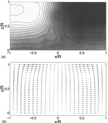
FIG. 3. Mean velocity field in the water experiment: !a" toroidal and !b" poloidal component of the velocity in the meridian plane. The abscissa corresponds to the normalized axial direction with the disks located at x/R #(1, and the ordinate corresponds to the normalized radial direction !with

z/R#0 at the center of the disks". In this measurement, the rotation rate of

meridian plane. Note that axisymmetry and incompressibility are assumed in the extraction of the velocity profile from the measured data.

In addition, at the rotation rates used in the experiment, the von Ka´rma´n flow is strongly turbulent.21–22Velocity fluc-tuations of the order of magnitude of the mean velocity are observed at any given point, as can be seen in Fig. 4 which shows a LDV signal in the water prototype. As a result, care must be taken in interpreting Fig. 3: the flow shown is a time averaged pattern !and not a solution of Navier–Stokes equa-tions" that does not reflect the instantaneous turbulent flow structure.

C. Hydrodynamic measurements in sodium

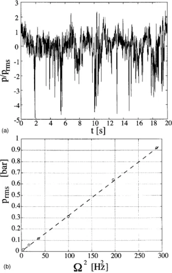
Pressure fluctuations are recorded using a Kistler piezo-electric transducer located in the median plane and mounted flush with the cylindrical wall. Figure 5!a" shows an example of pressure fluctuations in time. The sudden drops are as-cribed to vortex filaments23,24that have been visualized using water seeded with air bubbles;25 their core size has been measured acoustically26and found to be of the order of the Taylor microscale. The rms intensity of the pressure fluctua-tions varies as the square of the rotation rates of the disks, as shown in Fig. 5!b". This yields a measurement of the inten-sity of the rms velocity fluctuations in the flow:24,21

prms-12(urms 2

. !7"

This, in turn, gives an estimate of the intensity of turbulence in the flow, evaluated as the ratio of the rms velocity fluc-tuation to the disk rim speed:

Ku#urms

Urim

#

!

2.R# -0.42, !8"

in good agreement with the water measurements.

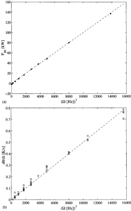
We have also studied the scaling of the power consump-tion of the flow as a funcconsump-tion of the disks’ rotaconsump-tion rate. A dimensional argument in the limit of very large kinetic Rey-nolds numbers yields21

P#KP(R5#3, !9"

where KP is a dimensionless factor that depends on the

ge-ometry of the cell and of the shape of the driving disks. To obtain P, we monitor the current and voltage in the driving motors or we record the temperature drift inside the flow when the external cooling is turned off. Both methods are in good agreement and follow a P/#3 law—cf. Fig. 6. They yield KP#34, in agreement with measurements in the water

prototype with identical impellers where KP#31 is obtained.

III. MAGNETIC INDUCTION A. Measurement scheme

Induction coils are placed with their axis aligned either along the motors rotation axis or perpendicular to it—cf. Fig. 2!a". One can apply to the flow a steady magnetic field B0

with strength in the range 1–20 G. It is distorted by the flow motion so that an induced field b results. We measure the three components of the local magnetic field inside the flow using a temperature calibrated three-dimensional !3D" Hall probe !F.W. Bell". The probe is placed in the axial-vertical plane (xOz) at the same distance from both disks (x#0) and its distance z from the rotation axis is adjustable. The

FIG. 4. Local velocity fluctuations in the water experiment, for a rotation rate equal to 5 Hz, measured from laser Doppler anemometry 5 cm into the flow, at 1/3 of the gap between the disks.

FIG. 5. !a" Time variation of the pressure measured at the flow wall !##17 Hz"; !b" evolution with the disks’ rotation rate of the rms amplitude of the pressure fluctuations. The dashed line corresponds to the quadratic law prms/#2#3.2'10!3%bar/Hz2&.

Hall sensor dynamical range is 65 dB and its time resolution 2.5 ms !in dc mode". The signal is digitized using a 16-bit data acquisition card and stored on a PC.

In the fully turbulent flow under consideration, one ex-pects the magnetic induction to be quite fluctuating. In this section, we first describe the average value of the induced magnetic field and then discuss the statistical characteristics of the fluctuations. One should however bear in mind that averaged and fluctuating components are not independent %cf. Eq. !11"&.

B. Variation of the mean induced field with the applied field

We define the mean magnetic induction, measured at a fixed point in space, as the average over time of the mea-sured data: b ¯#1 T

!

where T is the total time length of the measurement, b is the magnetic induction b#B!B0. Let us begin with the

varia-tion of b with the applied magnetic field B0. At low

ampli-tudes, B0 should not modify the hydrodynamic flow. One

way to quantify its effect is to evaluate the interaction pa-rameter; here N-10!5so that any effect of the applied field is bound to be quite small. When the velocity and magnetic fields are separated into mean and fluctuating parts, the steady state induction equation reads

curl!u¯ÃB0""curl!u¯Ãb¯""curl!u

!

!

1

+,*b¯#0,

!11"

FIG. 6. Variation of the power input in the flow mea-sured !a" from mechanical power delivered the motors !a cubic law best fit yields P/#3_#10!2_%kW/Hz3_{&" and}

!b" from the increase of the temperature inside the flow vessel during one experiment !here, a cubic law fit yields d0/dt/#3_#5'10!5_%K/s/Hz3_&".

where the primes denote the fluctuating part of the fields. If one only considers the effects due to the averaged fields u¯

and b¯, then the equation predicts a linear behavior for b¯(B0).

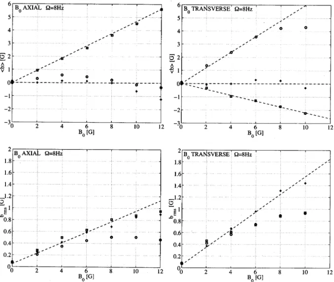
Figure 7 shows the variations of the time averaged mag-netic induction with the external field, applied either along the axis of rotation x or directly perpendicular to it, along y. The 3-D measurement probe is located 10 cm inside the flow, midway between the driving disks. The rotation rate is mod-erate ##8 Hz. As can be observed, the behavior is mostly linear (bi/B0) both for the evolution of the mean magnetic

field components and for their standard deviations. This is what would be expected from Eq. !11" if one assumes that the velocity field does not depend on B. However, for the largest values of the applied field, there are deviations from this simple linear behavior. The magnitude of the induced field !and of its rms intensity" tends to saturate. This effect is not fully understood at present. From Eq. !11", a departure from linearity in b¯(B0) can be caused by a modification of

the velocity field by the magnetic field.

Another observation of the curves shown in Fig. 7 is the anisotropy of the magnetic induction: there are preferred

di-rections for the induced field, depending on the direction of the applied field. For example when B0 is along the axis x,

the main induced component is in the azimuthal direction !i.e., the y direction at the probe location". This effect, al-ready observed in the gallium measurements,27 is attributed to the twisting of the axial magnetic field lines by the differ-ential rotation of the flow—the # effect.1Its strength, mea-sured by the slope of the linear variation of the azimuthal induced field with the magnitude of the applied axial field, yields a definition of an intrinsic magnetic Reynolds number %cf. Eq. !11"&: Rm i -'b ¯ y 'B0 . !12"

Defined in this way, the value of Rm i

varies from 0.5 for a rotation rates of the disks equal to 8 Hz (Rm#20), to 1 at a

rotation rate of 17 Hz (Rm#43). Thus, at high rotation rates,

a toroidal field of strength equal to that of the applied axial field is generated. For comparison, the measurements in the gallium experiment at scale 1/2 gave Rm

i

-0.1.28_{The tenfold} FIG. 7. Mean and standard deviations of the induced field as a function of the applied one, for counter-rotating disks at ##8 Hz (Rm#20). !Left-hand side"

B0is applied along the axis of rotation; !right-hand side" B0perpendicular to the axis of rotation. !!" Axial component bxof the induced field, !"" transverse

component by, !"" vertical component bz. The measurement probe is located near the midplane, 10 cm from the axis of rotation. The dashed lines show a

increase in Rm i

is consistent with changes in the setup char-acteristics: fluid electrical conductivity (,Na-2.2,Ga), fluid

density ((Na-0.16(Ga), size of the experiment (LNa

-2LGa), and power output of the driving motors ( PNa

-7PGa).

When the external field is applied in the transverse di-rection, the largest induced field component is along the axis of rotation, as seen in Fig. 7. At a disk rotation rate of 8 Hz (Rm#20), the magnitude of this induced component is

one-half of the magnitude of the applied field. Again, this ratio reaches 1 at a rotation rate equal to 17 Hz (Rm#43). This

effect is very much increased compared to the gallium ex-periment where the measured induction in the axial direction for a transverse applied field was very small !Rmi -0.025, cf.

Ref. 27, Fig. 5". We believe this increase to be due to our optimization of the sodium flow !propeller design" in which the poloidal to toroidal velocity ratio has been enhanced to a value of 0.8. One important observation is that when the disks are counter-rotated in the opposite direction, the sign of the axially induced component is reversed. Taking into ac-count the symmetries of the mean flow, this means that the axially induced field has opposite directions on each side of a meridian plane (xOy) parallel to the transverse applied field. Altogether, these observations are consistent with an induction mechanism of the$-type due to the swirling mo-tion in the center of the flow. In this large scale mechanism, the toroidal velocity of the swirl motion generates an induced component in the same plane and directly perpendicular to the transverse applied field. This component is then modified by the axial component of the swirl motion to generate an induced current parallel to the applied field, j#!$B0,

where$is proportional to the local helicity 1v•23. The mag-netic field generated is parallel to the rotation axis and changes sign on each side of a meridian plane containing the applied field. Note that it is a two-step mechanism: both poloidal and toroidal velocities contribute.

Finally, we observe that while the mean induction is strongly anisotropic, the intensities of the fluctuations are comparable for all three components of the induced field. However they depend on the direction of the applied field; as seen in Fig. 7, they are stronger when the applied field is in the transverse direction.

C. Evolution with the magnetic Reynolds number

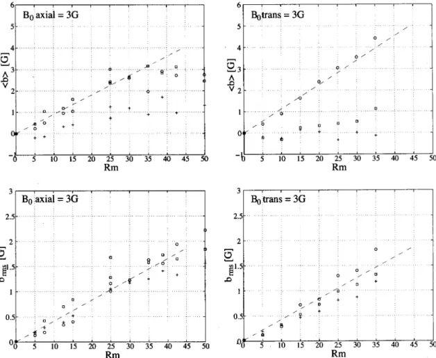
Experiments with a steady externally applied field have been made for rotation frequencies of the impellers between 0 and 20 Hz, corresponding to magnetic Reynolds numbers up to 50. The evolution of the mean and rms values of the three components of the induced field !measured in the me-dian plane" are shown in Fig. 8.

At low disk rotation speed, the behavior is linear: the induced field is proportional to the magnetic Reynolds num-ber. Such a linear behavior is expected at low Rmwhere the

dominant induction mechanism is due to the stretching of the magnetic field lines by the mean flow velocity gradients. In this ‘‘quasistatic’’ approximation, the induction equation re-duces to

curl!u¯ÃB0""

1

+,*b¯#0. !13"

As a result of our optimization procedure, the poloidal and toroidal velocities contribute almost equally to the induction. This can be observed in Fig. 8!a": the azimuthal !y-component" and axial !x-!y-component" induced fields are of the same order (b¯y-0.7b¯x). They are due, respectively, to

the toroidal and poloidal part of the mean flow velocity, as can be inferred from symmetry considerations.

When the external field is along the rotation axis—Fig. 8!a", the main effect is the generation of a toroidal induced component via the # effect. An induced component along the axis is also generated, as a linear mechanism, from the stretching by the axial velocity gradients—note that uaxial

changes direction in the median plane (yOz). The third !ra-dial" component is almost null, in agreement with the sym-metries of the mean flow.

When the external field is applied in the transverse di-rection, the induction in the median plane is dominant in the axial direction, at all rotation frequencies. In this case, the contribution of the linear induction by the mean flow van-ishes. Indeed, along the axis, Eq. !13" reduces to

1

+,*b¯x#!B0 '¯u_x

'y . !14"

In the median plane the axial velocity of the mean flow is zero, and so are its derivatives along any direction in that plane. The axial induction must thus originate from other sources than such a local induction mechanism. As pointed out previously, a possible source of induction is the helicity in the central part of the flow where the poloidal and toroidal velocity component can produce a macroscopic $ effect. This would be consistent with the fact that, like the helicity, the axial induced field is reversed if the disks are rotated in opposite directions. However, in that case, we would expect the magnitude of the axial induced field to vary quadratically with the rotation rate of the discs. This is not observed in Fig. 8!b".

At higher rotation rates, we note a change in behavior: despite the increase in the disks’ rotation rate, the amplitude of the induced field seems to saturate. Several mechanisms can be responsible for this behavior. First, but not very likely, the increased induced field may become large enough to modify the velocity gradients in the flow or, as discussed previously, the correlations between the fluctuations of mag-netic and velocity fields. The second and more plausible ef-fect is that, as Rm increases, the induction becomes

nonlin-ear: the velocity distorts the applied field B0 to generate an

induced field b1, which in turn can be distorted to generate

b2, and so on. The expulsion of magnetic field lines by a

coherent vortex28or the self-generation of a dynamo8 –10are examples of the piling of such effects leading to a divergence of the induced field.

Note that for these large Rmexperiments, the magnitude

of the induced field overcomes the applied field. In Figs. 8!a" and 8!b", b¯ reaches almost 6 G, twice the magnitude of the

Finally, we observe that the induction fluctuations are isotropic at all rotation rates: all three components of the induced field have comparable rms fluctuation level, defined as the ratio of the standard deviation to the mean, ranging from 20% to 50% of the mean. As the magnetic Reynolds number increases, the intensity of the fluctuation becomes independent of the direction of the applied field.

D. Fluctuations of the magnetic induction 1. Overview

The data shown in the previous section are averaged over long periods of time. Due to the large value of the kinetic Reynolds number, turbulence is quite developed, with rms velocity fluctuations as high as 42% of the mean veloc-ity !cf. Sec. II". As noted in Figs. 7 and 8, all magnetic field components also display rms fluctuations of the same order of magnitude. This section is devoted to the analysis of these induction fluctuations.

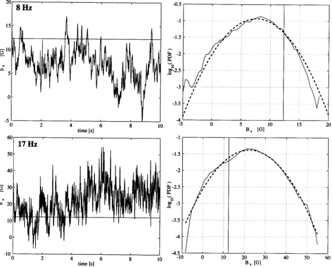
Figure 9 actually gives two examples of the time varia-tions of the axially induced field for a transverse B0

#12.3 G, at rotation rates equal to ##8 Hz and ##17 Hz. At ##8 Hz (Rm#20) the induced field fluctuates about a

value that is less than the amplitude of the applied field. On the contrary, at ##17 Hz (Rm#43) it fluctuates about a

value that is larger than that of the applied field. In both cases, we observe that the fluctuations are distributed over a Gaussian statistics whose variance varies as shown in Figs. 8!c" and 8!d". This is verified for all magnetic field compo-nents and at all the rotation rates covered in this set of experiments—all the probability density functions of the in-duced magnetic field, and normalized to its standard devia-tion, collapse onto the same Gaussian distribution.

Another specific feature of induction fluctuations is the presence of two ranges of time scales in the time signal %Fig. 9!a"&: small-amplitude fast fluctuations are superimposed over large-amplitude slow variations. As shown later in this section, the fast fluctuations can be described by a Kolmog-orov approach of the turbulent stretching of the magnetic field lines. The slow dynamics !time scales of the order of the disks’ rotation frequency and lower" plays a more impor-tant role in the fluctuations of induction. It is responsible for the overall amplitude of the rms fluctuation level: the rms amplitude of the signal is nearly unchanged if it is low-pass filtered below #—at all rotation rates, the contribution of the modes at frequencies higher than # is equal to 10% of the total rms intensity level. Such long time scales can be asso-ciated with ‘‘global’’ fluctuations of the mean flow which are known to exist in this geometry.29,22That is, if one defines a

FIG. 8. Mean and standard deviations of the induced field as a function of the magnetic Reynolds number of the flow. !Left-hand side" Axial B0#3 G, and

!right-hand side" transverse B0#3 G. !!" Axial component bx of the induced field, !"" transverse component by, !"" vertical component bz. The

‘‘mean’’ flow as the average flow pattern over a time scale of the order of the forcing time !e.g., the period of rotation of the disks", then one observes that this pattern varies in time. The geometry of the flow thus fluctuates about a configura-tion such as shown in Fig. 3 and successive realizaconfigura-tions may lead to varying intensity induction. These variations are de-tected by the local magnetic probe because the diffusive time scale across the flow size is long. Dimensional analysis yields4diff#+0,R2-0.5 s, while pulse-decay measurements

in the spirit of Peffley et al.17 yield 4diff-0.15 s. For

com-parison, the advection time of any flow or magnetic field structure past the measurement probe is much shorter: 4adv

-dprobe/urms-1 ms.

2. Correlations

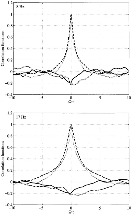
The slow-scale/large-scale dynamics of the magnetic field is further confirmed by correlation functions analysis. In Fig. 10, we consider the induction in the case of an applied field transverse to the rotation axis. The autocorrelation of the magnetic field component in the axial direction !dashed curves" decreases with a characteristic time of order #!1

and is zero for time lags larger than about 10 #!1. This is also the case for the autocorrelation function of the pressure measured at the flow wall !dotted line in Fig. 10". The in-duced field components are also cross-correlated with iden-tical characteristic times.

The most significant evidence of the large scale nature of the magnetic field dynamics is the existence of a correlation

5p!Bbetween the pressure measured at the flow wall and the

induced magnetic field measured internally by the Hall probe. Indeed, as shown in Fig. 10 !solid lines", we observe

5p!b_x-!0.2 at t#0. !15"

This is a quite significant figure considering that the mea-surements are made at points located some 15 cm away in a flow with a Reynolds number larger than 106. The charac-teristic damping time of the pressure-induction cross-correlation is again of the order of the flow forcing time scale #!1_{; decorrelation is achieved for time lags longer than}

10 #!1. Recalling that the fluctuation in time of the pressure at a flow wall are related to the fluctuations in the distribu-tion of the velocity gradients !the pressure obeys the Poisson

FIG. 9. Time variation !left-hand side", and corresponding probability density function !right-hand side", for the axial component of the induced field for a transverse applied field B0#12.3 G. !Upper" Disks’ rotation rate ##8 Hz (Rm#20); the induced field has a magnitude of 7.6 G, with a standard deviation

equal to 3.4 G; !lower" disks’ rotation rate ##17 Hz (Rm#43); the induced field has a magnitude of 22.2 G, with a standard deviation equal to 9.6 G. The

dashed curve on the right-hand side is the Gaussian PDF for a variable having the same mean and variance as the data. The horizontal !left" and vertical !right" lines mark the magnitude of the applied field.

equation * p#!('iuj'jui", the pressure-induction

correla-tion at large time shows the slow dynamics of the magnetic field to be linked to corresponding slow changes in the flow topology. These correlations of the fluctuating parts of the magnetic and velocity fields play a major role in the dynam-ics of induction.

3. Spectra and increments

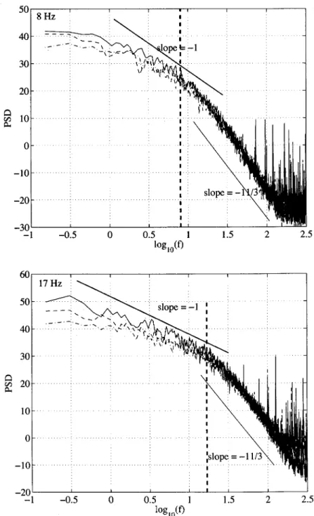
The time spectra for each component of the induced field are shown in Fig. 11. The curves are very similar for all three components of the induced field. Three frequency regimes are clearly identified.

a. High frequency range. For frequencies higher than

#, the spectra decay algebraically with a slope close to !11/3. This regime corresponds to the action of the turbulent velocity fluctuations, in agreement with Kolmogorov K41

phenomenology,30 provided a Taylor hypothesis can be ap-plied to the fast magnetic field fluctuations. At low Rm, this

spectral behavior results directly from Eq. !13" which yields

b2

!!k"/k!2_u!!k"-k2 !11/3 _!16"

in Fourier space, if a traditional u2_(k)-k!5/3 _Kolmogorov

spectrum is assumed for the velocity field at small scales. This high-frequency scaling behavior was observed in our previous gallium experiment.27 We find here that it is also valid at the significantly higher magnetic Reynolds numbers reached in the sodium setup. It is consistent with other stud-ies in sodium flows31,17and with numerical studies of MHD turbulence at high Rm. In addition, some simulations32have

shown that the relationship b˜2_(k)/k!2˜ (k) between kinetic_u2 FIG. 10. Correlations in the case of a transverse applied field. The measurement probe is located near the mid-plane, 10 cm from the axis of rotation. The pressure probe is mounted flush with the inner wall, at a distance d#15 cm from the magnetic probe. !Dashed line": au-tocorrelation function of the axial component of the in-duced field5(bx!bx); !dotted line": autocorrelation of

the pressure at the wall5(p!p); !dash-dotted line": cross correlation of the axial and transverse induced fields5(bx!by); !solid line": cross correlation between

the pressure and the axially induced field 5(p!bx).

Upper panel: disks’ rotation rate at 8 Hz (Rm#20) and

and magnetic energy subsists for a dynamo-generated mag-netic field although both spectra are steeper due to the effect of the Lorentz force.33,34

b. Intermediate frequency range. For frequencies

be-tween #/10 and # we observe another power law behavior with an exponent close to !1. This power law regime

b

˜2_{( f )/ f}!1_{was not readily observed in the gallium setup. A}

similar regime has been found in the Maryland experiment from measurements made outside the flow volume but with an exponent close to to !5/3.17,18The same spectral regime has been reported in the Karlsruhe experiment for the mag-netic field fluctuations above dynamo threshold. We also note that this type of spectral behavior is reminiscent of the low frequency part of the velocity spectrum for turbulent flows with strong shear, in which context it is attributed to the

domination of the velocity gradient tensor by a large scale shearing contribution: for time intervals larger than some characteristic shearing time, vorticity stretching has reached its maximum value. It is actually instructing to analyze this 1/f behavior in the time domain rather than in the frequency domain, i.e., via the time increments of the induction:

6b!4"#b!t"4"!b!t". !17" The 1/f scaling domain could be explained by the saturation of the increments for times larger than #!1. Indeed,6b(4) -40_{would yield a b˜}2_{( f )/ f}!1_{behavior. This hypothesis can}

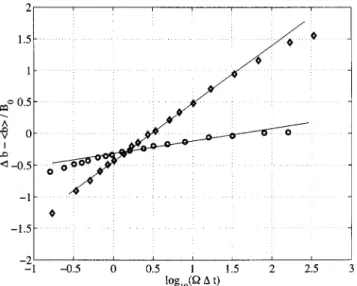
be tested by computing the peak to peak value of the mag-netic induction max(b)!min(b) and averaging this quantity over varying *t time intervals. As shown in Fig. 12, we observe a logarithmic behavior

FIG. 11. Power spectrum of the three components of the magnetic induction; x component: black line, y component: dashed line; z component: dash-dotted line. The applied field is transverse, with a magnitude of 12.3 G. The thick dashed line indicates the forcing fre-quency, i.e., the impellers rotation rate #. The measure-ment probe is located near the midplane, 10 cm from the axis of rotation. Upper panel: disks’ rotation rate at ##8 Hz (Rm#20) and lower panel: disks’ rotation rate

1

3

!18" for all time intervals larger than *t-#!1. This time behav-ior is consistent with the 1/f spectral variation, since a loga-rithmic law can be viewed as the limit of an algebraic func-tional form with a vanishing exponent.

c. Low frequency part. For frequencies lower than about #/10, the spectral content is flat. This behavior is char-acteristic of uncorrelated magnetic fluctuations. It is consis-tent with previous observations of velocity fluctuations in this type of flow becoming uncorrelated for times larger than 20–50 disks rotation periods.29,22

Altogether, our observations show that, in regards to the fluctuations of induction, the turbulent velocity fluctuations in the inertial range play a minor role. They occur at high frequency and display a very steep decay so that their con-tribution to brmsis quite small. The main effect is due to slow

variations with characteristic times between 1 and 10 periods of rotation of the driving disks. We attribute them to slow changes of the flow topology. As the global structure of the velocity gradients vary, so does the induction at all points. We find that some geometries of the swirling flow are very efficient magnetic field amplifiers: for certain realizations, the peak induced field can be ten times larger than the ap-plied field.

IV. CONCLUDING REMARKS

Using a specific sodium device, we have studied the magnetic field dynamics in a von Ka´rma´n flow at magnetic Reynolds numbers in the range 5–50. High speed runs up to

Rm#65 have also been performed. Due to the fast

tempera-ture increase !"1 K s!1_{", these runs were short and produced}

few dispersed data. A cooling system is under construction in order to produce high quality data at such high Reynolds numbers.

Our internal measurement of the induced 3D magnetic field in the presence of an externally applied field shows strong and anisotropic induction mechanisms. They are re-lated to the two main features of the flow geometry: the differential rotation, which drives an # effect, and the helic-ity, which can produce a macroscopic$effect. These are two major ingredients of dynamo action, although self-generation has not been reached in this experiment so far. Another very important feature of the induction is its very high level of global fluctuations in time. As explained, this effect is related to the flow nonstationarity. It has some strong implication for the observation of dynamo action in unconstrained flows. Indeed, even if some particular flow topology would be fa-vorable to strong magnetic amplification, they may not last long enough, or maintain a sufficient coherence in time, for a self-sustained magnetic amplification to take place: we have observed flow global variations to occur with characteristic times of the order of the magnetic diffusive time. Further experimental campaigns are under way to clarify this prob-lem.

ACKNOWLEDGMENTS

The authors gratefully acknowledge the financial support of the French institutions: Commissariat a` l’E´nergie Atom-ique, Ministe`re de la Recherche and Centre National de Re-cherche Scientifique. J.B. was supported by post-doctoral Grant No. PB98-0208 from Ministerio de Educacio´n y Cien-cias !Spain" while at CEA-Saclay.

1_{H. K. Moffatt, Magnetic Field Generation in Electrically Conducting}

Flu-ids !Cambridge University Press, Cambridge, 1978".

2

R. Moreau, Magnetohydrodynamics !Kluwer, Dordrecht, 1990".

3_{A. Alemany, R. Moreau, L. Sulem, and U. Frisch, ‘‘Influence of an}

exter-nal magnetic field on homogeneous MHD turbulence,’’ J. Mec. 18, 278 !1979".

4_{S. Fauve, C. Laroche, and A. Libchaber, ‘‘Effect of a horizontal magnetic}

field on convective instabilities in mercury,’’ J. Phys. !France" Lett. 42, L455 !1981"; ‘‘Horizontal magnetic and the oscillatory instability onset,’’

45, L101 !1984".

5_{R. Moreau and J. Sommeria, ‘‘Why, how and when MHD turbulence}

becomes two-dimensional,’’ J. Fluid Mech. 118, 507 !1982".

6_{J. Larmor, ‘‘How could a rotating body such as the sun become a}

mag-net?’’ Rep. Brit. Assoc. Adv. Sci., 159 !1919".

7_{A. Gailitis, O. Lielausis, S. Dement’ev, E. Placatis, A. Cifersons, G.}

Ger-beth, T. Gundrum, F. Stefani, M. Chrsiten, H. Ha¨nel, and G. Will, ‘‘De-tection of a flow induced magnetic field eigenmode in the Riga dynamo facility,’’ Phys. Rev. Lett. 84, 4365 !2000".

8_{A. Gailitis, O. Lielausis, S. Dement’ev, E. Placatis, A. Cifersons, G.}

Ger-beth, T. Gundrum, F. Stefani, M. Chrsiten, H. Ha¨nel, and G. Will, ‘‘Mag-netic field saturation in the Riga dynamo experiment,’’ Phys. Rev. Lett. 86, 3024 !2001".

9_{Yu. B. Ponomarenko, ‘‘Theory of the hydromagnetic generator,’’ J. Appl.}

Mech. Tech. Phys. 6, 755 !1973".

10_{R. Stieglitz and U. Mu¨ller, ‘‘Can the Earth’s magnetic field be simulated in}

the laboratory?’’ Naturwissenschaften 87, 381 !2000".

11_{R. Stieglitz and U. Mu¨ller, ‘‘Experimental demonstration of a}

homoge-neous two-scale dynamo,’’ Phys. Fluids 13, 561 !2001".

12_{G. O. Roberts, ‘‘Kinematic dynamo models,’’ Philos. Trans. R. Soc.}

Lon-don, Ser. A 271, 411 !1972".

13_{N. L. Dudley and R. W. James, ‘‘Time-dependent kinematic dynamos with}

stationary flows,’’ Proc. R. Soc. London, Ser. A 425, 407 !1989".

14_{J. Le´orat, private communication at the 2nd Pamir Conference, Aussois}

!France", September 1998.

15

L. Marie´, J. Burguete, A. Chiffaudel, F. Daviaud, D. Ericher, C. Gasquet, F. Pe´tre´lis, S. Fauve, M. Bourgoin, M. Moulin, P. Odier, J.-F. Pinton, A.

FIG. 12. Evolution of the peak to peak value of the magnitude of the induced magnetic field%6b(*t)#max(b)!min(b)& as the interval *t over which it is calculated increases. Two experiments are shown !!": disks rotating at 8 Hz (Rm#20) and !"": disks’ rotating at 17 Hz (Rm#43). The

Guigon, J.-B. Luciani, F. Namer, and J. Le´orat, ‘‘MHD in von Ka´rma´n swirling flows,’’ in Ref. 18.

16_{C. Nore, M.-E. Brachet, H. Politano, and A. Pouquet, ‘‘Dynamo action in}

the Taylor–Green vortex near threshold,’’ Phys. Plasmas 4, 1 !1997".

17

N. L. Peffley, A. B. Cawthrone, and D. P. Lathrop, ‘‘Toward a self-generating magnetic dynamo: The role of turbulence,’’ Phys. Rev. E 61, 5287 !2000".

18_{W. L. Shew, D. R. Sisan, and D. P. Lathrop, ‘‘Hunting for dynamos: Eight}

different liquid sodium flows,’’ in Dynamo and Dynamics, A Mathematical

Challenge, Proceedings of the NATO Advanced Research Workshop,

Carge`se, France, 21–26 August 2000. NATO Science Series II, Vol. 26, edited by P. Chossat, D. Armbruster, and I. Oprea !Kluwer Academic, Dordrecht, 2001".

19_{D. Sweet, E. Ott, J. M. Finn, T. M. Antonsen, Jr., and D. P. Lathrop,}

‘‘Blowout bifurcations and the onset of magnetic activity in turbulent dy-namos,’’ Phys. Rev. E 63, 066211 !2001"; D. Sweet, E. Ott, T. M. Anton-sen, Jr., D. P. Lathrop, and J. M. Finn, ‘‘Blowout bifurcations and the onset of magnetic dynamo action,’’ Phys. Plasmas 8, 1944 !2001".

20_{P. J. Zandbergen and D. Dijkstra, ‘‘von Ka´rma´n swirling flows,’’ Annu.}

Rev. Fluid Mech. 19, 465 !1987".

21_{N. Mordant, J.-F. Pinton, and F. Chilla`, ‘‘Characterization of turbulence in}

a closed flow,’’ J. Phys. II 7, 1 !1997".

22_{J.-F. Pinton and R. Labbe´, ‘‘Correction to Taylor hypothesis in swirling}

flows,’’ J. Phys. II 4, 1461 !1994".

23_{O. Cadot, S. Douady, and Y. Couder, ‘‘Characterization of the}

low-pressure filaments in a three-dimensional turbulent shear flow,’’ Phys. Flu-ids 7, 630 !1995".

24

S. Fauve, C. Laroche, and B. Castaing, ‘‘Pressure fluctuations in swirling turbulent flows,’’ J. Phys. II 3, 271 !1993".

25_{S. Douady, Y. Couder, and M.-E. Brachet, ‘‘Direct observation of intense}

vorticity filaments in turbulence,’’ Phys. Rev. Lett. 67, 983 !1991".

26_{B. Dernoncourt, J.-F. Pinton, and S. Fauve, ‘‘Study of vorticity filaments}

using ultrasound scattering in turbulent swirling flows,’’ Physica D 117, 181 !1998".

27_{P. Odier, J.-F. Pinton, and S. Fauve, ‘‘Advection of a magnetic field by a}

turbulent swirling flow,’’ Phys. Rev. E 58, 7397 !1998".

28_{A. Martin, P. Odier, J.-F. Pinton, and S. Fauve, ‘‘Magnetic permeability of}

a diphasic flow, made of liquid gallium and iron beads,’’ Eur. Phys. J. B

18, 337 !2000".

29_{L. Marie´ et al., Proceedings of the Sixth European Chaos Conference,}

Potsdam, Germany, 22–26 July 2001, edited by S. Boccaletti, L. Peccora,

and J. Kurths !American Institute of Physics, Melville, NY, 2002".

30_{H. K. Moffatt, ‘‘The amplification of a weak applied magnetic field by}

turbulence in fluids of moderate conductivity,’’ J. Fluid Mech. 11, 625 !1961".

31_{A. Alemany, P. Marty, F. Plunian, and J. Soto, ‘‘Experimental investigation}

of dynamo effect in the secondary pumps of the fast breeder reactor Su-perphenix,’’ J. Fluid Mech. 403, 263 !2000".

32_{U. Frisch, A. Pouquet, J. Le´orat, and A. Mazure, ‘‘Possibility of an inverse}

cascade of magnetic helicity in magnetohydrodynamic turbulence,’’ J. Fluid Mech. 68, 769 !1975".

33_{G. S. Golitsyn, ‘‘Fluctuation of the magnertic field and current density in}

a turbulent flow of a weakly conducting fluid,’’ Sov. Phys. Dokl. 5, 536 !1960".

34_{F. Pe´tre´lis, L. Marie´, M. Bourgoin, A. Chiffaudel, F. Daviaud, S. Fauve, P.}

Odier, and J.-F. Pinton, ‘‘Large scale alpha-effect in a turbulent swirling flow,’’ arXiv:physics/0205019 !2002".