Transition to turbulence via spatiotemporal intermittency in one-dimensional Rayleigh-Bénard convection

HAL Id: cea-01374027

https://hal-cea.archives-ouvertes.fr/cea-01374027

Submitted on 29 Sep 2016

HAL is a multi-disciplinary open access

archive for the deposit and dissemination of

sci-entific research documents, whether they are

pub-lished or not. The documents may come from

teaching and research institutions in France or

abroad, or from public or private research centers.

L’archive ouverte pluridisciplinaire HAL, est

destinée au dépôt et à la diffusion de documents

scientifiques de niveau recherche, publiés ou non,

émanant des établissements d’enseignement et de

recherche français ou étrangers, des laboratoires

publics ou privés.

intermittency in one-dimensional Rayleigh-Bénard

convection

F. Daviaud, M. Bonetti, M. Dubois

To cite this version:

F. Daviaud, M. Bonetti, M. Dubois. Transition to turbulence via spatiotemporal intermittency in

one-dimensional Rayleigh-Bénard convection. Physical Review A, American Physical Society, 1990,

42 (6), pp.3388 - 3399. �10.1103/PhysRevA.42.3388�. �cea-01374027�

Transition

to turbulence

via spatiotemporal

intermittency

in one-dimensional

Rayleigh-Benard

convection

F.

Daviaud,

M.

Bonetti, and

M.

Dubois

Service dePhysique du Solide et de Resonance Magnetique, Centre d'Etudes Nucleaires de Saclay, F-9119IGifsur Yve-tte CEDEX,Fmnce

(Received 7 March 1990)

Rayleigh-Benard convection is studied in quasi-one-dimensional geometries. Fixed and periodic boundary conditions are imposed using a rectangular and an annular cell, respectively. The desta-bilization process ofthe homogeneous convective pattern isstudied for increasing Rayleigh number

A.

Thefirst time-dependent behaviors aregiven by the appearance ofcoupled oscillators. At larger

A values, the spatial breakdown appears through the propagation ofspatial defects, which appear

to be solitary waves. This spatiotemporal destabilization is followed at higher %by a spatiotem-poral intermittent regime, which corresponds to adramatic decrease ofthe spatial coherence and to

amixing ofturbulent patches within laminar domains. This last regime isstudied within the frame

ofphase transitions. The statistical analysis evidences a second-order phase transition at least inthe rectangular geometry (fixed boundary conditions), while this transition looks imperfect in the

annu-lar geometry (periodic boundary conditions). Nevertheless, the essential qualitative features shown by theoretical and numerical models are observed in both geometries. Comparison with a simple

model ofdirected percolation shows that the imperfect nature ofthe transition in the annulus could

be the consequence ofsome mechanism ofself-generation ofthe turbulent domains. This

mecha-nism is, however, unknown but isprobably related tothe influence ofthe boundaries.

I.

INTRODUCTION

The evolution towards turbulent states

of

one-dimensional

(ID)

hydrodynamical systems has recently

received much interest. In fact, these systems are

classified between the highly confined systems where

deterministic chaotic dynamics might be observed and

the extended systems in which developed turbulence

gen-erally takes place. Theoretical studies on these systems,

which depend mainly on one space variable, have shown

that a steady periodic cellular state may destabilize and

become turbulent when acontrol parameter is varied. In

this context, numerical simulations

of

phase equations,

such as those derived from the Kuramoto-Sivashinsky

equation, ' coupled map lattices, ' _{and cellular}

auto-mata show that turbulence can be reached via

spatiotem-poral intermittency

(STI).

This

STI

regime corresponds

to a mixture

of

organized and turbulent domains which

exchange themselves in space and time.

In very recent years, experiments were done on 1D

sys-tems in which the basic state is spatially periodic. In this

frame, Rayleigh-Benard convection was studied in cells

with narrow gaps (one horizontal dimension is much

larger than the other) where only one space variable is

in-volved. Specific spatial and dynamical properties were

observed, as well as

STI

(Ref. 6) at high values

of

the

Rayleigh number. Statistical analysis

of

STI

regimes,

performed under more adequate experimental

condi-tions, ' _has

given results similar

to

those

of

numencal

simulations. Nevertheless, the nature

of

the transition,

which could be reminiscent

of

a direct percolation

pro-cess, left some questions unanswered.

In order to get a deeper understanding

of

the

dynami-cal regimes involved in this transition toturbulence

—

via

STI

—

in 1Dsystems, we report detailed experimental

re-sults

of

convection in annular (periodic boundary

condi-tions) and in rectangular (fixed boundary conditions)

geometries. The two flows exhibit

STI

above a given

Rayleigh number, but whereas the transition is almost

perfect in the rectangular case, it turns out tobe imperfect

in the annulus, probably owing

to

the existence

of

local

instabilities preceding the sustained

STI

regime.

In the following, we first describe the experimental

set-up and discuss the conditions relevant to the experiments

(Sec.

II).

In

Sec.

III

we present the regimes leading to

STI

and the existence

of

solitary waves. The statistical

properties

of

STI

in both geometries are discussed in

Sec.

IV.

The use

of

a spatial criterion

to

discriminate laminar

domains (LD's) from turbulent domains (TD's) allows us

to perform a detailed statistical analysis in the case

of

the

annular (Sec. IVA) and rectangular (Sec. IV B)

geometries. In

Sec.

V we show numerical results

of

directed percolation and compare them with

experimen-tal data. Finally, in

Sec.

VI, the convective regimes in

both geometries and the nature

of

the transition to

STI

are discussed.

II.

EXPERIMENTAL CONDITIONS

Experiments were performed both in annular and

rec-tangular cells filled with silicon oil

of

Prandtl number

P=7.

Both geometries had vertical walls in Plexiglass.

The annular and rectangular cells had sapphire and

copper horizontal plates, respectively. In order to get a

quasi-1D geometry, ' the annular cell had a circumferen-tial aspect ratio

I,

=2vrr

/d

=35

and a radial aspect

ra-tio

I

„=Dr/d =0.

29 where

r,

b,r, and d are the mean

radius, the radial gap, and the cell depth (d

=7

mm for

the two cells). In the rectangular cell the longitudinal

as-pect ratio was

I

„=L„/d

=25.

7 and the transverse

as-pect ratio was

I

=L

/d

=0.

43.

In the two sets

of

ex-periments the temperature difference across the fluid

lay-er was kept constant to within

0.

01

K

by means

of

circu-lating thermal regulated

~ater.

The convective structures were visualized by

shadow-graphic imaging. A parallel light beam crossed vertically

the annular cell through the horizontal sapphire plates,

while in the rectangular cell, the beam was shone

perpen-dicularly through the horizontal longest side

L

. In this

way, the beam deflection was integrated along the cell

depth (circular cell) and along the smallest horizontal

di-mension (rectangular cell). One had therefore the top

view

of

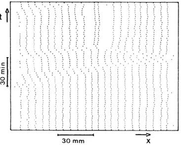
the convective pattern in the circular geometry

and the front view in the rectangular one (seeFig. 1).

The temporal evolution

of

the annular roll pattern was

recorded using either a circumferentially moving

photo-diode positioned at the place

of

the shadowgraphic image

or a video camera recording system. With the former

technique, the annular convective structure was

azimu-thally scanned every second over 260spatial points giving

near the onset

of STI

a spatial resolution

of

—

6

points/wavelength. The video technique was used in

both geometries and, as the convective dynamics is

quasi-1D, the shadowgraphic image was digitized along a

circle

of

approximately 1200 pixels (annular cell) or an

horizontal line

of

512 pixels (rectangular cell), giving a

spatial resolution

of

-30

pixels and

—

16 pixels per

wavelength, respectively. The circle and line were

ap-propriately selected in order to get a representative

skeleton

of

the convective pattern, without losing too

much information on the flow dynamics. The acquisition

frequency could be increased up to 5 circles/sec and 20

lines/sec for the annulus and rectangle, respectively.

In both geometries the time lapse between each new

line acquisition was set according towhich dynamics,

i.

e._,

a short or along time evolution, was studied.

For

exam-ple, when we analyzed the spatiotemporal intermittency,

we looked particularly at the long time evolution

of

the

roll pattern. In the rectangular cell, up to 1900lines were

recorded with a time interval generally set to 3sec;in the

annular cell, time series up to 2000 sec were recorded.

The total acquisition time is to be compared to a charac-teristic time, namely, the basic period To

of

the rolls os-cillators. As To—-1 and 2 sec in the rectangular and

an-nular cells, respectively, this yields a total acquisition

time

of

about 6000 and 1000 basic oscillations

of

the

rolls.

After each temperature increase, dynamical

equilibri-um must be reached. In both experiments, we waited as

long as 24 h up to 48 h before each new data acquisition.

As a matter

of

fact, these delays revealed themselves

sufficient to obtain a new equilibrium dynamical regime.

The comparison with the phase diffusion time

=

_L,

_/D

~~ cannot easily be done since

D

~~

isnot known for

these narrow geometries and high Rayleigh numbers.

Nevertheless, taking _D~~

=2.

2X10

cm sec ' as

calcu-lated (and measured) near the convective onset,

"

these

delays are considered sufficient (rD

=2

and 3days for the

rectangular and the annular geometries, respectively).

III.

FLOW EVOLUTION

BELOWTHESPATIOTEMPORAL

INTERMITTENT REGIME

Spatial and dynamical properties specific to the narrow

channels, (i.e.,

I,

(0.

5), have been already reported

else-where. ' They are summarized as follows. When

R

exceeds a critical value

_%,

=f

(I

~), perfect stationary

patterns are observed with the roll's axis perpendicular to

the longest side

of

the container. An increase

of

A

in-duces generally the appearance

of

new rolls, making the

wavelength A,

of

the pattern much smaller than the one

observed in large containers. ' Wavelengths down to 2L

can be obtained. The value

of

k depends on the Rayleigh

number and on the thermal history. Near the onset

of

STI

and in a reproducible manner, 30 Q,

O=0. 43k,

with

A,

,

=2d)

and 40

(10=0.

44k.

,

) wavelengths Ao are present

in the rectangular channel and the annular channel,

re-spectively. In the annular geometry, at lower

%

values, a

stable spatial inhomogeneity

of

the local wavelength is

generally observed and up tonow, no clear explanation

of

this phenomenon has been given.

Above a given e value

[@=A/A,

(1"~)

—

I]

which

de-pends on the transverse aspect ratio

I

and on the

present wavelength, the pattern becomes time dependent

with the appearance

of

thermal oscillators (domain

la-beled by Din Fig. 2).

In the rectangular channel, at

a=310,

hot plumes

ap-FIG.

1. Shadowgraphic image of1DRayleigh-Benard convection in a rectangular container with I_~

=0.

3at @=45.Bright and

200 400 pre STI STI t I I I I I I I 600 (b) 200 STI 0 t I I I I I 310 g' 4pp I I 'I I I I I I 600

FIG.

2. Phase diagram ofthe convective state as a function ofein the annular cell (a) and inthe rectangular channel (b). S stands for astationary pattern, Dfor a time and/or spatial os-cillating pattern, STI for spatiotemporal intermittency, and T for a complete disorganized and turbulent pattern.

I I I I h I I I I I I I I I I I I I I I I I I I I I I I I I I I I I I I I I I I I I I I I I I I I I I I I I I I I I 1 I 1 I I I I I I I I I I I I I I I I I I I I I t I I I I 1 I 1 I I I I I 1 I I I 1 t I I I I I I I I I I I I I I I I I I I I I I I I I I I I I I I I I I I I I I I I I I I I I I I I I 1 I I I I I I I I I I I I I I I I I I I I t I I I I I I I I I I I I I I I I I I I I I I I I I I I I I I I I I I I I I I I I I I I I I I I I I I I I I I I I I I I I I I I I I I I I t I I I I I I I I I I I I I I I I I I I I I I I I I I I I I I I I I I I I I I I I I I I I I I I I I I I I I I I I I I I I I I I I I I I I I I I I I I I I I I I I I I I t I I I I I I I I I I I I I I I I I I I I I I I I I I I I I I t I I I I I I I I I I I I I I I I I I I I I I I I I I I t I I I I I I I I I I I I I I I I I I I I I I I I I I I I 1 I I I I I I I I I I I I I I I I t I I I I I I I I I I I I I I I I I I I I I I I I I I t I I I I I I I I I I I I I II I t I I I I I I I I I I I I I I I I I I I I I I I I I I I I ~ I I I t I I I I I I I I I I I I I I I I I I I I I I I I I I I I I I I I I I I I I I I I I I I I I I I I I I I I I I I I I I I I I I I I I I I I I I I I I I I I I I I I I I I I I I I I I I I I I I I I I I I I I I I I I I t I I I I I I I I I I I I I I I I I I 1 I 1 I I I I I 1 I I I I I I I I I I I I t I 1 I 1 I t I I I I I I I 1 I I I 1 I I 1 I 1 t I 1 I I 1 I I I I I I I I I I I I I I I I I I I 1 t I I I t I I I I I I I I I I I I I I I I I I I I I I I I I I t 1 I I I I I I I I I I I I I I I I I I I I I I I I I I I I I I I I I I I I I I I I I I I I I I I I I I I I I I I I I I I I I I I I t I I I I I I I I I I I I I I I I I I I I I I t I I I I I I I I I I I I I I I I I I I I I I I I I I I I I I I I I 1 I I I I I I I I I I I I I I I I I I I I I I I t I I I I I 1 I I I I I I I I I I I I I I I t I I I I I I I 1 I I I I I I I I I t I I I I I I I I I I I I I I I I I I I I I I I I I I I

30

mm X

pear periodically in a pattern with a wavelength

A,

=0.

45k,

The system is at first monoperiodic,

i.

e._, all

the plumes have the same frequency everywhere and the

convective rolls are similar

to

a chain

of

coupled

oscilla-tors.

In the annular cell, collective oscillations are observed

for

e

&_{200and are related to a mechanism}

_of

_{Uacillations,}

as it has been described in

Ref.

12. We recall that these

vacillations, which correspond to a periodic

displace-ment, in phase opposition,

of

the ascending and

descend-ing streams around their mean position, are specific to

the narrow channels with

_Iy

0

40 When the Rayleigh

number is further increased, the collective periodic

be-havior may become chaotic with properties similar to

those

of

a pure dynamical system, while the spatial

prop-erties remain unchanged. Still in the annulus, a small

evolution

of

the pattern, probably induced by aslow and

anonhomogeneous drift

of

the phase

of

the rolls can also

be observed, but globally the spatial features

of

the

pat-tern remain unchanged with a wavelength dispersion as

already mentioned.

At a larger value

of

e, new events leading to aspatial

symmetry breaking appear. These events were observed

in a stationary pattern present in a rectangular channel

between horizontal glass plates. ' The behavior is the

fo11owing: in an otherwise perfect pattern, a local

desta-bilization produces a wavelength larger than its

neigh-bors. This defect, which extends over two or three

wave-lengths, propagates along the pattern and can be reflected

at the lateral walls while keeping its topological aspect

(Fig. 3). Therefore it looks like a solitary wave. These

waves, which have been further observed within the

ex-perimental conditions

of

the results reported here, are

difficult

to

detect because their velocity is very low

[(10

—

5X 10 )Ao sec ' with Aothe basic wavelength

of

the pattern] and their dynamic is combined with the

be-haviors

of

the oscillators. In the studied rectangular

channel where hot plumes are present, the defect

propa-gates only in part

of

the layer and can be reflected by

or-ganized domains that are very robust, at least for a given

time

[Fig.

4(a)].

In the annular channel, these solitary waves have also

FIG. 3. Time evolution ofthe shadowgraphic minima in a rectangular cell (between horizontal glass plates) with I

=21

and

I

„=0.

35. Notice the collapse oftwo solitary waves which

gives rise to two local large cells.

been observed just below the threshold

of STI.

In fact,

these waves appear in an e domain which corresponds

also to a homogeneity

of

the local wavelengths that are

no longer dispersed at the threshold

of

STI.

There could

be a relation between the two phenomena though it has

not been evidenced. Figure 5(a) shows the existence

of

such waves in different directions.

It

is difficult

to

know

whether they propagate all around the cell and cross each

other orare reflected by domains

of

oscillating cells.

In all the experiments, these waves are observed just

below the onset

of

local turbulent events and it seems

likely that they have a fundamental role in their

appear-ance. Indeed, when two defects propagating in opposite

directions collapse, they give rise to large local cells that

are origins for turbulent patches (Fig. 3). Their

interac-tion with oscillators can also destabilize locally the

pat-tern. The convective pattern enters then in the regime

of

spatiotemporal intermittencies.

IV. SPATIOTEMPORAL INTERMITTENCY

In both geometries, above a given e value, the pattern

shows a mixture

of

organized laminar domains and

in-coherent turbulent domains (later defined) that are

fiuc-tuating in space and time. The first events

of

intermitten-cy are observed for

e'=450

in the annular cell and

e"=350

in the rectangular channel (Fig. 2). Here,

super-scripts aand rwill refer, respectively,

to

the annular and

rectangular geometries.

Annular channel. In the range

e'

&e

(

500, the

dynamical regime in the annulus is characterized by

tur-bulent patches which are localized both in space and

time. These

TD's

can reach a spatial extension up to ten

rolls with a lifetime shorter than 100TO, with To the

propa-':)

I(a)

(a)

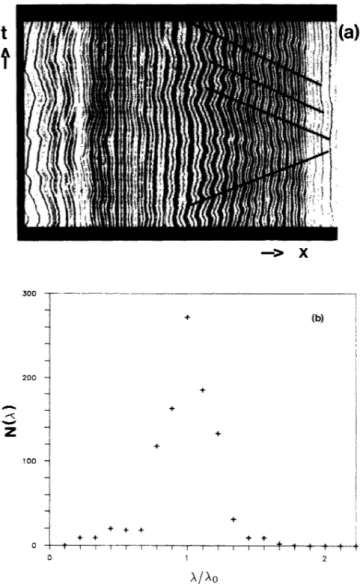
X )I [3 , I I, ,i ) , .) [';ll I'i ~;'I

I-Ii 300 (b) 200 X 100 + + T I I t i & I + + 4 I I t [ I I I I 1 T 1 )/&o

FIG.

5. (a) Same as in Fig. 4but with the annular channel. The total observation time is 1500sec and @=420. Notice at the right and left ofthe frame the crossing ofsolitary waves.

Dark lines indicate the trajectory ofsome solitary waves. (b)

Wavelength distribution at

a=420.

(c)

X

FIG.

4. Space-time evolution ofthe convective pattern ob-tained in the rectangular channel from the shadowgraphic

im-ages. The light intensity is plotted using a gray scale with 256

levels. Spatial digitization is made over 512pixels (horizontal

axis). The total observation time (vertical axis) is 1536 sec.

Vertical dark lines correspond to stationary warm ascending currents. (a)@=350,(b)@=409,(c)@=561.

gate around the container by contamination but they do

not spread. Moreover, they can be separated by very

long periods

of

complete ordered regimes (up to several

hours near

e').

When eis increased, the spatial and

tem-poral extension

of

these domains increases while the

periods

of

ordered regimes become more and more

sel-dom. Around @

=500,

a Auctuating regime made

of LD's

and

TD's

is always present in all the container and is

characteristic

of

sustained intermittency. The

propaga-tion

of

the

TD's

through the pattern

of LD's

has a

tree-like structure (Fig.6) asisobserved in the spatiotemporal

diagrams

of

directed percolation (see

Sec.

V).

Rectangular channel. The transition in the

rectangu-lar cell from the organized "laminar" state tothe

STI

can

be observed in

Fig. 4.

The behavior looks qualitatively

the same as in the annular cell, at least near the

thresh-old, with the coexistence

of

laminar and turbulent

domains, however with a stronger spatial confinement

of

the turbulent regions. As can be seen in

Fig.

4(b),

tur-bulent patches are sandwiched between laminar domains

and hardly propagate throughout the cell.

The simultaneous coexistence

of

two kinds

of

qualita-tively different domains implies the search for acriterion

which distinguishes their different spatial and temporal

42

X

AK48KKR!fall95MIKIIIL4tcktsHF~~ ~ wBlsP.I~' II1'yl)

'%81~85

m491IIIt~~ ' — ~IF4h'I'%II

,~PSSl~

~+~58It'P~' '''apmgag~e,~&0Ic@I ))'s'Mr MlI~~"%El~&

) s- .'ta.~Igloo&~_{~hrcmme ~}

tI ~~Ig(5IIIL'ILiI

mmmm mmmaau s~im a aIIa™.

IRRRSEIElEra\I&A

0.8

0.6

0.4

FIG.

6. Same as in Fig. 4 but with the annular convective pattern at

a=520.

The total observation time is 1000sec (along

the horizontal axis, time is going from left to right) and the spa-tial digitization is made over 250 pixels. Notice the contamina-tion process ofthe turbulent domains throughout the laminar ones. 340 i 380 I 420 I 460 I 500 I 540 I I 580 (b)

periodicity

of

the roll structure is preserved, see Fig. 4(b).

Furthermore, in

LD's

the time evolution

of

the

shadow-graphic intensity

I(x,

t) at a fixed given point is either

stationary or oscillating in time leading to a local

mono-periodic or quasiperiodic regime with a small noise level.

We recall that the oscillations correspond to the

vacilla-tions in the annulus and to ascending plumes in the

rec-tangular cell. On the contrary,

TD's

are regions without

spatial coherence (see Sec. IV B)and their time evolution

ischaotic. This difference between

LD's

and

TD's

iswell

evidenced in Fig. 4(c).

The choice

of

a spatial criterion based on the local

wavelength is therefore justified to discriminate

LD's

from

TD's

without ambiguity. A reduction

of

the signal

can thus be performed, first by finding the extrema

of

the

intensity

I(x,

t) (a maximum corresponding to a cold

stream and a minimum to a hot one). A region in the

convective pattern between two consecutive extrema

x;

and x,

+, of

I

isthen called laminar

if

A,o(—,'

—

b,)&

x;+,

—

_x; &A,_o(—,'

+

6

),

6

being a tolerance factor and A,_o the mean wavelength,

otherwise it is called turbulent. We have checked that

the result does not depend on

6

provided —,'

~

6

~

—,

'.

Such

a choice is suggested by the peaked distribution

of

the

wavelengths as shown in

Fig.

5(b). The signal can then be

reduced to a binary representation

of

I

(laminar or

tur-bulent) which allows us to perform statistics on

LD's

and

TD's.

%'ehave also used a temporal criterion tovalidate

the previous data reductions. Intensity differences

be-tween successive acquisitions were computed and

com-pared toacutoff value

6.

A pixel iiscalled laminar

if

I(i,

t

+1)

I(i,

t)

«5,

—

otherwise it is called turbulent. The results are similar,

but with a larger dispersion, to those obtained with the

spatial criterion. In the following, we present results

0.8

0.6

0.2

I I I l ( l I I I I I I I I I I l

430 470 510 550 590

FIG.

7. Mean turbulent fraction F, as a function of e. (a)

Rectangular channel, (b) annular cell. See text for the full

curves.

which have been computed using the spatial criterion.

In order to characterize the global degree

of

chaos, we

have computed the mean turbulent fraction

_F,

:

F,

refers

to the averaged total length occupied by the turbulent

cells divided by the total length

of

the container.

F,

is

plotted as a function

of

e for the rectangular

[Fig.

7(a)]

and the annular

[Fig.

7(b)]geometry. The difference

be-tween the two geometries is striking even

if

they both

show a continuous increase

of

F,

with

e.

In the

rectangu-lar case, the transition looks like a quasiperfect phase

transition and a fit

of

the experimental data gives the

re-lation

F,

-(e

—

eF

)~,

with eF

=

360 and

P"

=0.

3+0.

05.

In the annular

Notice that in both geometries, no hysteretic

phenomenon has been observed when increasing or

de-creasing the Rayleigh number.

In order to get more information on the nature

of

the

transition and to understand the difference observed in

the two geometries, a detailed statistical analysis has been

made. We present the results separately for each case in

the following.

A. STIinannular geometry

The distributions

of

spatial lengths

of LD's

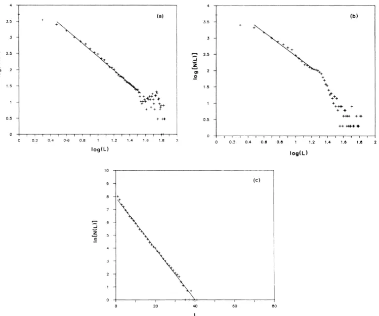
have been

computed. Figure 8 shows the histograms

of

the number

N(L) of

LD's

with length

L

for different values

of

e. One

must notice that the length

L

is computed in term

of

lam-inar cells, so

L

can take values between 1 and 80 in the

annular geometry. When eis varied, two kinds

of

distri-butions are evidenced. In the range

460&

e&500, the

histogram shows a power-law decay, in a domain

of

lengths

L

which is e dependent.

The power-law decay which can be estimated on the

largest available range

of

scales at

e=e,'=480+5

has a

characteristic exponent

p'

=

l.

7+0.

l

[Fig.

8(a)]. Accord-ing to a theoretical definition, ' this value

_e,

'

could be

defined as the threshold

of

STI.

If

we plot the relation

Ft (E E )~ with

P=P"=0.

3 as computed in the

rec-tangular channel, we can fit the experimental points only

at the large values

of e.

The discrepancy observed at the

low values

of

e could be related toanimperfect nature

of

the transition aswill bediscussed in

Sec.

V.

For

e&

_e,

'

the histogram can be divided into two parts:

a first part in the range

of

the small scales shows an

alge-braic decay with the same exponent

_p,

'

while at large

scales an exponential decay isevidenced

[Fig.

8(b)]. The

histograms exhibit this crossover phenomenon until

a=

500,from where they are best fitted by an exponential

3.5 (a) (b) 2.5 X Q) 2 0 1.5 0.5 2.5 Z 4) 2 0 1.5 + + +++ +++ + +tkt +tt ++"~ + I I I'' I 0 0.2 0.4 0 6 0.8 1 1.2 1.4 16 1.8 iog(L) 0.2 0.4 0.S 0.8 1 1.2 1.4 1.S 1.6 log(L) (c) I 20 40 l 60 80

FIG.

8. Histograms

X(L)

oflaminar domains oflength

L.

(a)Power-law distribution at

e=e,'=480,

{b)@=500,(c) exponential distribution at

e=

530.

over the whole range

of

lengths. Figure 8(c}shows this

exponential decay for

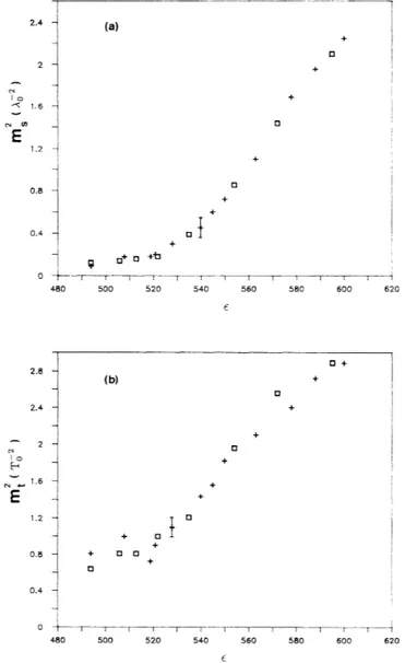
a=530. If

m, is the slope

of

the

curve ln[N

(L

)] versus

L,

the characteristic length

1,

=1/m,

is observed to decrease when e increases. A

plot

of

m, as a function

of

e

[Fig.

9(a)]reveals two kinds

of

behavior: at the lowest values

of

e forwhich m, can be

computed, m, has anearly constant value, while at larger

values

of

e, m, increases almost linearly as a function

of

e.

This linear behavior is similar to the one observed in

the rectangular channel and in the experiment

of

Ciliber-to and Bigazzi. However, the global behavior remains

complex and

if

there exists a transition

—

in the sense

of

phase transition

—

these experimental results evidence its

imperfect nature.

The distributions

of

the lifetime

of LD's

have also been

studied. By analyzing our space-time series with the

same spatial criterion to discriminate laminar from

tur-bulent cells, we have performed histograms giving the

number

N(r)

of

laminar periods lasting

r.

This temporal

approach displays features similar to those obtained in

the spatial distributions. The histogram shows an

alge-braic decay for e',

=490+10

with a characteristic

ex-ponent p',

=2+0.

1, and an exponential decay for e& 500.

The threshold

of STI

is indeed the same (E,

'=e',

) as for

the spatial statistics even

if

the exponents are slightly

different. In the case

of

an exponential decay, a

charac-teristic time l,

=1/m,

is defined and m, varies also

linearly with e

[Fig.

9(b)]

if

we skip the low values

of

6.

B.

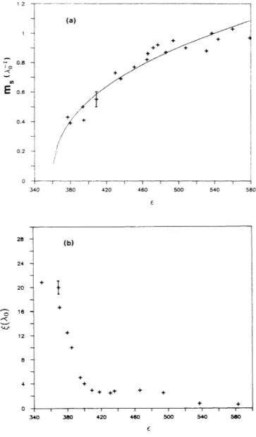
STIinrectangular geometry

2.4 16 1.2 0.4 2.8 2.4 2 Ic) CV 1.2 480 (b) + 0 0 p + + p +b I I t I t I 500 520 540 I I 560 I 1 I 1 580 600 620

We have performed the same spatiotemporal statistical

analysis for the rectangular geometry. The results

hap-pen to be similar to those

of

the annular geometry, except

for the fact that the transition

—

via

STI

—

in this linear

array

of

convective rolls is quasiperfect.

The evolution towards sustained

STI

has been first

quantified via frequency —wave-number power spectra

computed from the temporal evolution

of

the rolls

of Fig.

4.

Near the threshold

of STI

and for increasing

%,

a

large broadening, in wave number, around the mean

wave number is noticed as shown in

Fig.

10(a). At larger

%,

a broadening

of

the peaks takes place in the frequency

domain. We conjecture that this is mainly due to an

un-correlated dynamics

of

the rolls and differs strongly from

the time fluctuations

of

the oscillators. From these 2D

Fourier transforms, no propagation

of

defects, such as

the solitary waves observed near the threshold

of STI,

can be revealed. Such frequency —wave-number spectra

also show that the transition toward sustained

STI

is at

first initiated by a spatial destabilization

of

the uniform

convective pattern giving a wavelength dispersion,

fol-lowed, at higher

A,

by time fiuctuations

of

the new

spa-tial pattern.

The distributions

of

spatial and temporal lengths

of

LD's

exhibit qualitatively the same kind

of

behavior as in

the annular cell. The histograms show a power-law

de-cay near

e=e,

"=360+10,

while they reveal an

exponen-tial decay for

e)

380

[Fig. 11(a)].

The characteristic

length 1,

=1/m,

and time 1,

=

1/m, have a well-defined

dependence on e,as r m,

-(e

—

e,

")

',

a,

"=0.

5+0.

05,

0.4 i

~

i T T I I T I I i I T 480 500 520 540 560 580 600 620

FIG.

9. Annular cell. (a) Square ofthe slope m, computed from the exponential decay of the histograms of the laminar domains, as a function of e. Crosses and rectangles correspond

to increasing and decreasing e, respectively. (b) Square ofthe slope m, computed from the exponential decay of the histo-grams ofthe laminar domains with lifetime ~asa function of e.

m,

—

(E

e,

"}

',

a,

"=0.

5+0.

05 .

—

Probably due to finite-size effects (the container

con-tains only 60 rolls), the power-law distributions are only

defined on a small range

of

scales and therefore it is

diffiicult tofind a precise value

of

_p,

"or

_p,

".

An estimation

gives

_p,

"=1.

6+0.

2and

_p,

"=2.

0+0.

2.

On the other hand, and contrary to the annular case, a unique threshold for

STI

is defined. In fact, the value

of

the threshold

_e,

"

ob-tained from the distribution displaying a power law and

12 0 8 0.6

0

0.2 r-I 340 l 380 I 420 I 460 I 500 I 540 i 580

0

28 (b) 24 20 + p ~ 12

0

+y ++ 420 I I 460 500 + I t I 540 + I SSO

0

FIG.

11. Rectangular cell. (a) Slope m, computed from the exponential decay ofthe histograms ofthe laminar domains, as a function of e. (b)Spatial correlation length g as a function of

e. Notice the strong decrease ofgwhen the convective pattern enters into the spatiotemporal regime at

a=

370.

FIG.

10. 2Dcentered power spectra. Horizontal and vertical

axis are wave-number and frequency axis, respectively. The

maximum wave number and frequency are 1/8 cm ' and 1/6

Hz. The logarithmic power spectra are plotted above a given

threshold. {a)@=380,(b)

a=409.

are the same,

e,

'=eF-

—

360.

This value also corresponds

to

the first events

of

turbulence which can be observed in

the experiment

(e"=350).

Accordingly, the transition via

STI

appears to be almost perfect in the rectangular

con-tainer, but with exponents which do not differ within the

error bars from these

of

the annular geometry.

To

get more information on the transition process, we

have also computed the correlation length _g

of

our

sys-tern. gis defined through the spatial correlation function:

C(r)

=([r(r,

t)

—

(r

&][r(O, t)

—(r

&]

&/(r'),

where

I(r,

t) and

I(o,

t) are the light intensity at two

points separated by a distance rand

( )

denotes the

en-semble average. The envelope

of

the correlation function

C(r)

is expected to decay as

C(r)

—

exp( r_lg

),

—

where g is the correlation length to be compared to the

length

L,

of

the system. As stressed by Hohenberg and

Shraiman,

"

when g&

L,

which is the case for all small

systems, the fluctuations may be regular or chaotic in

for

(

&L„

the dynamical behavior is incoherent in space

and at moderate Rayleigh number is typical

of

a regime

of

weak turbulence without any energy cascade. This is

the case for the convective regime studied in the two geometries.

Correlation functions

of

the intensity were computed

tomeasure the correlation _{length g}for different values

of

e.

The envelopes

of

these functions have an exponential

decay with the distance _{r, from which g can be} extracted.

Fig.

11(b) shows the dependence

of

_{g on} e and reveals a

change

of

behavior near

a=

370,where asudden decrease

of

the correlation length is observed. Below the thresh-old

of STI,

the correlation length is

of

the order

of

the

length

of

the system:

/=20k,

-L„while

far beyond e,

",

(=A, &L,

which corresponds to the observed regime

of

spatiotemporal chaos.

Acharacteristic frequency was also computed from the

first moment

of

the averaged frequency power spectra. '

A monotonic increase

of

the frequency is observed as a

function

of

e; however, no saturation

of

the frequency

value can be seen beyond the sustained

STI

regime.

V. COMPARISON OF EXPERIMENTS

WITH DIRECTED PERCOLATION SIMULATIONS

The results

of

spatiotemporal analysis performed in the

rectangular geometry are typical

of

a second-order phase

transition, but the transition turns out to be imperfect in

the case

of

the annular geometry. The nature and the

characteristics

of

the transition will be discussed in

Sec.

VI.

In this section we compare first the experimental

measurements with available numerical results. Some

statistical properties obtained with a very simple model

constructed from direct percolation are then given.

First

of

all, the experiments reveal the same qualitative

route to turbulence via

STI

as in the numerical

simula-tions

of

some partial differential equations

(PDE

s),

cou-pled map lattices, and directed percolation (DP)and most

of

the characteristic properties observed in the critical

re-gion around the threshold

of STI

are similar to those

ob-tained numerically. The Kuramoto-Sivashinsky equation

with an additional damping term reveals a second-order

transition, with an algebraic decay close tothe threshold,

in the histograms giving the distribution

of

lengths

of

LD's,

' although the critical exponents are different from

the experimental ones. A one-dimensional array

of

maps

coupled by diffusion exhibits also the same behavior. In

this last case, Chate and Manneville have shown that

coupled map lattices display critical properties analogous

to

DP,

but that they do not belong to the same

universali-ty class. The relationship between

DP

and the

transi-tion to turbulence via

STI

had been pointed out by

Pomeau, who has placed the transition toturbulence for

weakly confined systems in the field

of

critical

phenome-na.

To

go further in this comparison between

DP

and

ex-periments, we have performed calculations with a simple

model

of

cellular automaton. In our problem, the

au-tomaton is defined on a 2D lattice: one space dimension

made

of

Nsites (standing for the 1Dgeometry

of

our

ex-periments) plus time. Each site has two possible states: a

laminar state (L) and a turbulent state (T) by

identification, respectively, with a laminar and a

tur-bulent cell in the experiments. The probabilistic rules are

defined on a three-site neighborhood, because the

experi-ments suggest the inAuence

of

the two nearest convective

rolls on the dynamical regime

of

the roll they surround.

The state

of

a celli at time t

+1

thus depends on its state

and on the states

of

its neighbors i

—

1and i

+

1at time t.

In

DP,

the laminar state isabsorbing,

i.e.

,itcannot

be-come turbulent

if

its parents are laminar: _p

(LLL

~T)=0.

However, since the experimental data show

that a turbulent region may originate from a laminar one

around the threshold

of

STI,

a small probability

_p

is

in-troduced so that

p(LLL~T)=p

.

This probability stands for the spontaneous apparition

of

turbulent spots in

LD's.

The automaton is defined by a set

of

eight elementary

probabilities

_Ip„~k

=0,

7I:

p0=p(LLL~T),

p,

=p(LLT~T),

p2

=p

(LTL

~

T), p3

=p

(LTT~T),

p4=p(TLL

~T),

p~

=p(TLT~T),

p6 =p (TTL

~T),

_p7

=p

(TTT~

T)

.

The complementary probabilities are given by the

rela-tion

p(XYZ~L)=1

—

p(XYZ~T)

and because

of

left-right symmetries, we have

_p,

=p4

and p3

=p6. %e

have

chosen the case

of

directed bond percolation, which

seems to be more representative

of

our experiments than

site percolation, because

of

the diffusion process.

More-over, in order to make the calculations easier, we have

taken totalistic rules, ' so that the following relations are

satisfied:

5'I P2 P4

We are thus dealing with only one control parameter

_p

plus the probability

p0=p.

For

the numerical

simula-tions, the number

of

sites N was 10 and the duration

of

the run was several 10

.

The statistical analyses were

per-formed only after some 10 iterations toskip the transient

regimes, especially near threshold. These values are not

large enough to ensure accurate results

of

the exponents,

which also depend on the size

of

the lattice. However,

they allow a description

of

the main characteristics

of

the

studied behaviors.

First

of

all, when

@=0,

the results show a transition

for

_p

=p,

=0.

44. The fraction

of

turbulent sites (the time

average

of

the fraction

of

the system occupied by TD's)

varies as

F,

-(p

—

p,

)'

with

@=0.

28 and, for p

=p„

the histograms giving the

with a characteristic exponent

_p,

(p=0)=1.

5.

More-over, _{for p}

)

p„

the histograms exhibit an exponential

de-cay with a characteristic length l,

=1/m,

which depends

on

p.

The evolution

of

I,

can be fitted by

Q

m,

-(p —

p,

)

', a,

=l

.

The distributions

of

the lifetime

of LD's

evidence the

same transition at _p

=p,

and give an exponent

p,

(p

=

0)

=

1.

6 and a characteristic time l,

=

1/m, for

p

)p,

.

m,

dependsonpas

0.8

0.8

0.4

m,

—

(p

—

p,

)

',

a,

=l

.

A correlation length _g can also be defined from the spa-tial correlation function which decays as

C(r)

-exp(

—

r/g).

The variation

of

_{g reveals} a transition

near

_p

=p,

which varies as

0.2

0 I I t i i t I I I I I I I t I t I

0.38 0.4 0.42 0.44 0.46 0.48 0.5 0.52 0.54

with v,

=0.

5. A second-order phase transition is

there-fore observed when

_p

=0,

with well-defined threshold and

characteristic exponents.

The results obtained when pWO display several

impor-tant differences from the _{case p}

=0.

First

of

all, the

spa-tiotemporal representations

of

the automaton exhibit

features very similar to the experimental results.

It

shows the importance

of

the spontaneous appearance

of

turbulent sites for the generation

of

localized

TD's

near

the threshold

p„while

for p

&&p„

the role

of

_p is totally

hidden by the process

of

contamination

of LD's

by

TD's.

The statistical properties are also changed by the pres-ence

_{of p.}

If

it is small enough (p

(10

), an algebraic

decay is still observed in the histograms giving the

distri-bution

of LD's,

but in a range

of

length scales which

shortens when _{p increases.} The characteristic exponent

also depends on

p.

With

p=5X10,

the histograms

show an algebraic decay around _p

=0.

44 on 100 sites

with acharacteristic exponent

_p,

(p

=5X10

)

=1.

4.

On

the other hand, no noticeable change is observed in the

distributions

of

lifetime

of LD's,

provided _p is small

enough:

_p,

(p=

0)=p,,

(P=

5X1

0

). When _p is

in-creased further, no transition in the functional form

of

the distributions

of

LD's

is observed: all the histograms

show an exponential decay. This last result is similar to

the conclusions

of

Bagnoli et

al.

,' who have also

com-pared the behavior

of

the experimental data

of

Ciliberto

and Bigazzi with that

of

suitable chosen automaton

rules.

When

p&0,

achange

of

behavior

of

the turbulent

frac-tion is still observable (Fig. 12). The value

of

I',

_{for p}

=p,

is different from zero and increases with

p.

In fact,

if

p &

10,

F,

evolves slowly with p and reveals no

transi-tion. The evolution

of

m, (or m,) with _p is also affected

by an increase

of

p, as the evolution

_{of F,}

.

In conclusion, these numerical results show the

ex-istence

of

a well-defined transition in the case

of

directed

percolation,

i.e.

, when the laminar state is absorbing

(p

=0).

When the laminar state is quasiabsorbing

(P&0),

the transition disappears in a strict sense or becomes

im-perfect. The evolution

of

the turbulent fraction becomes

FIG.

12. Mean turbulent fraction F, as a function of the probability _p for different _p (see text). Squares, P'=0; crosses,

p

=

5X

10;

diamonds, p

=

10

',

triangles, _p

=2

X 10

smooth; meanwhile, the algebraic decay, which is

charac-teristic

of

the critical transition, disappears when _p

in-creases.

Finally, these numerical results performed on a very

simple model

of DP

give an interesting insight on the

ex-perimental data. The rectangular geometry is well

represented bypure

DP;

meanwhile, the annular case can

be compared to

DP

with pAO. Though the physical

na-ture

of

_p is not explained, it gives a good representation

of

the spontaneous apparition

of

turbulent cells. As a

power-law decay is present in the experimental

distribu-tions, it turns out that the probability p issmall in the

ex-periments, as shown by the numerical results. The

lami-nar state

of

the convective rolls isthus quasiabsorbing.

VI. DISCUSSION

The experimental results discussed in this paper have

shown that in quasi-1D Rayleigh-Benard convection, the

evolution

of

the convective state to sustained spatial

tur-bulence is achieved through the development

of

spa-tiotemporal intermittency, as expected from theoretical

and numerical studies. The observation and quantitative

analysis

of STI

regimes have been previously performed

in convection experiments, but in that case, the 1D

character was not well fulfilled, and the criterion to

separate

LD's

from

TD's

was different from that used in

the present study. Nevertheless, many properties remain

similar in the two cases, showing the robustness

of

the

STI

regimes.

In the present study, two different geometries were

used. Periodic boundary conditions were obtained using

an annular cell, while fixed boundary conditions prevailed

in the rectangular channel. The transverse aspect ratio

was slightly different for the two cases, but this difference

preced-ing

STI.

As a matter

of

fact, the first time-dependent

convective behavior was given by the appearance

of

oscil-lators in the convective pattern

—

plumes in the

rectangu-lar channel, vacillations in the annulus

—

in agreement

with the general observation that vacillations donot exist

when I"

)

0.

4.

Nevertheless, the qualitative behavior

of

the sustained

STI

regime was exactly the same in both

geometries, therefore it is independent

of

the nature

of

the oscillators in the convective pattern. Their infiuence

on the

STI

threshold through eventual specific

mecha-nisms

of

spatial destabilization is unknown, but it is likely

that the observed difference

(e"=360, e'=480)

is related

only to the value

of I'

itself (in the experiment reported

in

Ref.

7,the threshold value

e'=200

with

I

=

1).

In the two geometries, the spatiotemporal intermittent

regime corresponds

to

a loss

of

spatial coherence and

ap-pears as an interspersing

of

turbulent patches within

lam-inar domains. Very close

to

the

STI

threshold, turbulent

patches spontaneously appear from time to time and,

after a while, relax and disappear. The intermittent

be-havior

of

a complete ordered pattern with a locally

tur-bulent one is observed within a very narrow einterval in

the rectangular channel, and within a larger

e

domain in

the annulus, as isclearly evidenced by the variation

of

the

turbulent fraction as afunction

of e.

Moreover, this

vari-ation shows that in the former case, we have a

quasiper-fect second-order phase transition. In the case

of

the

an-nulus, the nature

of

the transition from laminar state to

STI

is more complex and looks imperfect, though the

statistics concerning the length

of

the laminar domains

(power law at the "effective" threshold, scaling law for

the characteristic length) are similar to the statistics

ex-pected for awell-defined transition. A somewhat similar

behavior has been reported in

Ref.

7, where the

convec-tion isalso built up in an annular container (with

I

=1).

The striking difference between the behaviors in the

an-nular and rectangular geometries is probably due to the

influence

of

the boundaries which stabilizes the phase

of

the rolls in the rectangular channel. On the contrary, in

the annular geometry, an intrinsic phase roll instability

together with a possible large scale flow could induce the

observed imperfect transition. In fact, it is only in this

geometry that turbulent patches propagate near the

threshold.

The experimental results agree globally with those

ob-tained by numerical simulation

of

PDE

or coupled maps

and also with directed percolation. The quantitative

comparison between the values

of

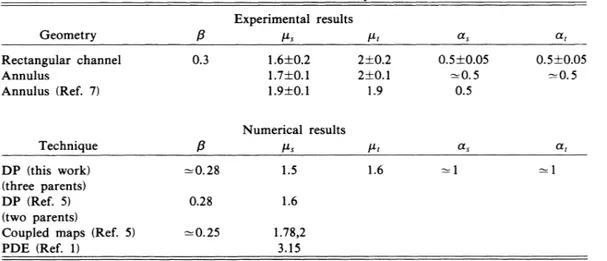
the exponents

numeri-cally and experimentally measured (see Table I) is not

straightforward, for recent

studies"

show that the

ex-ponents are not universal. They depend, in particular, on

the size

of

the system, but also on the underlying

mecha-nisms which govern the transition. Nevertheless, the

ex-ponents

P'

—

for the evolution

of

the turbulent fraction in

the rectangular geometry

—

and

_p,

—

of

the algebraic

decay

—

deduced from the experimental observations,

may agree with those

of DP

and coupled maps.

To

our

knowledge, the prediction concerning the u exponent

describing the evolution

of

the inverse

of

the

characteris-tic length as a function

of

e, has not yet been done. The

exponent obtained through our numerical simulation

of

directed percolation is not the same as from the

experi-mental data. Furthermore, no clear correspondence

be-tween the two control parameters _p and

e

can be

estab-lished. A recent phenomenologica1 study

of

a 1D chain

of

rolls, performed in the frame

of

the

Landau-Ginsburg equation, ' could give a transition similar to

our experimental observations.

The recent studies

of

1D periodic systems have

re-vealed the richness

of

their spatial and dynamical

proper-ties. In a certain range

of

the control parameter, they

present an analogy with a chain

of

coupled oscillators,

and so, are linked to dynamical systems. Then, the first

symmetry breaking

of

the space translation takes place

by the appearance

of

propagative solitary waves. These

waves, observed in the convective narrow channels, have

been also evidenced in directional solidification ' _{and in}

the periodic front

of

the meniscus

of

afiuid between two

rotating cylinders. In this last experiment,

spatiotem-poral intermittency is also currently under investigation.

Therefore it seems that a large amount

of

the properties

we have found is generic to 1Dsystems.

Geometry

TABLE

I.

Values ofdifferent exponents Experimental results Ps Rectangular channel Annulus Annulus (Ref. 7) 0.3 1.

6+0.

2 1.

7+0.

1 1.

9+0.

1

2+0.

2

2+0.

1 1.9 0.

5+0.

05

=0.

5 0.5 0.

5+0.

05

=0.

5 Technique DP (this work) (three parents) DP (Ref. 5) (two parents)

Coupled maps (Ref. 5)

PDE (Ref. 1)

=0.

28 0.28

=0.

25 Numerical results 1.5 1.6 1.78,2 3.15 1.6

a,

ACKNOWLEDGMENTS

We wish to acknowledge

G.

Balzer,

P.

Berge,

R.

Bi-daux,

Y.

Pomeau, and

P.

Manneville for fruitful and

stimulating discussions. We would like to thank also

P.

Hede for the development

of

the image processing and

B.

Ozenda forhis technical assistance.

H. Chate and P.Manneville, Phys. Rev. Lett. 58, 112 (1987).

According to a private communication with one ofthese au-thors, P.Manneville, the knowledge ofthe exact nature ofthe transition, studied inthis paper, requires more studies.

U. Frisch, Z. S.She, and O. Thual,

J.

Fluid Mech. j.68, 221

(1986).

B.

Nicolaenko, Nucl. Phys. B(Proc. Suppl.)2, 453 (1987); H.

Chate and

B.

Nicolaenko, in New Trends in Non-Linear

Dy-namics and Pattern Forming Phenomena: the Geometry of

Nonequilibrium, edited by P.Huerre and P.Coullet (Plenum,

New York, 1990).

4K.Kaneko, Prog. Theor. Phys. 74, 1033(1985).

5H. Chate and P.Manneville, Physica D 32, 409 (1988);

J.

Stat.

Phys. 56,357(1987).

P.Berge, Nucl. Phys. B2, 247(1987).

7S. Ciliberto and P.Bigazzi, Phys. Rev. Lett. 60,286(1988).

F.

Daviaud, M. Dubois, and P.Berge, Europhys. Lett. 9,441

(1989).

Y.Pomeau, Physica D23,3(1986).

' _{M. Dubois, P.Berge, and A. Petrov, in New Trades in} Non-Linear Dynamics and Pattern Forming Phenomena: the

Geometry

of

Nonequilibrium, edited by P. Huerre and P.

Coullet (Plenum, New York, 1990).

'

_J.

_E.

_{Wesfreid and V. Croquette, Phys. Rev. Lett. 45, 634}

(1980); V. Croquette and

F.

Schosseler,

J.

Phys. 43, 1183

(1982).

' _M.Dubois,

_R.

_{Da Silva,}

_F.

_{Daviaud, P.Berge,and A.Petrov,}

Europhys. Lett. 8, 135(1989).

' _M.Dubois,

_F.

_{Daviaud, and M. Bonetti, in Non-LI'near}

Evolu-tion ofSpatio Temp-oral Structures in Dissipative Continuous

Systems, edited by

F.

H.Busse and

K.

Kramer (Plenum, New

York, 1989).

' _{H.Chate, Ph.D.thesis, University ofParis, 1989.}

' _{P. C. Hohenberg and}

_B.

_I.

_{Shraiman, Physica D 37, 109}

(1989).

J.

P. Gollub and

R.

Ramshankar, Ne~ Perspectives in

Tur-bulence, edited by S.Orszag and L.Sirovich (Springer-Verlag,

Berlin, in press).

W.Kinzel, Ann. Israel Phys. Soc. 5,425(1983)~

'

_F.

_{Bagnoli, S.Ciliberto, A. Francescato,}

_R.

_{Livi, and S.Ruffo,}

in Chaos and Complexity, edited by

R.

Livi, S.Ruffo, S.

Cili-berto, and M.Buiatti (World Scientific, Singapore, 1988). 9R.Bidaux, N. Boccara, and H. Chate, Phys. Rev. A 39, 394

(1989).

P.Coullet and G.Iooss, Phys. Rev.Lett.64, 866(1990).

J.

Lega and P.Coullet (private communication).

A.

J.

Simon,

J.

Bechhoefer, and A. Libchaber, Phys. Rev.

Lett. 61,2574(1988);P.Coullet,

R. E.

Goldstein, and G.H.

Gunaratne, ibid. 63, 1954 (1989).

G.Faivre, S.de Cheveigne, C.Guthmann, and P.Kurowski, Europhys. Lett. 9, 779 (1989).

M. Rabaud, S.Michalland, and

Y.

Couder, Phys. Rev. Lett.