Concept development for lightweight binary-actuated robotic devices, with application to space systems

(1)

Concept Development for Lightweight Binary-Actuated Robotic Devices, with Application to Space Systems

by

Matthew D. Lichter

B.S. with Honors, Mechanical Engineering The Pennsylvania State University, 1999

Submitted to the Department of Mechanical Engineering in Partial Fulfillment of the Requirements for the Degree of

Master of Science in Mechanical Engineering at the

Massachusetts Institute of Technology June 2001

BARKER D Massachusetts Institute of Technology

/7

MASSACHUSETTS INSTITUTE_{MASSACHUSETTS}_INSTITUTE OF TECHNOLOGY

JUL 16 2001

LIBRARIES Signature of Author ... . ...

Department of Mechanical Engineering May 11, 2001

Certified by ...

Accepted by ...

Chai

Skeven Dubowsky Professor of Mechanical Engineering Thesis Supervisor

Ain A. Sonin rman, Department Committee on Graduate Students

(2)

Concept Development for Lightweight Binary-Actuated Robotic Devices, with Application to Space Systems

by

Matthew D. Lichter

Submitted to the Department of Mechanical Engineering on May 11, 2001 in Partial Fulfillment of the

Requirements for the Degree of Master of Science in Mechanical Engineering

ABSTRACT

Exploratory space missions of the future will require robotic systems to lead the way by negotiating and mapping very rough terrain, collecting samples, performing science tasks, and constructing facilities. These robots will need to be adaptable and reconfigurable in order to achieve a wide variety of objectives. Conventional designs using gears, motors, bearings, encoders, and many discrete components will be too complex, heavy, and failure-prone to allow highly-reconfigurable systems to be feasible.

This thesis develops new concepts that may potentially enable the design of self-transforming space explorers. The vision of this research is to integrate compliant bistable mechanisms with large numbers of binary-actuated embedded smart materials. Compliant mechanisms are lightweight and robust. Binary actuation is the idea of using an actuator in a discrete on/off manner rather than in a continuous manner. A binary actuator is easy to control and robust, and by using tens or hundreds of binary actuators, one can approximate a continuous system, much like a digital computer can approximate an analog system.

The first part of this thesis examines the fundamental planning issues involved with systems having large numbers of binary actuators. The notion of a workspace is described and applied to the optimization of a manipulator design. Methods for solving the forward and inverse kinematics are discussed in the context of this application. These methods are extended to the trajectory and locomotion planning problems. Methods for planning systems of substantial complexity are developed in the context of exploratory space robotics.

The second part of this thesis presents experimental demonstrations that examine elements of the concept. The results of several design prototypes are discussed.

Thesis Supervisor: Steven Dubowsky Title: Professor of Mechanical Engineering

(3)

ACKNOWLEDGEMENTS

I would like to thank the MIT Rosenblith Fellowship, the Department of Defense, the NASA Institute for Advanced Concepts, and the NASA Jet Propulsion Laboratory for their support of this research. I would like to thank collaborators on this research program, including Dr. Gregory Chirikjian, Dr. John Madden, Dr. Ian Hunter, Mr. Roy Kornbluh, and Dr. Paul Schenker. Special thanks go to all the members of the Field and Space Robotics Laboratory, whose help was greatly appreciated at one point or another

-Chris for his programming help, Vivek for his pearls of wisdom, Moustapha for his collaboration, Ebraheem for his machining skills, and all the rest of the members for making the FSRL a stimulating and enjoyable research environment. And of course, thank you Dr. D for the opportunity and the mentorship to work on a great project.

Thanks especially to my family - Mom, Dad, Pete, Sharon, and Jim - whose

support has always made things possible. Thanks to my friends for keeping it real and thanks to Brittany for keeping me (in)sane.

(4)

FIGURES

1.1. Martian terrain as seen from the NASA Pathfinder lander, 1997.

(C ourtesy JPL .)... 11

1.2. (a) Sojourner rover that landed on Mars in 1997; (b) Rocky 7 test bed rover, one of many currently used to test technologies and concepts on E arth. (C ourtesy JPL .)... 12

1.3. Simulation of Sojourner, showing the difficulty in surmounting obstacles with conventional technologies. (Courtesy JPL.)...12

1.4. The benefits of self-transformation. [Andrews, 2000]...13

1.5. Vision of a self-transforming explorer (STX) composed of modules and articulated elements. [Andrews, 2000] ... 14

1.6. Flexure-based elastic hinges: (a) notch flexure; (b) beam flexure. ... 15

1.7. Compliant pincer mechanisms. [Ananthasuresh] ... 18

2.1. (a) Continuous robot and workspace; (b) binary-actuated robot and discrete w orkspace... 22

2.2. Transformation of a discrete point cloud to a continuous density representation using a low-pass (Gaussian) filter...24

2.3. A binary serial manipulator, showing the design variables li, 80j, and pj that can be optimized to provide uniform workspace density...25

2.4. A 6-DOF serial binary manipulator, optimized for uniform workspace density, showing a few binary configurations (top), and its workspace density m ap (bottom ). ... 27

2.5. Coordinate frames of each module within a binary device...28

2.6. BRAID: a serial chain of binary-actuated parallel stages...29

2.7. Potential BRAID applications: (a) mating two rovers; (b) maneuvering an instrum ent... . 30

2.8. Comparisons between basic crossover methods...35

2.9. Stage crossover vs. bit crossover... 36

2.10. Inverse kinematics solution times for various algorithms...38

2.11. Representative workspace of a 30-DOF BRAID. 1000 random target points were chosen from within the working workspace, a sphere whose size is slightly smaller than the actual workspace cloud...39

2.12. Error distributions for a 30-DOF BRAID: displacement error (left); angular error (right). (1000 samples.)...40

(7)

2.13. Median errors vs. number of DOF for different algorithms: displacement

error (left); angular error (right). (1000 samples per DOF.) ... 40

2.14. A smooth trajectory in Cartesian space is not necessarily smooth in configuration space ... 42

2.15. Inverse kinematics solution times as they relate to the trajectory following problem . ... . . 43

2.16. Simulation of a camera maneuvering task using the trajectory-planning algorithm. Desired trajectory: red path; actual trajectory: green path. ... 44

2.17. Simulation of a 6x21-DOF walking robot composed of six BRAIDs for legs, walking in rough terrain... 45

2.18. Kinematic models in simulation: (a) rigid; (b) semi-compliant. ... 46

2.19. Computational process for planning the trajectories for each leg. ... 48

2.20. Equilibrating the rigid robot to the ground in simulation: the potential energy in the springs is minimized. ... 48

3.1. Bistable rotary joint designs: (a) spring-loaded over-throw mechanism; (b) detent-based latching mechanism ... 53

3.2. Bistable joint: a sandwich of bistable members and elastic hinges...54

3.3. B istable joint prototype... 54

3.4. Various amplification mechanisms...56

3.5. Pantograph mechanism schematic...57

3.6. Pantograph mechanism prototype...57

3.7. Single stage of first BRAID prototype. [Sujan, et al, 2001] ... 58

3.8. First generation BRAID prototype. [Oropeza, 1999] ... 59

3.9. Tentative design of a second generation BRAID. (Courtesy M. Hafez.) ... 60

3.10. Test prototype of an unactuated single BRAID stage... 61

C. 1. One stage of the BRAID, showing its eight binary configurations. ... 77

C.2. Coordinate frames for a single stage...78

C.3. (a) Axes of revolution of the five flexural hinges in one link of a stage; (b) hinge angle definitions ... 79

C.4. Geometry of stage in state 000...79

C.5. Geometry of stage in state 111...80

C.6. Geometry of stage in state 100...81

C.7. Geometry of stage in state 010. ... 83

C.8. Geometry of stage in state 001...84 7

(8)

C.9. Geometry of stage in state 011. ... 85

C.10. Geometry of stage in state 101. ... 87 C.11. Geometry of stage in state 110 ... 88

(9)

CHAPTER

1

INTRODUCTION

1.1 Introduction

This thesis presents preliminary concept development for a new lightweight, robust robotic design paradigm, with special emphasis on space applications. The work presented here represents the author's contribution to a collaborative research program being carried out at the MIT Field and Space Robotics Laboratory. This program is funded by the NASA Institute for Advanced Concepts (NIAC), an autonomous agency created to "provide an independent open forum for the external analysis and definition of space and aeronautics advanced concepts [and] complement the advanced concepts activities conducted within the NASA Enterprise" [NASA Institute for Advanced Concepts, 2001]. The NIAC is focused on supporting research that may dramatically impact the aerospace community on the 10 to 40 year time horizon and strongly seeks research programs that show promise for leapfrogging current technology development.

The design paradigm being explored and developed in this laboratory involves using compliant, elastic structures embedded with a large number of simple binary actuators. A binary actuator is one that is capable of robustly maintaining only two discrete states: an on or an off position. This is in contrast to conventional robotic devices, which use continuous actuators such as motors, hydraulics, pneumatics, etc. A binary actuator could be made of a lightweight smart material such as shape memory alloy (SMA), conducting polymer, electrostrictive polymer, piezo polymer, etc.

Chapter 1. Introduction 99

(10)

The use of a large number of binary actuators as opposed to a few continuous ones is analogous to the leap from analog to digital computing. By using tens, hundreds, or thousands of binary actuators, one can approximate a continuous system in dexterity and utility. Incorporating simple compliant mechanisms, rather than complex gear trains, bearings, and lubrication, vastly reduces the number of moving parts and hence increases robustness. Further design additions, such as the use of simple bistable mechanisms to reinforce the actuator commands, provide additional robustness.

While compliant mechanisms and binary actuators are not new concepts, their combination in large numbers to create robotic systems has not been studied. The goal of this study was to examine the fundamental issues and challenges involved with this compliance-based binary robotic paradigm. The research discussed here explores the planning and control issues involved with highly redundant binary systems as well as

some of the preliminary challenges in building such devices.

1.2 Motivation

The exploration and development of the planets and moons in our solar system in the next 10 to 40 years are stated goals of NASA and the international space science community [NASA, 1998]. In order to do this, robotic systems will need to lead the way by scouting, collecting geologic samples, mapping, performing science tasks, and constructing facilities, while working in highly unstructured environments and negotiating very rough terrain [Huntsberger, et al, 2000] (see Figure 1.1).

(11)

Figure 1.1. Martian terrain as seen from the NASA Pathfinder lander, 1997. (Courtesy JPL.)

Current planetary robotic systems do not have the capabilities to perform these missions. They are rovers or landers, built with a fixed configuration, capable of functioning in benign terrain and performing specific surveying and minor sample collection. They are composed of a large number of mechanical and electrical components such as gears, motors, bearings, encoders, and sensors. The latest planetary rover, Sojourner, and those under development are relatively conventional fixed-configuration vehicles carrying a simple mechanical manipulator [Bickler, 1992; Schenker, 1997] (see Figure 1.2). This technology, while well conceived for current and near-term science objectives, will not meet the demands of missions forecast for the new millennium. Even relatively small rocks the size of the rover itself present serious obstacles to current rovers (see Figure 1.3). They will not be able to explore rough terrain, such as cliff sides, deep ravines, and craters, where the most interesting scientific samples and information are probably located. Nor will they be able to perform even the simplest assembly or construction tasks.

(12)

Figure 1.2. (a) Sojourner rover that landed on Mars in 1997; (b) Rocky 7 test bed rover, one of many currently used to test technologies and concepts on Earth. (Courtesy JPL.)

Figure 1.3. Simulation of Sojourner, showing the difficulty in surmounting obstacles with conventional technologies. (Courtesy JPL.)

Rather than implementing exploratory robots in a fixed-configuration manner with highly specified tasks, robots of the future will need to be adaptable, transforming themselves to meet a wide variety of objectives when needed (see Figure 1.4). A robot

(13)

that is optimized for adaptability, rather than a few specific tasks, will be much more valuable and cost-effective for missions of the next 10 to 40 years. Unfortunately, conventional components such as gear trains, motors, bearings, and encoders will render self-transformation unfeasible, due to their complexity, weight, and proneness to failure. New robot technology concepts as well as new paradigms for the design of space robots are required to meet the needs of future planetary exploration and development programs.

Figure 1.4. The benefits of self-transformation. [Andrews, 2000]

1.3 The Self-Transforming Explorer (STX) Concept

The thrust of the project being carried out by the MIT Field and Space Robotics Laboratory is to develop the fundamental planning and component technologies to enable the concept of self-transforming exploratory (STX) robots. Figure 1.5 shows such a robot, as envisioned by this research group, which is composed of modules interconnected by generic articulated elements [Andrews, 2000]. With such a structure, interconnections between different modules could be formed or broken to create a wide

13 Chapter 1. Introduction

(14)

variety of topologies, thus providing a diversity of capabilities. The articulated elements would not be composed of conventional gears and motors, but rather would be made from a compliant structure embedded with smart material actuators. The number of discrete parts would be substantially reduced, thus improving robustness in hostile environments and simplifying overall design and fabrication. Specifically, the vision laid out by this research group consists of four main points: embedded muscle-type actuators; polymer-based compliant mechanisms; binary actuation and control; and bistable joints and structures. These will be discussed in detail in the following subsections.

Figure 1.5. Vision of a self-transforming explorer (STX) composed of modules and articulated elements. [Andrews, 2000]

1.3.1 Embedded Muscle-Type Actuators

The first point of the STX vision is the concept of embedded muscle-type actuators. Researchers are presently developing a wide variety of smart muscle-like actuators, including conducting polymers, dielectric (electrostrictive) polymers, piezo polymers, shape memory alloys, polymer gels, and ferromagnetic polymers [Madden, et al, 2000; Pelrine, et al, 1998, 2000; Waram, 1993; Jolly, et al, 1996]. In the 10 to 40 year timeframe, many materials such as these will be developed into commercial engineering technologies. These technologies have the potential for revolutionizing a variety of mechanical systems, as they are lightweight, compact, and often lead to highly integrated designs due to their fundamental simplicity. In addition, these materials have the

(15)

potential for being very robust, as they typically consist of only a few components. Fewer components generally equates to a lower likelihood of system failure.

1.3.2 Polymer-Based Compliant Mechanisms

The second facet of the STX vision is the concept of replacing conventional bearings and sliding surfaces with flexures and compliant mechanisms (see Figure 1.6). The notion of compliance in mechanisms is not new, and much research has gone into developing methodologies for their design and optimization [Midha, et al, 1992; Ananthasuresh, et al, 1995; Frecker, et al, 1996, 1999]. They have seen limited use in robotic systems, however. While often not as stiff as ball bearings, they have the advantage of simplicity, light weight, low cost, zero friction, and no moving parts. Having a finite range of motion, they match nicely with muscle-type actuators, whose motions are also bounded. One can fabricate a large number of compliant joints into a single piece of material, reducing the assembly requirements for the device as well as the total part count. Methods are also being developed for embedding actuators during the fabrication of compliant mechanisms and structures [Madden, et al, 1995; Cham, et al, 1999]. Again, by their fundamental simplicity, compliant mechanisms can be very reliable, an important trait in the application of exploratory space systems.

Figure 1.6. Flexure-based elastic hinges: (a) notch flexure; (b) beam flexure.

1.3.3 Binary Actuation and Control

The third component of the STX vision is the notion of binary actuation and control. Binary actuation refers to using actuators in a discrete manner, such that each actuator is capable of maintaining only two states - an on or an off position. Actuators can be designed to maintain these states reliably and precisely without the use of

(16)

feedback control. By using a large number of binary actuators, as opposed to a few continuous ones (motors, hydraulics, etc.), one can approximate a conventional system in dexterity and utility. This is analogous to the leap from analog to digital computing. Large networks of binary smart-material actuators could be embedded in compliant structures in a manner similar to the mass production of computer processors and circuit boards. In addition to their potential robustness, binary actuators lend themselves well to digital computation and control. A completely binary system avoids the complexity of analog-to-digital conversion, and control commands to the actuators are a simple 1 or 0. More importantly, control commands are insensitive to noise and precise signal commands are not necessary. That is, a binary system using digital logic will recognize any command signal above a certain threshold as a 1, and anything below as a 0. As long as command signals are kept well above or below thresholds, noise and imprecision in the actual command voltage have no affect on system behavior.

1.3.4 Bistable Joints and Structures

The fourth element of the STX vision is the idea of bistability in the mechanical structure and joints. A bistable mechanism is one that exhibits stability in two of its states, maintaining its configuration in the presence of disturbances [Iqbal, Pellegrino, 2000]. An example of this is a household light switch. In either the on or off position, the switch reliably maintains its mechanical position. An ideal bistable mechanism is unstable between its two stable states. The purpose of bistable mechanisms in binary robotic devices is to reinforce the desired state of the binary actuator and to increase the stiffness of the system when in a fixed configuration. When designed properly, a bistable mechanism in parallel with a binary actuator allows the controller to shut off power to the actuator, relying on the passive bistable mechanism rather than the actuator to reject disturbances. This is important for systems with a large number of actuators, when power is to be conserved.

The synergistic combination of embedded muscle-type actuators, compliant mechanisms, binary actuation and control, and bistable mechanisms provides a framework for a new design paradigm in lightweight robotic devices. This new approach

16 Chapter 1. Introduction

(17)

to space robotics may enable the design of increasingly complex exploratory robots, capable of adapting to a variety of mission requirements.

1.4 Background and Literature Review

Most of the elements of the STX vision are not new ideas and have been researched to varying degrees over the last ten to twenty years. However, to date the synergistic combination of all these elements has not been examined outside of the MIT Field and Space Robotics Laboratory [Oropeza, 1999; Dubowsky, 1999; Andrews, 2000; Lichter, et al, 2000; Sujan, et al, 2001].

The notion of using compliance to replace sliding parts is not at all new (consider a bow and arrow), but extensive research in this area over the last decade has produced very interesting results. The rapid growth of plastics use in this century has brought about a wide variety of implementations, such as tweezers, pincers, and mechanisms with a fixed (and often small) range of motion (see Figure 1.7). More recently, compliant mechanisms have been incorporated into MEMS devices, where alternative methods such as bearings are extremely difficult to build [Jensen, et al, 1997], and in surgical devices, where the simple monolithic nature of the device lends itself well to sterilization [Canfield, et al, 1999; Cappelleri, et al, 1999]. The notion of bistability in compliant and composite structures has also been explored [Jensen, 1998; Opdahl, et al, 1998; Iqbal, Pellegrino, 2000]. In recent years, automated design procedures have been developed to produce and optimize mechanism topologies and geometries based on given functional requirements [Midha, et al, 1992; Howell, et al, 1994; Murphy, et al, 1994; Ananthasuresh, et al, 1995; Frecker, et al, 1996, 1999; Saggere, et al, 1997; Hetrick, et al, 1998]. Design solutions generated by computer optimization have often led to very unusual and clever mechanisms.

(18)

Figure 1.7. Compliant pincer mechanisms. [Ananthasuresh]

A very large area of research in the last ten years has been the area of artificial muscle technology. The preponderance of materials research groups around the world has led to a wide variety of potential actuation technologies. Conducting polymers and gels use the diffusion of ions into their molecular structure to change shape and volume [Madden, et al, 1995, 2000; Baughman, 1996]. Dielectric or electrostrictive polymers change shape under the electrostatic force of charge stored on parallel conductive plates [Kornbluh, et al, 1999; Pelrine, et al, 1998, 2000]. Ferromagnetic polymers change shape through the use of a magnetic field in conjunction with ferrous particles embedded in an elastomer matrix [Jolly, et al, 1996]. Shape memory alloys are metal alloys that change their crystalline structure, and thus their shape, under the application and removal of heat [Waram, 1993; Gilbertson, 1994; Youyi, Tu, 1994]. This is only a small sample of the many different materials that have been explored recently; even more will certainly follow.

The notion of embedded actuation and sensing is a somewhat new idea. Several groups have explored active damping and shape control of composite structures using embedded shape memory alloys [Baz, et al, 1994; Lee, Sun, 1995]. Similar studies have been performed with plastics and piezoelectric materials [Agrawal, et al, 1994]. The embedding of shape memory alloys and conducting polymer actuators for robotic and deployment applications has also been studied [Della Santa, et al, 1996; Wang, Shahinpoor, 1996; Huang, Pellegrino, 1996]. Methods of embedding discrete

Chapter 1. Introduction 18

(19)

components or actuators into plastic structures during manufacture have also been explored in a few places with interesting results [Madden, et al, 1995; Cham, et al, 1999].

Various groups have studied the concepts of modular reconfigurability, robotic cooperation, and autonomous organization in recent years. Extensive simulations and some experimental studies have demonstrated autonomous planning algorithms for general systems composed of tens or hundreds of "molecular" modules [Kawauchi, et al, 1992; Kotay, et al, 1998]. Self-assembly of systems has also been studied [Murata, et al, 1994]. Metrics for planning modular reconfiguration have been developed [Pamecha, et al, 1997]. Several groups have studied modular reconfiguration of manipulators, snake-like robots, and exploratory robots [Yim, 1995; Farritor, et al, 1996, 1997; Kotay, Rus, 1997; Hirose, 2000]. The architectures themselves of such modular systems have been a focus of considerable attention [Tesar, Butler, 1989; Farritor, 1998].

Of the different components of the STX vision, the area of binary robotics has seen the least amount of research. Some preliminary work in discretely actuated robots occurred many years ago [Pieper, 1968; Roth, et al, 1973; Koliskor 1986], but further research faded due to the lack of computation power available at the time. More recently, related research has been done in the areas of sensor-less manipulation and discrete command architectures [Erdmann, Mason, 1988; Goldberg, 1992; Canny, Goldberg, 1993]. The planning, control, and analysis of binary robotic systems has been studied primarily by a small number of research groups [Chirikjian, 1994, 1995, 1997; Ebert-Uphoff, et al, 1996; Lees, Chirikjian, 1996; Chirikjian, et al, 1998; Kyatkin, et al, 1999; Suthakorn, et al, 2000; Lichter, et al, 2000; Sujan, et al, 2001].

What has yet to be studied in great detail is the combination of all of these elements in large numbers to create a robotic device. Compliant mechanisms, embedded actuators, smart materials, bistable mechanisms, hyper-redundant binary robotics, and reconfigurable systems are all fairly well studied but have never been completely integrated by any one project. It is therefore the aim of this research program to examine systems combining all these elements.

(20)

1.5 Research Overview

Because the STX concept is intended for implementation in the 10 to 40 year time horizon (in accordance with the NIAC objective), it is impossible to create a complete example of the STX vision through the course of this research. However, one can demonstrate fundamental aspects of the planning, control, design, and fabrication of representative robotic subsystems. The goal of this research, then, is to use simulation studies to demonstrate feasibility for the planning and control of binary robotic systems, and to use preliminary laboratory experiments to examine issues involved in their design and fabrication. This work seeks to identify aspects of the vision that are achievable today, those that show promise in the near future, and those that will require further research and development.

1.6 Thesis Outline

This thesis is broken into two main chapters: one describing analytical and simulation work (Chapter 2) and the other describing preliminary experimental studies (Chapter 3). Chapter 4 presents the conclusions of the research and suggestions for future work. The appendices are used to present analytical and experimental details, which may bear value to some readers.

(21)

CHAPTER

2 SYSTEM-LEVEL PLANNING, ANALYSIS, AND

SIMULATION

2.1 Introduction

One of the fundamental challenges in implementing a binary-actuated robotic device is in its planning and control. Because binary robots consist of a large number of binary actuators, as opposed to a small number of continuous ones, many control and planning issues are fundamentally different than those of conventional robotics. Notions such as workspaces and forward kinematics have different meanings for binary-actuated robots. Dramatically different are the methods for solving the inverse kinematics and path planning problems. Instead of solving geometric equations to determine joint angles or link lengths, as one would do for a continuous robot, the inverse kinematics problem for a binary robot involves searching through a discrete set of configurations to find the one that best matches the desired state. Instead of using Jacobian matrices to compute actuator speeds for trajectory following, the problem for binary-actuated robots involves determining an acceptable sequence of actuations that achieves desired motions.

This chapter describes analysis and simulation studies performed to examine the feasibility of controlling and planning binary-actuated robotic systems in real time. In addition, this part of the study aims to develop planning algorithms that can be imported directly into physical implementations without major revision. With an understanding of the planning complexity of these systems, appropriate hardware demonstrations and physical systems can be designed.

(22)

In all simulations, graphical representations were made using OpenGL, a graphics library for use with the C/C++ programming language [Neider, et al, 1993].

2.2 Workspace Optimization

The workspace of a robot generally refers to the locus of all points that a robot's end-effector can reach [Craig, 1989]. With a continuous system, the workspace is usually a set of regions in continuous space (see Figure 2.1 .a). In addition, many regions of the workspace are accessible in multiple orientations of the end-effector. Many continuous robots are able to achieve a continuous range of end-effector orientations for a given point in the workspace. Understanding the size of the workspace as well as the "orientability" of the end-effector within this workspace gives some measure of the ability of the robot to perform diverse manipulation tasks.

Figure 2. 1. (a) Continuous robot and workspace; workspace. t~ --. 4 N. 4 .-/ N. ~ / ~ V // / /~' 1$ .-. a.-a-. /

(b) binary-actuated robot and discrete

For binary-actuated robots the notion of a workspace takes on some subtle differences [Sen, et al, 1994]. For a binary system, the workspace in not a continuous volume but rather a finite set of points in space (see Figure 2.1 .b). For each point there is an associated orientation of the end-effector, indicated by the arrows originating from each point in Figure 2.1 .b. Thus for a given desired placement of the end-effector there is no guarantee that the robot will be able to achieve it; in fact the robot virtually never Chapter 2. System-Level Planning, Analysis, and Simulation 22

(23)

achieves the desired placement exactly. However, there exists at least one binary configuration of the robot that achieves a minimum error of end-effector position and orientation. Thus for a binary robot, the density of the points within the workspace can be important, since a dense set of points will generally achieve small errors. The density of points increases as the number of actuators in the system increase, as each additional actuator doubles the total number of points composing the workspace. Therefore, increasing the number of actuators tends to increase the manipulability of the robot (but as will be seen in later sections, this also increases planning complexity).

With this in mind, one might want to optimize a binary robotic design so that its workspace is tailored to a given set of tasks. For example, a robot designed for a repeated pick and place task may perform best if the workspace has a great density of points in the specific pick and place locations, so that it has the greatest precision where critical. A more general robot whose tasks are quite varied might be better suited by a workspace whose points are evenly distributed throughout a large volume, thus giving it relatively uniform precision for a variety of tasks.

One aim of this study is to develop methods for optimizing binary robot designs to achieve a desired workspace distribution. In order to do this, it is important to quantify the notions of workspace uniformity and desired workspace distributions. With a quantification of how well a candidate design meets a desired workspace distribution, one can optimize the parameters of the robotic device using basic optimization methods.

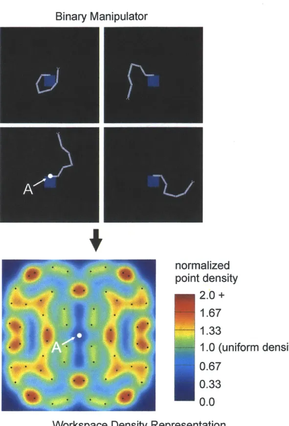
For optimization and design purposes, it is useful to view a discrete workspace cloud from the perspective of a density map. For a planar robot, a density map represents the density of points (the z-axis) versus the Cartesian location in space (the x- and y-axes). With a discrete cloud, the density map appears as spikes of infinite density at each workspace point, with all other areas of the map having a value of zero density (see top of Figure 2.2). To a designer, this density representation has little information and visual value other than to depict the cloud itself. However, if one applies a low-pass filter to the density map, the spikes blend together and provide a continuous approximation of the density of the workspace (see Figure 2.2). With this continuous approximation, one can more easily create metrics for the uniformity and distribution of the workspace cloud. Chapter 2. System-Level Planning, Analysis, and Simulation 23

(24)

Discrete Point Cloud

20 -II I 0 0 0 0 0 0 0 0 15 - 0 00 0 0s 0 0 0 0 0 0 0 0 0 0 0 -0 0 0 0 x oodiat norm0 0e 0 0 0 0 0

p72n densty

2. + 0 -)0 0 0

o

0 0 C1.6 0 0 0 0 5.0000 0 .13 -10 *s 0 1 1o is

x coordinate

normalized

point density

2.0+

1.67

1.33 1.0 (uniform density)

0.67

0.33

0.0 Continuous Density Representation

Figure 2.2. Transformation of a discrete point cloud to a continuous density representation using a low-pass (Gaussian) filter.

In the case studied here, the low-pass filter used was a spatial Gaussian filter, meaning that each point spike in the map was replaced by a bell-shaped peak that had the shape of a Gaussian (normal) distribution. The peak was normalized so that its height was exactly 1 unit, and the width of the peak (the standard deviation of the Gaussian) was

24

(25)

proportional to the square root of the workspace area divided by the total number of points. In this way, a uniformly distributed point cloud would have a continuous representation as a plateau of height 1 unit.

With a continuous density representation, one can quantify the uniformity of workspace distribution by taking the standard deviation of the z-values in the density map. A small standard deviation indicates a more uniform density distribution. This method for quantifying the distribution of the workspace can easily be extended to three-dimensional workspaces by adding a dimension to the density map. Information on the orientation of the workspace points can be included similarly by adding more dimensions to the density map. Of course this makes visualization of the map difficult, but nonetheless the notion of workspace distribution is still quantifiable.

Figure 2.3. A binary serial manipulator, showing the design variables li, 36, and (pi that can be

optimized to provide uniform workspace density.

With an optimization metric in place, an example case was studied to demonstrate the idea of optimizing a binary robot design to provide uniform workspace point density. For this case, a serial planar manipulator was examined, having between four and ten

binary actuators (see Figure 2.3). The joint angles are operated in binary fashion,

(26)

meaning they deflect an angle of ±pi from a nominal angle 60i. To be optimized were the lengths of each link, li, and the angles of deviation of each binary rotary joint, (pi. (In this example, 80i was set equal to zero for all i, but this variable also could have been optimized.) This robotic design results in a planar workspace composed of 2N points,

where N is the number of binary actuators.

A basic evolutionary algorithm was used to optimize the design variables of this design. This algorithm was not developed extensively, as it was used only to illustrate the idea of design optimization based on workspace qualities. The algorithm generated a random set of candidate designs and evaluated them based on their uniformity of workspace. It then selected the best candidates (those with the most uniform workspace densities) and mutated their variables by changing them slightly at random. This new generation of candidates was evaluated and compared to the previous generation. The best of the current and the previous generations were then kept and mutated again. The process was repeated hundreds of times until good solutions evolved. The result of one such optimization is shown in Figure 2.4. Note that the density map in this figure is much more uniform than the one shown in Figure 2.2. More sophisticated optimization methods could be developed to achieve faster convergence, and this would make an interesting study in the future.

(27)

Binary Manipulator

normalized

point density

j2

_2.0+

0 +

1.67

1.33 1.0 (uniform density)

-

0.67

0.33

0.0

Workspace Density Representation

Figure 2.4. A 6-DOF serial binary manipulator, optimizedfor uniform workspace density, showing afew binary configurations (top), and its workspace density map (bottom).

Chapter 2. System-Level Planning, Analysis, and Simulation

I

(28)

_____________________________________________________________ - -.. ~-.~

--2.3 Forward Kinematics

For binary robotic systems, it is sometimes convenient to formulate the forward kinematics using four-by-four homogeneous transformation matrices [Craig, 1989]. For example, the transformation matrix AoM describing the position and orientation of the end-effector relative to the base can be viewed as the product of the M intermediate transformations Aj.;, from module to module within the structure (see Figure 2.5). In other words,

M AOM = A01 A1,₂ ---. *AM -Im =

171

A.l

i=1

(2.1)

where M is the number of intermediate modules. This method of solution decomposes the kinematics of a complex structure into a series of smaller, simpler structures that are easier and faster to solve [Lees, Chirikjian, 1996].

ZM

xm

Figure 2.5. Coordinate frames

z

ZI

of each modulewithin a binary device.

Because of the discrete nature of binary devices, each term of the intermediate transformation Aj.2, can have only a finite number of possible values. If each module has Chapter 2. System-Level Planning, Analysis, and Simulation 28

(29)

only a few binary degrees of freedom, one can quickly enumerate all the values that the terms of A.u,i can possibly have. For example, if a module has three binary DOF, then

the module has 23 = 8 possible values for Ai~jj (notated by Ai.;j", Ai2) , ..., Ai.,! 8)). The

values can be computed once and stored into memory. Adding additional modules in a serial fashion will consequently increase the number of values stored in memory and thus memory requirements will grow linearly with an increasing number of modules [Lees, Chirikjian, 1996]. During run-time, forward kinematics computations need only know the binary state of the device to compute the transformation AoM using Equation 2.1.

The forward kinematic computations can be simplified further in the case of a robot with similar modules. If the robotic device is composed of identical modules, each

stage or module has the same kinematic characteristics and possesses the same values for Aj.7jM, Aj~j(2, ... , Aj~i~s). The number of computations performed and stored in memory

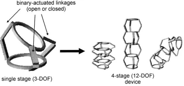
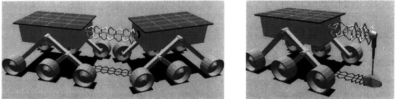
is consequently reduced by a factor of M, where M is the number of modules. One example of such a robot is the Binary Robotic Articulated Intelligent Device (BRAID), developed at the Field and Space Robotics Laboratory, which is a serial stack of identical parallel stages [Oropeza, 1999] (see Figures 2.6 and 2.7). Such a design could be used for manipulating instruments, collecting soil samples, or mating two cooperating robots, applications that require only moderate precision. See Appendix C for further discussion of the kinematics of the BRAID.

binary-actuated linkages (open or closed)

single stage (3-DO) 4-stage (12 DOF)

device

Figure 2.6 BRAID: a serial chain of binary-actuated parallel stages.

(30)

--.

Figure 2.7. Potential BRAID applications: (a) mating two rovers; (b) maneuvering an instrument.

One interesting aspect of binary robotic devices is that forward kinematics computations can be done without repeated use of computationally costly transcendental functions during run-time [Lees, Chirikjian, 1996]. Whereas continuous robots have infinite solution spaces requiring complex geometric calculations be performed during run-time, binary-actuated robot geometries can be computed offline ahead of time since there are only a finite number of states involved. The solution of the module kinematics (Ai-iji, Aj1,/2), ... , Aj.1js)) may of course require trigonometric or more complex

mathematics, but these need only be solved once, possibly on a different computer than the one being used for real-time control. During run-time, forward kinematic computations are trivial linear algebra (Equation 2.1) based on values stored in memory. No computationally costly mathematics are required at run-time. This computation can be implemented with even the most basic processing capabilities. In fact, even these computations can be performed offline; however with high-DOF systems the memory requirements for this can become quite large. For example, a five-stage BRAID can be viewed as five identical 3-DOF modules, requiring 16 x 2 = 128 floating point numbers of storage, or it can be viewed as one 15-DOF module, requiring 16 x 215 = 524,288 floating point numbers of storage.

2.4 Inverse Kinematics

Most strikingly different between continuous and binary-actuated robotic devices is the solution of their inverse kinematics. Instead of using geometric relations to

(31)

compute infinitely variable joint angles or link lengths, the inverse kinematics are solved by searching through the configuration space of the binary robot to find the configuration that minimizes error between target and end-effector position and orientation. There are many ways to search through this configuration space, and particular methods are often suited to particular applications [Ebert-Uphoff, et al, 1996; Chirikjian, 1997; Sujan, et al, 2001]. One goal of this study was to examine several inverse kinematic solution methods to determine those appropriate for implementation in applications.

In all the methods discussed below, the goal is to minimize some error value, which is a function of both the positional and orientational errors. In the cases studied here, this error value was defined as

total _ error = positional _ error 2 + Keror * angular _ error 2

1 (2.2)

fitness =

total _ error

where Kerror was a value around 100, angular error was specified in radians, and positional error was specified in percent of manipulator characteristic length (average of maximum and minimum possible lengths). Changing the value of Kerror simply shifts the

weighting between positional and angular errors. The basis for this cost function was made by imagining elastic elements between the desired and actual end-effector position; total error as defined here approximates the energy stored in the elastic elements due to the error. Thus the goal for the inverse kinematics solution methods is to minimize total

error (or maximize fitness).

2.4.1 Exhaustive Search

With modern computation speeds, an exhaustive search through the entire configuration space is possible for devices with low numbers of binary DOF. An exhaustive search algorithm typically computes the forward kinematics for the end-effector for each of the configurations, and stores this information in a look-up table in memory. At run-time, desired end-effector positions are compared to the information in Chapter 2. System-Level Planning, Analysis, and Simulation 31

(32)

the look-up table to determine the configuration that minimizes error. With an exhaustive search, the resulting solution is globally optimal, as the entire configuration space is searched; no potential solutions are overlooked.

The problem with exhaustive searches is that they are infeasible for high-DOF systems. This is because the search space grows exponentially with the number of actuators, each additional binary DOF doubling the size of the search space. A large search space takes a long time to search through and requires a great deal of memory. For example, a 10-DOF system requires the search through and storage of 210 = 1,024 states, while a 20-DOF system has 220 = 1,048,576 states. In this case a system with only

twice the physical complexity requires one thousand times the computation capability. In simulation studies, exhaustive searches were found to be quite effective for systems with less than fifteen DOF. Larger systems showed the exhaustive search to be too slow with modern computation for practical applications.

2.4.2 Combinatorial Search Algorithm

To deal with systems with larger numbers of binary actuators, a second algorithm was studied and compared to the exhaustive search method. This algorithm, denoted the

combinatorial search algorithm, solves the inverse kinematics by changing the state of

only a few actuators at a time [Lees, Chirikjian, 1996] (see Appendix A for example code). By limiting actuator state-changes to only a few at a time, rather than changing a large number of them all at once, the algorithm effectively reduces the search space to configurations that are close to the existing configuration in configuration space. This reduction in search space size over an exhaustive search is dramatic for high-DOF systems.

The first part of the search enumerates all the configurations that are within K actuator state-changes (bit-flips) of the current configuration, where K is a small number such as three. The algorithm then exhaustively searches these candidate configurations to find which one more closely matches the desired end-effector location. From this new configuration, the process is repeated to find an even better configuration. This process is repeated until a solution is converged upon. In this way, the combinatorial algorithm is Chapter 2. System-Level Planning, Analysis, and Simulation 32

(33)

like a steepest-descent optimization routine, since it reaches a minimum error by taking small steps (in configuration space) in the direction that most strongly reduces error. In simulations, the number of iterations to convergence was found to be of the order of N/3, where N is the number of DOF. The solution achieved with this algorithm is locally optimal; that is, there are no close configurations (in configuration space) that provide better results since all close configurations are exhaustively searched. While a globally optimal solution cannot be guaranteed like it can with the exhaustive search, for systems with many DOF the locally optimal solution was observed to be satisfactory for many

applications.

The increase in search speed with this algorithm over the exhaustive search can be shown mathematically by examining the size of the search space. For an exhaustive search, the size of the search space is the size of the entire configuration space, which is exactly 2N, where N is the number of binary DOF. With the combinatorial search

algorithm, the search space size is exactly

+...+ + [Lees, Chirikjian, 1996] (2.3)

K K - 1 0

where C is the number of iterations through the algorithm (order N/3), K is the number of bit-flips allowed per iteration, and the notation is the operator indicating the number

K

of K combinations among N objects (without regard to order), defined mathematically as

K (N - K).K! !(2.4)

Letting C N /3, substituting Equation 2.4 into 2.3, and collecting the highest order

terms, one can show that the search space size is of the order NK+J. With small K, this is a dramatically smaller search space than the exhaustive search when the number of DOF is large. Therefore the combinatorial search space experiences only polynomial growth

(34)

with increasing numbers of DOF, as opposed to the exponential growth experienced by an exhaustive search.

2.4.3 Genetic Algorithm

A genetic algorithm was a third search method studied for solving the inverse kinematics problem [Sujan, et al, 2001] (see Appendix B for example code). Genetic algorithms have been widely used to solve unusual or difficult optimization problems [Goldberg D, 1989]. A genetic algorithm is a stochastic optimization process that often succeeds when deterministic methods are impractical or impossible. In essence, a genetic algorithm generates a random population of candidate solutions and evolves out an optimal or near-optimal solution by evaluating, selecting, crossbreeding, and mutating the individuals within the population. Depending on the application, the manner in which these processes are carried out can range from quite simple to very complex. In simulations of binary robotic devices done here, a very basic genetic algorithm was sufficient to provide good results.

One aspect of binary robots that makes the genetic algorithm very natural and convenient lies in the binary nature of the robot itself. A prerequisite for using genetic algorithms is that the optimization variables must somehow be represented in a binary DNA-like manner, so that crossbreeding and mutation can be performed on candidate solutions. With many engineering problems, the conversion from the real-world problem to a binary encoding can be complicated. With the binary inverse kinematics problem, though, these complexities do not exist. The optimization problem is already formulated in a binary code.

With a genetic algorithm, the main algorithm design variables are the population size, the number of generations of evolution, the mutation factor (likelihood of bit mutation), the crossover ratio (fraction of the selected population that is cross-bred), crossover method (1-point, n-point, uniform, etc.), and the fitness metric used for evaluating individuals in the population. In this study, many of these algorithm variables were chosen heuristically based on rules of thumb or general performance of the algorithm. In simulations, ten separately evolved populations were used, with the final Chapter 2. System-Level Planning, Analysis, and Simulation 34

(35)

solution chosen from the best of all populations. Each of the ten populations had a size of one hundred individuals, and each population evolved over one hundred generations. These numbers were chosen because they gave reasonable performance and speed. For each new generation, a population of new individuals was selected based on the fitness of the individuals in the previous generation. The likelihood an individual was selected for the next generation was proportional to its fitness relative to the population (fitness being defined in Equation 2.2). This method of selection, the most common, is known as

proportional selection. The crossover ratio was set to 0.5, meaning half of the selected

population was crossbred, while the other half maintained its individuality. This ratio was recommended from literature as a good starting point for many applications [Goldberg D, 1989]. It provided good performance, and therefore was used. Uniform crossover was used to provide good diversity in populations (see Figure 2.8).

One-point

crossover Gene sequence is split in one place and

remainder is traded

Original genes Individual genes have

from two Uniform an equal probability of individuals crossover being kept or traded

Figure 2.8. Comparisons between basic crossover methods.

In terms of cross-over and mutations, some modifications to the basic genetic algorithm were made that improved performance of the algorithm. The kinematic structure that was used in simulation studies was that of the BRAID (see Figure 2.6). This device is composed of a serial chain of parallel stages. Each parallel stage has three binary DOF. By the nature of its structure, individual stages rather than individual bits Chapter 2. System-Level Planning, Analysis, and Simulation 35'

(36)

should be viewed as the essential building block of the device. The was seen to be more effective when working with the building blocks stages) rather than pieces of the building blocks (the individual bits). the algorithm performs crossover with two individuals, it swaps stages rather than individual bits between the individuals (see Figure 2.9).

Single bit crossover

genetic algorithm of the device (the Therefore, when (sets of three bits)

Original genes Stage (3-bit)

from two crossover

individuals

Figure 2.9. Stage crossover vs. bit crossover.

By the same reasoning, mutations were performed on stages rather than bits. In genetic algorithms, mutations provide random variations to individuals within the population, which helps ensure that the entire configuration space is represented. In this application, it appeared to be more effective to mutate stages (sets of three bits) rather than individual bits. The algorithm replaces the existing stage with one randomly chosen from the eight possible states the stage can have. While many phenomena of genetic algorithms are not easily explained, it is thought that the same reasoning used in the crossover discussion applies here; i.e. mutating the building blocks is more effective than mutating individual bits.

(37)

Comparing the genetic algorithm to the others discussed, the size of the search space explored by the genetic algorithm is given by

search _ space _size = E -G -P (2.5)

where E is the number of populations separately evolved (in this case 10), G is the number of generations for each population (100), and P is the number of individuals within the population (100). In studies done here, E, G, and P were kept constant relative to the number of degrees of freedom, N. For more advanced algorithm development, these values could be made a function of N, but this was not necessary for purposes here. The values of E, G, and P used here were found to be effective for systems having as many as 150 binary DOF. In the case of constant algorithm parameters, the search space size stays constant relative to the number of DOF. Within the algorithm, several computations take place that are linearly proportional to N (such as forward kinematics computations) and therefore computation time of the inverse kinematics using a genetic algorithm grows only linearly with the number of DOF of the system. As will be shown in the following section, this makes the genetic algorithm the fastest of those studied for systems having more than 40 DOF.

2.4.4 Algorithm Comparisons

Figure 2.10 shows the times for solving the inverse kinematics problem for each of the three algorithms described above. The times were computed from simulations based on the BRAID structure (see Figure 2.6), and were performed using a 600 MHz Pentium III processor. In these studies, the exhaustive search was observed to be the fastest for systems with less than 12 DOF, the combinatorial algorithm was the fastest for systems having between 12 and 40 DOF, and the genetic algorithm was the fastest for larger systems.

(38)

2 10 10 0 10 0 a) a) E -0 U) 10 10 10 -1 .3 14 10 -5 10

Inverse Kinematics Solution Time vs. Number of DOF (Pentium 1I1 600 MHz)

0 10 20 30

Number of DOF

40 50 60

Figure 2.10. Inverse kinematics solution times for various algorithms.

4.4.5 Error Analysis of Binary Systems

Errors in position and orientation for the various algorithms can be quantified on a stochastic basis using a Monte Carlo method. The inverse kinematics for one thousand random target points were solved for and the errors were recorded and quantified on a statistical basis. The targets were chosen from within a working workspace, which was defined as a region roughly 90% of the radius of the actual point cloud (see Figure 2.11). The working workspace represents the region in which actual tasks would be carried out, having sufficient point density to allow good performance. (It is assumed that the periphery of the true workspace has low point density.) Each target was given a random orientation. Again, computations were made from simulations of the BRAID structure. The specific BRAID geometry analyzed here was chosen by trial and error as one that had good motion properties by inspection.

Chapter 2. System-Level Planning, Analysis, and Simulation

--

p-e-exhaustive search

-F- combinatorial search genetic search

(39)

'4 ~14~ 1. *4 g 44 A . 'a.

Figure 2.11. Representative workspace of a 30-DOF BRAID. 1000 random target points were chosen from within the working workspace, a sphere whose size is slightly smaller than the actual

workspace cloud.

An example of the distribution of the errors is shown in Figure 2.12. These distributions are intended to give the designer an understanding for the size of errors encountered in binary systems and show that errors are not constant but still predictable statistically. For systems with 30 DOF (a ten-stage BRAID), displacement errors are generally within a few percent of the characteristic manipulator length and angular errors are within fifteen degrees. Such a system is unsuitable for precision work, but may be acceptable for such tasks as camera placement, crude instrument manipulation, and sample collection. For better angular precision (at the cost of displacement precision), one could simply increase the value of Kerror in the error cost function (Equation 2.2). One could also use a fine-motion stage to trim the errors involved with the binary system, although this was not a focus of this study. The shapes of the error distributions are very

Concept development for lightweight binary-actuated robotic devices, with application to space systems

JUL 16 2001

ACKNOWLEDGEMENTS

CONTENTS

FIGURES

INTRODUCTION

1.1 Introduction

1.2 Motivation

1.3 The Self-Transforming Explorer (STX) Concept

1.3.2 Polymer-Based Compliant Mechanisms

1.3.3 Binary Actuation and Control

1.3.4 Bistable Joints and Structures

1.4 Background and Literature Review

1.5

Research Overview

1.6 Thesis Outline

2

SYSTEM-LEVEL PLANNING, ANALYSIS, AND

SIMULATION

2.1 Introduction

2.2

Workspace Optimization

Discrete Point Cloud

p72n densty

o

x coordinate

normalized

point density

2.0+

1.67

1.33

1.0 (uniform density)

0.67

0.33

0.0

Continuous Density Representation

Binary Manipulator

normalized

point density

j2

2.0+

0 +

1.67

1.33

1.0 (uniform density)

-

-

0.67

0.33

Workspace Density Representation

I

--2.3 Forward Kinematics

171

2.4 Inverse Kinematics

2.4.1 Exhaustive Search

2.4.2

Combinatorial Search Algorithm

2.4.3 Genetic Algorithm

2.4.4 Algorithm Comparisons

4.4.5

Error Analysis of Binary Systems

_2.0+