A comparison of electric and hydraulic approaches to fluid flow simulation and hydraulic parameters inversion

A Comparison of Electric and Hydraulic Approaches

to Fluid Flow Simulation and Hydraulic Parameters

Inversion

by

Saleh Mohammed Al Nasser

Submitted to the Department of Earth Atmospheric and Planetary

Sciences

in partial fulfillment of the requirements for the degree of

Master of Science

at the

MASSACHUSETTS INSTITUTE OF TECHNOLOGY

September 2016

Massachusetts Institute of Technology 2016. All rights reserved.

MASSAHUSETTS INSTITUTE_MS-OF TECHNOLOGY

SEP

19 2016

LIBRARIES

ARCHIVES

Author ...

Certified by.

Signature redacted

Department of Earth Atmospheric and Planetary Sciences

1-August-2016

Signature redacted

I

Accepted by ..

Frank Dale Morgan

Professor of Geophysics

Thesis Supervisor

Signature redacted

Robert D. Van der Hilst

Schlumberger Professor of Earth Sciences,

Head of the Department of Earth, Atmospheric, and Planetary Sciences

A Comparison of Electric and Hydraulic Approaches to Fluid

Flow Simulation and Hydraulic Parameters Inversion

by

Saleh Mohammed Al Nasser

Submitted to the Department of Earth Atmospheric and Planetary Sciences on 1-August-2016, in partial fulfillment of the

requirements for the degree of Master of Science

Abstract

History matching and prediction of future performance of hydrocarbon reservoirs and groundwater aquifers are considered some of the biggest challenges facing hydrol-ogists and petroleum engineers. The complexity of the simulation method, in addition to the huge amount of input data, makes evaluating the reservoir performance expen-sive. The conventional reservoir history matching procedure usually requires a trial and error process of altering various reservoir parameters and simulating the pressure distribution and field production, or what is known as 'Forward Modeling'. In this study, I propose the use of regular electrical arrays to simulate aquifer drawdowns. By representing reservoir hydraulic conductivities as electric resistors and storativities as capacitors, simulating the potential response gives results similar to that of solving the hydraulic flow equations. Scaling the electrical parameters results in an equiva-lent approximation of voltage and hydraulic head. A set of synthetic aquifer models with increasing structure complexity were simulated under the Dupuit-Fochheimer assumption of negligible vertical flow. Under the finite difference scheme, aquifers subjected to a constant pumping rate were modeled under different boundary condi-tions. The transient drawdown data curves from either a single well or multiple wells were obtained, and the reservoir data were inverted for the hydraulic parameters. Be-cause both electrical and hydraulic approaches result in similar response, parameters inversion can be performed on either system. Consequently, the hydraulic equations were used in the inversion. Inversion was performed according to the method of damped least-square where the Jacobian matrix is decomposed by Singular Value Decomposition (SVD). Furthermore, hydraulic aquifers are attempted to be modeled with a binary conductivity structure, which is an effective medium of two hydraulic conductivities.

Thesis Supervisor: Frank Dale Morgan Title: Professor of Geophysics

3

Acknowledgments

I would like to convey my gratitude an appreciation to my thesis advisor, Prof.

Frank Dale Morgan. His continuous support and care is beyond measure. Dale treated

me like a son of his, and kept pushing me into further learning and experimenting.

The door to his office is always open, whenever I need an academic or personal advises.

I owe him a huge respect for the person I changed to in the past two years.

My appreciation is extended to my thesis committee members, Prof. Navi Toksoz,

Dr. Daniel Burns and Dr. Michael Fehler. Each one of them has influenced me in

their unique ways. I have set so many times in Nafi's office listening to his wisdom

thoughts and ideas. I am deeply thankful to Dan for his continuous encouragement,

and informative discussions. Dan has a special way to forcefully put a smile on my

face. Mike always helped me seeing issues and problems from different perspective.

His creative thoughts helped me a lot during my stay at MIT.

I would also like to thank and acknowledge the professors who taught me at MIT;

Rob van der Hilst, Tom Herring, Bradford Hager, Allison Malcolm, Ruben Juanes

and others.

I would like to acknowledge my colleagues at EAPS and ERL for their support

and kindness. Each one has given me a lot of his or her time and effort. Thanks to

EAPS and ERL administrations for all the help they provided.

I would like to thank Saudi Aramco for the full scholarship and financial support.

My thanks are extended to the members of Geophysical Technology Team at EXPEC

ARC, especially to Dr. Panos Kelamis for his believe in me.

My deepest appreciation and gratitude to my parents ( Mohammed Al Nasser &

Fahima Al Shilaty) and my siblings for the limitless love and care. My only hope is

to make them proud. This work is dedicated to loved ones who I lost and contributed

a lot in the development of my life.

Contents

1 Introduction 17

1.1 O bjective . . . . 18

1.2 Literature Review . . . . 18

2 Hydraulic Modeling 21 2.1 General Fluid Flow Equations in Porous Media . . . . 21

2.2 Discretization of the Fluid Flow Equation . . . . 23

2.2.1 2-D Finite Volume . . . . 23

2.2.2 2-D Finite Difference and Forward Modeling . . . . 26

3 Electrical Analogy 33 3.1 Resistance-Capacitance Transient Simulation . . . . 35

3.1.1 ID RC Circuits . . . . 35

3.1.2 2-D RC Circuits . . . . 39

3.2 Comparing 2-D Electrical and Hydraulic Approaches in Fluid Flow . 41 4 Inversion 55 4.1 T heory . . . . 55

4.2 Results In (x,y) Coordinates . . . . 57

4.2.1 Case 1: Simple Confined Aquifer . . . . 58

4.2.2 Case 2: Simple Unconfined Aquifer . . . . 64

4.2.3 Case 3: Complex Confined Aquifer . . . . 67

4.2.4 Case

4:

7

4.3 Results In

(x,z)

Coordinates . . . .

82

4.3.1

Case 1:

Simple Model . . . .

82

4.3.2

Case 2:

Reduced Inversion Structure of a Complex Model

85

4.4

Improved Binary Model . . . .

86

5

91

5.1 Discussion . . . .

91

5.2 Conclusion . . . .

93

5.3 Future Work . . . .

95

List of Figures

2-1 Mass conservation in a unit block (Wang & Anderson, 1982) . . . . . 22

2-2 Finite-Volume discretization of a two-dimensional, horizontal flow. . . 24

2-3 Transmissibility distribution on grid. . . . . 25

2-4 Schematic of a 1-D aquifer showing the the boundary and initial con-ditions. . . . . 27

2-5 Head change over a distance at two different times. The solid lines are the finite difference solution while the dots are the analytical solution. 28 2-6 Change of head across 100 m distance after 1,000 minutes. The solid lines are the finite difference solution while the dots are the analytical solution of the unconfined steady-state equation. . . . . 30

3-1 Porous Medium Unit. . . . . 34

3-2 Simple resistor-capacitor circuit. . . . . 34

3-3 Simple RC lump model . . . . 36

3-4 2-D Electrical network. . . . . 39

3-5 Schematic of the aquifer above an impermeable layer. The aquifer dimensions are 1, 000m x1, 000m. The initial head hi is 100m. Dirichlet boundaries are represented by specific head h, equal to 100m.

Q

3-6 a) Hydraulic conductivity in (x, y). The well location is represented by a white dot. b) The head distribution in plan view after 500 days of pumping. c) Head change with time at the well location. d) Evolution of head across the aquifer marked by the dashed line on figure b. . . 42

3-7 3 x 3 RC circuit that has a constant voltage source on all sides and

current output at the center.

. . . .

43

3-8

The solid line is the the result of the hydraulic finite difference solution.

The red dots are the result of the RC simulation. Voltage was scaled

to head using the scaling factors equal to 1.

. . . .

44

3-9 The percent difference between the RC and hydraulic approaches.

45

3-10 Schematic of the aquifer. The dimension of the aquifer is 1, OOm x

1, 000m. The initial hi is 100m. Dirichlet boundaries are represented

by specific h equal to 100m at east and north boundaries.

Q

is the

constant discharge rate. The rest of the boundaries are no flow. . . . 46

3-11 a) Hydraulic conductivity in (x, y) coordinates. b) The head

distribu-tion in plan view after 500 days of pumping. c) Transient head response

at the well location. d) Evolution of head across the aquifer marked

by the dashed line on figure b. . . . .

47

3-12 The solid line is the finite difference solution of the fluid equations.

The dots are the result of RC simulation. . . . .

48

3-13 The percent difference between the RC and hydraulic approaches for

the second example . . . .

49

3-14 Schematic of the aquifer. The bottom is an impermeable boundary.

The dimension of the aquifer is 1000m x 1000m. The initial h is 100m.

Dirichlet boundaries are represented by specific h equal to 100m at the

four boundaries.

Q

is the constant discharge rate. . . . .

50

3-15 a) Hydraulic conductivity in (x, y) coordinates. b) The head

distri-bution in plan view after 500 days of pumping. c) Head change with

time at the well location. d) Time evolution of head across the aquifer

marked by dashed line on figure (b). . . . .

51

3-16 The solid line is the groundwater finite difference solution. The dots

are the result of the RC simulation. . . . .

52

3-18 The difference in CPU time for solving the two systems (hydraulic and RC) using a finite difference method. . . . . 54

4-1 The main steps of the Inversion method. . . . . 56

4-2 a) Is the hydraulic conductivity model. The color bar is an indication of the transmissivity value. Red dots represents the locations of the observation wells, and the black point is the location of the pumping well. b) is the head data from the 121 wells. . . . . 59

4-3 a) and b) The true model and the inverted model, respectively. c) RMSE plotted against iteration number. d) The head difference be-tween the data and the inversion results at each well, in percentage R M SE . . . . 60

4-4 _{a) and b) The true model and the inverted model, respectively. c)} The value of the RMSE plotted against iteration number. d) The head difference between the data and the inversion results at each well, in percentage RM SE. . . . . 61

4-5 a) and b) The true model and the inverted model, respectively. c) Smoothed inverted model. d) The head difference between the data and the inversion results at each well, in percentage RMSE. . . . . . 62

4-6 a) and b) The true model and the inverted model, respectively. c) A smoothed image of the inverted model. d) The head difference between the data and the inversion results at each well in percentage RMSE. 63

4-7 a) The hydraulic conductivity model. Red dots are the location of the observation wells and the black point is the location of the pumping well. b) The head data from the 121 wells. . . . . 64

4-8 (a) and (b) The true model and the inverted model. c) The value of the RMSE plotted against iteration number. d) illustrates the head difference between the data and the inversion results at each well, in percentage RM SE. . . . . 65

11

4-9 a) and b) The true model and the inverted model, respectively. The

number of observation wells is reduced. c) Smoothed image of the

inverted model. d) illustrates the head difference between the data

and the inversion results at each well, in percentage RMSE . . . .

66

4-10 a) Hydraulic conductivity model. Red dots are the locations of the

observation wells and the black dot is the location of the pumping

well. b) The head data from the 121 wells.

. . . .

67

4-11 (a) and (b) The true model and smoothed inverted model. The number

of observation wells is reduced. c) RMSE plotted against iteration

number. d) The head difference between the data and the inversion

results at each well, in percentage RMSE.

. . . .

68

4-12 a) Hydraulic conductivity model. The red dots represent the

loca-tions of the observation wells, and the black dot is the location of the

pumping well. b) head data from the 121 wells. . . . .

69

4-13 a) and b) The true model and a the smoothed inverted image,

re-spectively. c) RMSE plotted against iteration number. d) The head

difference between the data and the inversion results at each well, in

percentage RM SE.

. . . .

70

4-14 a) Hydraulic conductivity model. Red dot are the location of the

ob-servation wells and the black point is the location of the pumping well.

b) head data from the 121 wells.

. . . .

71

4-15 (a) and (b) The true model and the inverted model c) The value of

the RMSE plotted against iteration number. d) The head difference

between the data and the inversion results at each well in percentage

R M SE . . . .

72

4-16 A histogram showing the distribution of inverted parameters. The

black line in the middle is where the data is split to create the binary

m odel.

. . . .

74

4-17 a) The binary model. b) Transient head of true model and binary model at an arbitrary well. c) is the difference in percentage between binary and true head responses. . . . . 75 4-18 a) The true model. b) the inverted model. c) A smoothed inverted

image. d) The head difference between the data and the inversion results at each well in percentage RMSE. . . . . 77

4-19 a) The binary model. b) Non-steady head response at the production well from modeling the true model, inverted model and binary model. c) The difference in percentage between the curves . . . . . 78 4-20 a)An averaged transmissivity model. b) A smoothed averaged model. 79 4-21 The three curves represent the transient head from true, binary,

inver-sion and averaged models. . . . . 80 4-22 The percent difference between true head and inverted head in (red).

The difference between the true head and binary model is in (blue) and the (yellow) curve is the percent difference between the true model and the averaged m odel. . . . . 81 4-23 (a) and (b) are the true model and the inverted model. Observation

wells are in white, and production well is drawn in red. The red dots are the locations where head measurements are collected. The black dot is the location where the production well is screened. c) The value of the RMSE plotted against iteration number. d) Illustrates the head difference between the data and the inversion results at each measure-ment point in percentage RMSE. . . . . 83

4-24 a) The true model b) The inverted model. Observation wells are in white, and production well is drawn in red. The red dots are the locations where head measurements are collected. The black dot is the location where the production well is screened. c) A smooth image of the inversion result. d) The head difference between the data and the inversion results at each measurement point in percentage RMSE. . . 84

4-25 a) The true model b) The inverted model. True model has 55 x 55cells,

and inverted model is 11 x 11. Observation wells are in white, and

production well is drawn in red. The red dots are the locations where

head measurements are collected. The black dot is the location where

the production well is screened. c) A smoothed version of the inverted

image. d) The head difference between the data and the inversion

results at each measurement point in percentage RMSE.

. . . .

85

4-26 a)The binary model. b) Transient head of true model, inverted model

and binary model at the production well. c) The difference in

percent-age between the curves.

. . . .

86

4-27 A histogram showing the distribution of inverted parameters. The

black line in the middle is where the data is initially split at an arbitrary

location to create the binary model.

. . . .

87

4-28 The main steps in choosing the improved binary model. First,

pa-rameter distribution is split and two averages computed. Second, the

binary model is used in the forward model. Third, binary results are

compared to true data. Steps are repeated with different split points

until an improved fit is achieved.

. . . .

88

4-29 a)The optimum binary model created by the geometric mean averaging.

b) Transient head of true model, inverted model and binary model

at the production well. c) The difference in percentage between the

curves.

. . . .

89

4-30 a)The optimum binary model created by the arithmetic mean

aver-aging. b) Transient head of true model, inverted model and binary

model at the production well. c) The difference in percentage between

the curves. ...

...

90

5-1 A true model which was computed with 104 was reduced to 102 and resulted in good fit to the true data. From the inverted image a binary model was created and still resulted in a good fit to true data. The future work will involve the inversion of the 3-D reservoirs. . . . . . 94

Chapter 1

Introduction

If you are working in either groundwater hydrology or the petroleum engineering

industry, your optimal objective is to manage reservoirs in an accurate, fast, and cost-effective manner. This is a challenging task that requires a good understand-ing of a given reservoir's geology and the physics of fluid flow. This means that an accurate numerical simulator must be developed to describe the fundamental flow equations with sufficient accuracy. Advances in computer power facilitate large-scale simulations of aquifers and reservoirs. However, the required time and cost for sim-ulation is proportional to the complexity of the reservoir's structure and size. Many numerical techniques have been used to simulate fluid flow, including: finite differ-ence, finite element, and finite volume. Using such numerical schemes yield many advantages and disadvantages. Alternatively, electrical analog computers have been implemented for history matching and forecasting the reservoir performance (Bruce, 1942). Previously, the lack of high-performance digital computers made implementing the electrical analog for simulation purposes advantageous. Regardless of the method used, the main objective is to map the heterogeneity of the reservoir in a sufficiently accurate manner. Nowdays there are so much 3-D and 2-D 'Forward Modeling' in flow systems. In this study, We attempt to prove that these expensive modeling are unnecessary to model hydraulic or petroleum reservoirs.

1.1

Objective

This study has two main objectives. The first objective is to compare two ap-proaches to simulating the non-steady fluid system. A set of forward modeling scenarios will be simulated by solving the flow equation using the finite difference scheme. The alternative solution is to simulate the aquifer by an electrical Resistance-Capacitance (RC) network.

Secondly, an inversion scheme is developed to estimate a reduced-flow structure of confined and unconfined aquifers. A reduced-flow structure is referred to an effective

'coarse scale' model that gives same flow as a fine scale model. The two main pa-rameters defining the flow structure are, hydraulic conductivity or transmissivity and storativity. The conductivity or transmissivity describes the fluid conducting prop-erties of the porous medium, and storativity describes the fluid storing propprop-erties of the porous medium (Lebbe, 2012). Producing a model that agrees with the observed data in a short time but still having great accuracy is the second objective. Inversion is performed on 2-dimensional aquifers. Results of inversions are presented for two different bases; (X, y) and (x, z).

1.2

Literature Review

Various studies have been conducted on simulating groundwater hydrology using electrical analog computers. Multiple attempts were made in simulating confined and unconfined aquifers as well. The analog network is a set of resistors and capacitors that are scaled either up or down to represent aquifer's parameters (Walton, 1964). A three-dimensional approach to simulate steady state flow to wells in unconfined aquifers was introduced by Stallman (1963). Studies have been also done on de-termining the permeability of an aquifer using electrical analog models ( Mundorff, 1972). Groundwater modeling can be automated to produce an accurate estimation of the aquifer parameters. However, factors such as heterogeneity, time, sensitivity, and uncertainty make system inversion difficult (Carrera, 2004). One of the earliest

works in determining the physical properties of aquifers was done based on the flow net approach by Bennet and Meyer (1952). However, Stallman (1956) was the first to solve the problem using electrical analog computers. He manages to estimate the dis-tribution of transmissivities by interpolating head values over finite difference grids. Another approach was attempted by Nelson (1960 and 1961), where he solved the inverse problem for steady state systems. His conclusion stated that the knowledge

of the fluid fluxes with the head values are important in determining transmissivities. Bruce (1942) invented an apparatus that simulated oil-reservoir behavior. Jacquard and Jain (1965) were the first to apply least squares to invert for the permeability of petroleum reservoirs. They divided the reservoir into zones of constant perme-ability and used least squares to minimize the sum of squared residuals. However, my approach attempts to invert for a simpler and reduced parameter structure of aquifers. Neuman (1972) developed an analytical or type curves solution to estimate conductivity of homogeneous unconfined aquifers. In addition, multiple studies were done on solving the problem using other techniques such as slug tests, geophysical measurements and borehole flowmeters (Copper et al. 1967, Dagan 1978, Darnet et al. 2003, Crisman et all. 2007). This study proceeds to invert for the hydraulic conductivities or transmissivities of aquifers through damped least-square solutions using Singular Value Decomposition (SVD). Ekinci (2008) implemented this inversion on 1-D resistivity sounding systems. Furthermore, an attempt to reduce an aquifer's structure is achieved through using the concept of a binary model. The approach of binary model appeared in the segmentation of digital images ( lie et al, 2004). I am going to use the same concept to represent the aquifer with binary conductivity structure.

Chapter 2

Hydraulic Modeling

To achieve the primary objectives of this study, a good understanding of fluid flow in porous media is required. In this chapter, the basic derivation to the general fluid flow equations are explained along with their numerical solutions.

2.1

General Fluid Flow Equations in Porous Media

Deriving the fluid flow equation in porous media must take the law of mass con-servation into account. It requires that there be no net change in the mass of the fluid-contained reservoir volume. Any change in the fluid mass exiting the volume of the reservoir must be balanced by a mass flux into the volume.

Figure 2.1 illustrates a small cube of dimensions dx, dy and dz representing an infinitesimal volume of the reservoir. The governing equation of mass conservation can be represented as;

flow in - flow out = mass accumulation. flow in = pUxdydz + pUydxdz + pUzdxdy.

flow out= p(Ux+ udx)dydz + p(Uy + Idy)dxdz + p(Uz

+

mass accumulation Mf 9 (p4dxdydz).

rt pt

where

U

I ,d Jdxdy IN.,>

~j

Figure 2-1: Mass conservation in a unit block (Wang & Anderson, 1982)

With a little algebra, the following equation can be derived:

+

at

For a slightly compressible fluid, Eq(2.1) can be written as,

($Cf + Cr) +V -U = o. at and U =

--

where Cf is the fluid compressibility, C, is the rock compressibility, P is pressure, K is hydraulic conductivity, y is the fluid viscosity, and g the gravitational acceleration.

If fluid is considered to be of constant density, the change in pressure is related to the change in head (h) through the following equation (Delleur, 1999):

OP

ah

at= pg.

at

at

.1

Thus, the fluid flow equation can be written as

Oh

pg(qCf + C,)

t= V -(K -Vh).

(2.5)

where K is the hydraulic conductivity.

If a specific storage coefficient (Gorelick, Freeze, Donohue and Keely, 1993) is introduced and defined as:

SS= pg(bCf +

Cr).

Eq(2.5) can also be expressed as:

Oh

SS -

= V - (K -Vh).

(2.7)

at

2.2

Discretization of the Fluid Flow Equation

This section demonstrates the numerical solution of the flow equation and explains two different methods: the finite volume and finite difference. Most of the simulations presented in this study are approached through finite difference.

2.2.1

2-D Finite Volume

To discretize Eq(2.7) using finite volumes, it must be written in integral form using a single cell Q. If flux U is defined by (K - Vh), then

[S

a

+

V -U]dQ.

(2.8)

ag

t

which can be written as:

Ss

j

d +

U -ndR.

(2.9)

at f i IR

where R is the surface of the control volume and n represents the unit vector normal to the surface.

The surface integral can be calculated by summing the integrals over the faces of 23

y

axis

UY

x axis

Figure 2-2: Finite-Volume discretization of a two-dimensional, horizontal flow.

the cell (i, j) Oh

S,-Sxcty +

at

+

1 *

(-1)dR

+

Considering the two-point flux approximation (TPFA) (Lie, 2015), the integral of the fluid flux across each face of the cell can be written as:

i

_I7

U__ (-1)dR+ U

-(+1)dR

U - (+1)dR].

(2.10) R

_I+7

y axis

T'T_IT

x axis Figure 2-3: Transmissibility distribution on grid.

where T. 1 . is the transmissibility, which is equivalent to the conductivity K

multi-plied by the thickness of the aquifer. on the east side of the cell.

Thus, the final discritization of the fluid flow equation of the cell (i, J) is:

S

- T

which can be written in matrix form such that:

(C +

OT)hn+

(C

-

(1

-

9)T)h"n

+ b.

where C is a diagonal matrix of size (Nx x Ny, Nx x Ny) and T is a matrix of size (Nx x Ny, Nx x Ny) that has a main diagonal vector and two upper and lower

sub-diagonal vectors. hn+1 and 1h" are column vectors of pressure, where n and n + 1

are the current and future time steps. The column vector b represents the boundary values.

25

10.) - T _{1] 1- i,} hn+1 _i-1, TY _{ij- 1 ' "ij-.!}1 n+ I

2 2 2

2.2.2

2-D Finite Difference and Forward Modeling

Several models were computed to represent the synthetic data. The forward mod-eling examples cover both confined and unconfined aquifers. In both types, the reser-voirs vary from homogeneous to heterogeneous in structure. This section defines the two aquifer types and lays out the second order central difference finite difference solution for each type.

Confined Aquifers

A confined aquifer is defined as a pressure aquifer that is bounded by impervious layers from the top and the bottom. The general 2-D fluid flow equation for a confined aquifer is:

92

h

h

KxB + K B_ = S-- R. (2.14)

a2X y 2y

at

where R is the volume of recharge-per-unit time per unit aquifer area and B is the thickness of the aquifer. The 1-D analytical solution of Eq(2.14) can be expressed as (Wand and Anderson, 1982):

(h2-- hi)x 2

'

h(x, t) = hi + + - E sin( )e- -SIT (2.15)

S 7n=1 n

where h, and h2 are boundary head values at the two sides of the aquifers. 1 is the

total length of the aquifer.

The finite difference approximation to Eq (2.14) is:

S

Y(h

-

+ (T " + TY _ + T:+I'j + TY )h' (2.16)

+T i hn+1_Tx h?-+l T" _hn+1

+ Q

₀

the scheme, we compare the finite difference solution to the analytical solution (Eq (2.15)). Both solutions were computed for a homogeneous, one-dimensional (100 -meter) aquifer, that is 10m thick. The head is set at constant rate at the right and left boundaries. The left boundary is at 16m head value and the right is at 11m. The initial head across the model is 16m. The hydraulic conductivity is constant everywhere at a value of K = 0.002m/day. The storativity is S = 0.02. Aquifer thickness is B =

lOn.

h

=16m

x=0

T

B=1Om

I

x=1=100

h

=11m

Figure 2-4: Schematic of a 1-D aquifer showing the the boundary and initial condi-tions.

Details about the 2-D simulation examples are presented in Chapter 3.

27

13 12.5

10

Finite Difference Solution

& Analytical Solution

FD @500 min -FD @rP 100 min . Analytical solution * Analytical Solution 20 30 40 50 60 70 80 90 Distance (N)

Figure 2-5: Head change over a distanee at two different times. The solid liines are the finite difference solution while the dots are the analytical solution.

16 15. ' 14.5

E

Unconfined Aquifers

An unconfined aquifer is often defined as a water table aquifer that exists below the surface. The top of the aquifer is subjected to recharge, and its water table acts as the upper boundary. The general 2-dimensional groundwater flow equation for an unconfined aquifer is:

K

It2

h

Oh

KS + KY = S -R. (2.17)

a2X . jg2y at

The 1-D steady-state solution of Eq (2.17) can be expressed analyticaly by:

(h

h

I 2 2 -

+

11

The implicit finite difference approximation of Eq(2.17) is expressed as:

hn+1 - hn+1 hn+1 - hn+1 1 1-1, j

+

hj-

h.

h'j

h+

h)

Q

6t

6x~y

2

13

2

We again compare the finite difference solution to the analytical solution to confirm the method's accuracy. Figure 2-6 presents the comparison between the two solutions. Both solutions were computed for a homogeneous, 100m, 1-D unconfined aquifer. Left and right head boundaries are set at constant values 16m and 11m. The initial head across the model is 16m. The hydraulic conductivity is constant everywhere at a

value of K = 0.002m/day. The storativity is S = 0.02. The aquifer thickness is

represented by the level of the water table.

Finite Difference and Analytical Solution for Unconfined Aquifer

20 30 40 50

Distance (m)

60 70 80 90

Figure 2-6: Change of head across 100 in distance after 1,000 minutes. The solid liles are the finite difference solution while the (lots are the analytical solution of the unconfined steady-state equation.

16 15 15 4.5 14 E FD * Analytical -13.5 13 12,5 12 11.5 C I I I - -5 4 1

Boundary Conditions

Boundary and initial conditions are required to solve the transient flow equations. Two types of boundaries can be applied to the aquifer simulation:

-Dirichlet Boundary Condition exists when the head on the aquifer boundary is specified.

-Neumann Boundary Condition occurs when the flux on the aquifer boundary is specified.

Chapter 3

Electrical Analogy

Consider a single block in the reservoir Figure 3-1. The material balance law

requires that the mass of fluid exiting the block minus the fluid entering the block is balanced by the change in density (p) times the fluid volume (Vo). This can be expressed as

dp

Mass, - Mass2 = V0 -. (3.1)

dt

Knowing Darcy's law, which can be expressed as

Mass Ah

Q

p

L

where

Q

of the block in m, and K is hydraulic conductivity in m/day. The material balance equation may be written as:

V$S d p

Q1

p dt'

hi - h2 =

Q.

KA

Now consider the circuit in the Figure 3-2 . Ohm's law can be expressed as:

(V1 - V2)

=

Ri.

(3.5)

where V is voltage and i is the electric current.

Figure 3-1: Porous Medium Unit.

R I(

Figure 3-2: Simple resistor-capacitor circuit.

From this equation, we can see the similarity with Eq(3.4). If the head i is

equiv-alent to voltage V, and the volume flow rate is equivequiv-alent to current i in the electric circuit,, then the electric resistance R can be set equivalent to the fluid resistance expression, such that:

L

KA (3.6)

The value of the electric capacitance can then be found in comparing the following equations:

QC

Q1

OV i1 - 2 = C .t

Thus, it can be inferred that the electric capacitance is:

C = ASN. 34 (3.7) (3.8) (3.9) C

where A and S, are the area and specific storage, Scaling the hydraulic units to the analogous factors (Bermes, 1969):

O

=

fQ.

h

V-Q

electrical units is done with four

(3.10)

(3.11)

(3.12)

(3.13)

where 0 is in m3_,

Q

in coulombs, h in meters, V in volts,

Q

td is time in days and t, is time in seconds. Thus, the units of the four factors are as

follows:

fI

/coulombs,

f

m/volts,

f

/day/amps

f4

The relation between the factors is as follows:

f3f 1. The

relation

(3.14)

scaling factors are chosen to be equal to one in this study to simplify the between the electrical and hydraulic units.

3.1

Resistance- Capacitance Transient Simulation

The electrical analog model is a regular network of resistors and capacitors. As explained earlier, resistors are inversely proportional to the aquifer's hydraulic con-ductivity, and capacitance is represented by the storativity of the aquifer. In this section, the solution for single RC-lumped model (Michael,1999) is derived. This is considered as the basis of the 2-D RC analog network.

3.1.1

1D RC Circuits

If the circuit in Figure 3-3 is considered and Kirchhoff's Current Law (KCL) is applied at node VCi, then we can write:

)

C1 C2

T

T

Figure 3-3: Simple RC lump model

VCi -

V

R1, + C1 dc + Vc

dt

Then, applying Kirchhoff's Current Law (KCL) at node VC2, we obtain

VC2 - VCi

+ C2 = 0.

dt

Equation (3.15) and Eq (3.16) can be expressed in matrix form:

1 1 1 1

C1 R1+

R

C

R

C

R

C

If matrix A is defined to be equal to the following,

1 C1l 1

R

R

_

dvc1

dt

dt

(3.17)

then,

dvC

dt

dt

Vs

R

C

0

We are interested in finding functions vc1 (t) and VC2 (t), which satisfy the above

matrix. The voltage across the capacitors can be expressed as the sum of a transient part that depends on t, and a steady-state solution that is reached as t -+ oc.

In the steady-state case, the voltages across C1 and C2 are constant. Because vc1 and VC₂ are constant, we can write

dvc

= 0.

dt

dt

Substitution of these expressions in the matrix results in the following:

vC1 = VC₂ = VS.

Based on the knowledge of the first-order differential equation of a simple RC circuit, we can assume the transient solution is of the form:

voC = vile I

+

VC2 = v21e81t + v2 2es2t

(3.18)

(3.19)

si and s2 are the natural frequencies of the circuit. We can determine the values of si and s2 from the eigenvalues of matrix A.

We can rewrite Eq (3.18) and Eq (3.19) in term of eigenvectors, such that: 37

VC1 X11 X21

= CesIt + Des2t . (3.20)

VC2X1X2

X1 1 X21

where and are the two eigenvectors of matrix A.

X12 X2 2

However, values of the constants C and D have to be determined to obtain the com-plete solution of all VC values. This is achieved by knowing the initial conditions of the system. We can find C and D through the following formula:

C

(3.21)

VY₊₁

VX

Rx

C

Figure 3-4: 2-D Electrical network.

3.1.2

2-D RC Circuits

Let us consider a 3 x 3 RC circuit as shown in Figure 3-4. Each node is rep-resented by one capacitor and four resistors. The capacitors are connected to the ground. The circuit boundaries are connected to voltage sources, which represent the reservoir boundaries. Applying Kirchhoff's current law at each node will result in nine deferential equations. The middle node can be expressed as:

dVc

I

_d+

₊

₁₊

Y

_Vi

_-Vc(RH

Y

V

V1

1

+ (3.22)

dt C Rt 1 R i R ix fRm lok lik

Writing the equations in a matrix form looks like 39

dVj

dt

dVc

dt

dI

VC-

~0

0

.

dt

dt

b

d

b

exiting the center cell. By following the same procedure as in the 1-D example, a distribution of the voltages at each node can be estimated.

Vj-3.2

Comparing 2-D Electrical and Hydraulic Approaches

in Fluid Flow

In this section, 2-D forward solution by hydraulic and electrical methods are

compared. These models are compared with the modeled transient solution of

2-D Resistance-Capacitance (RC) circuits. The groundwater flow equations are solved

in the (x., y) coordinates using a finite difference scheme. The vertical flow is ignored.

The first example simulates a confined aquifer with uniform thickness, (see

Fig-ure 3-5). The initial head 11 is constant in the (x., y) plane. Dirichlet-type boundary

conditions are implemented on all boundaries with specified head values h at the four

boundaries. For simplicity, the aquifer is homogeneous with uniform hydraulic con-ductivity everywhere. To simulate the transient change in the head, fluid is pumped at a constant flow rate fron the center of the model. Given, the boundary conditions. hydraulic conductivity, and discharge rate, the flow Eq 2-14 can be solved.

Figure 3-5 is a, schematic representation of the aquifer. The model is subdivided

to 51 x 51 cells with dx dy 19.6m. The result of the finite difference solution is

presented in Figure 3-6. Constant (h) E 0 hi=100 x _{Constant (h)} 1000m

Figure 3-5: Schematic of the aquifer above an impermeable layer. The aquifer

diien-sions are 1, 000m x 1, 000m. The initial head /ii is 100m. Dirichlet boundaries are

represented by specific head 1, equal to 100m.

Q

constant

Hydraulic Conductivity Map (rn/day) CI 4 ,00 800 1000 Xlm) b) 1000 900 800 700 600 500 400 300 200 100 1.3 12 5 0.0

Head Distribution (m) after 500 days

3

90-~

200 400 600 800 X(M)

Hydraulic Head at The Well

2 4 6

Time(s) 10

-d)

Head Across The Reservoir

100 _

~---

Figure 3-6: a) Hydraulic conductivity in (x, y). The well location is represented by a white dot. b) The head distribution in plan view after 500 days of pumping. c) Head change with time at the well location. d) Evolution of head across the aquifer marked by the dashed line on figure b.

a) 900 8100 700 600 -_-Cc00 400 300 c) 100 95 1000 IC M 90 85 80 75 70 A

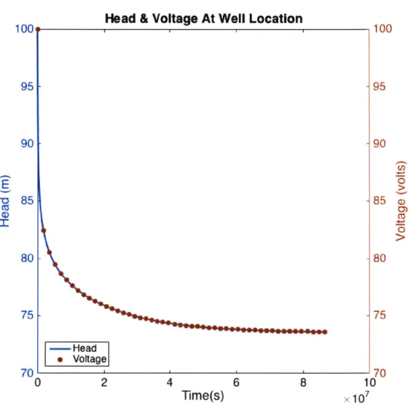
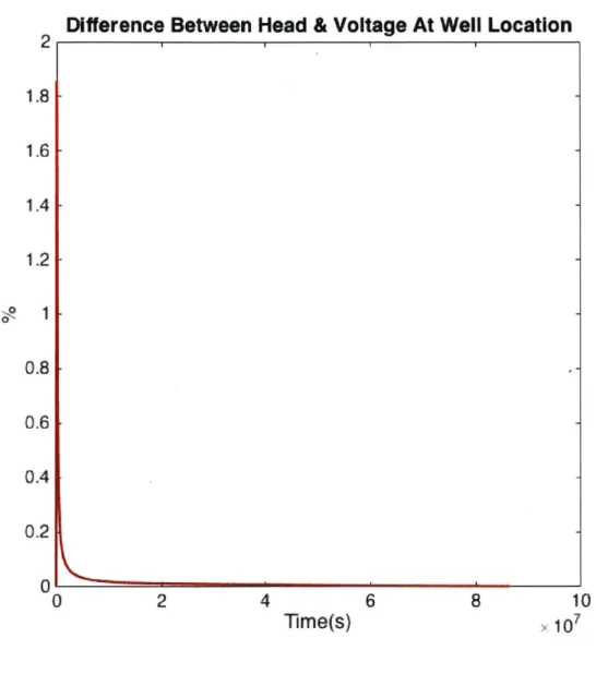
. Now, the result of the hydraulic modeling will be compared with the RC circuit solution. Figure 3-7 shows a simplified RC circuit. The boundary conditions are represented by voltage sources at all ends. Head and voltage at the well location are plotted in Figure 3-8 to compare the results. Figure 3-9 shows the percentage difference between voltage and head. The RC simulation fits the hydraulic model excellently. The difference does not exceed 2% between the two approaches.

VY

C

I

VI

t\/\/\

AV/VCu

A

VCI

MVA-'V v

7K

k)NN/

Figure 3-7: 3 x 3 RC circuit that has a constant voltage source on all sides and current output at the center.

100

95

Head & Voltage At Well Location

901 85 a) I

80

Time(s)

6

8

10

Figure 3-8: The solid line is the the result of the hydraulic finite difference solution. The red dots are the result of the RC simulation. Voltage was scaled to head using the scaling factors equal to 1.

2

0

0

Difference Between Head & Voltage At Well Location

2

4

Time(s)

6 8 10

10 7

Figure 3-9: The percent difference between the RC and hydraulic approaches.

45

The second example consists of different boundary conditions: the Dirichlet type boundary still describes two boundaries of the aquifer while the other two conditions

are no flow boundaries, (Figure 3-10). The aquifer is homogeneous with a single

hydraulic conductivity similar to the one in the previous example. At t > 0, the aquifer is pumped out at a constant flow rate. Figure 3-11 displays the results of the finite difference solution.

Constant (h) 00 hi=100 No flow X 3 1000m

Figure 3-10: Schematic of the aquifer. The dimension of the aquifer is 1. 000m x

1, 000m. The initial hi is 100m. Dirichlet boundaries are represented by specific h

equal to 100m at east and north boundaries. Q is the constant discharge rate. The

rest of the boundaries are no flow.

Again, results from the hydraulic simulation were compared with those of the electric RC circuit solution. The RC circuit is similar to figure 3-7 except that high resistance values represent the south and west boundaries. Figure 3-12 shows the

comparison between the two approaches. The percent difference between the two

solutions is plotted in Figure 3-13. This example shows that the two approaches are in good agreement.

* ww. x - - ______ - -- * m

Hydraulic Conductivity Map (n/day)

200 400 3 80I9 XIml 1000 b) 1. L 0. Cb

1000 Head Distribution (m) after 500 days

800 -700~ 600

/

Head Across The Reservoir

10100ay 90 85 80-100 _days 51o1 days 700days 900days 70 200 400 600 800 1000 X(M)

Figure 3-11: a) Hydraulic conductivity in (x, y) coordinates. b) The head distribution in plan view after 500 days of pumping. c) Transient head response at the well location. d) Evolution of head across the aquifer marked by the dashed line on figure b.

47 Hydraulic Head at The Well

1: 90 85 80 75 70

Head & Voltage At Well Location

1001

00

Time(s)

107

Figure 3-12: The solid line is the finite difference solution of the fluid equations. The dots are the result of RC simulation.

1.4

1

Difference Between Head & Voltage At Well Location

.2 [

0

0.6

0.21-0

2

Time(s)

Figure 3-13: The percent difference between the RC and hydraulic approaches for the second example.

In the third example, a single well pumps water at a constant flow rate from an aquifer surrounded by constant head boundaries (Figure 3-14). A set of two hydraulic

conductivities, K1 and K, , are supplied in the model. Figure 3-15 presents the

sinmulation results. Figures 3-17 and 3-18 compare the results of the two simulation methods. Constont (h) 00 E

~

Figure 3-14: Schematic of the aquifer. The bottom is an impermeable boundary.

The dimension of the aquifer is 1000m x 1000,m. The initial h is 100m. Dirichlet

boundaries are represented by specific h equal to 100m at the four boundaries. Q is

the constant discharge rate.

The RC network appears to do a great job of simulating the fluid flow. It does not matter how complex the model is; the electric analog produces a response that matches the hydraulic system. However, the CPU time for simulating both systems varies clue to the different methods of solving the two equations.

Hydraulic Conductivity Man im/da)v b)

p

Head Distribution (m) after 500 days

sL

X m

C)

Hydraulic Head at The Well

d)

Head Across The Reservoir

T0 8 2 4 '3 8 TiilmE'S I 10 12 14 S10 Ei - IOU days 302 ays SUL' days, -- U d0ays' 40C days o 0 U 6o B)UD Xii

Figure 3-15: a) Hydraulic conductivity in (+r, y) coordinates. b) The head distriblitiOli in plan view after 500 days of puiping. c) Head change with time at the well location.

(1) Tine evolution of head across the aquifer marked bY dashed line on figure (B).

51 a) 0 2-X1i : ; , I)i)LI I -I I, " i" . , I

Head & Voltage At Well Location

ime(s)

10

Figure 3-16: The solid line is the groundwater finite difference solution. The (lots are the result of the RC simulation.

Difference Between Head & Voltage At Well Location

Time(s)

106

Figure 3-17: The percent difference between the RC and hydraulic solutions.

53

To make a fair comparison between the two simulation, both systems were solved by finite difference. Equation (3.22) is discretized and solved using finite difference. The CPU times needed to solve the hydraulic and electrical problems were approxi-mately the same (figure 3-18), and the difference between the two solutions is almost zero.

CPU Time

100

90

80-70

60

50

40

30

-20

10

20

for Electric and Hydraulic Simulation

* Hydraulic

* Electric

40

60

Grid Size

80

100

120

Figure 3-18: The difference in CPU time for solving the two systems (hydraulic and RC) using a finite difference method.

54

I1

E

0~

U

0

0

Chapter 4

Inversion

The main objective of inversion is to determine the hydraulic conductivity K or transmissivity T and storativity S, of the aquifer from data collected in the field,

such as head h and flow rate

Q.

field but it might be done on a scale different from that of the preferred final model. For example, head measurements are limited to few observation wells. The objective is to solve the flow equations using parameters that agree with the observed data. To achieve a plausible fit between the observed data and the modeled data, model parameters must be determined at each iteration step. Figure 4-1 illustrates the road map for the inversion. A widely used method of parameter estimation demands

manual trial and error, which is expensive. This chapter discusses the theory of an automatic inversion scheme and presents examples of several inversion models.

4.1

Theory

The model parameters m describing the system is related to the observed data d through the forward model operator G such that:

G(m) = d. (4.1)

The main objective of inversion is to determine m from the observed data d. The

55

Data

Output

collection

parameters

Data is collected

-

Model parameters

from observation

are optimized to fit

wells

the true data.

Figure 4-1: The main steps of the Inversion method.

best solution exists when there is a minimum residual between the true data and the 'model' data. A commonly used measure of the misfit is the L2 -norm of the residual, which is the difference between the true data and the 'model' data. Minimizing the

L2 - norm can be achieved by obtaining a least square solution. This inversion iteratively updates the model parameters in each step using a correction vector. The damped least squares solution (Aster et al., 2005) is achieved by computing the parameter correction vector 6m as follows:

6Tm (ATA+ -' 6~IlTd. (4.2)

where A is the Jacobian matrix, I is the identity matrix, a is the regularization

'damping' parameter, and 6d is the data difference vector. For relatively small scale

problems, Singular Value Decomposition (SVD), which is mathematically robust and numerically stable, can be used to solve Eq (4.2). oz is a scalar value that controls the speed of convergence of the solution.

The Jacobian "A" matrix is numerically calculated by the partial derivatives of the data with respect to the parameters. Then, data(n) x parameters(m) matrix A is decomposed into the product of three matrices: