HAL Id: hal-01221343
https://hal.inria.fr/hal-01221343
Submitted on 27 Oct 2015
HAL is a multi-disciplinary open access
archive for the deposit and dissemination of
sci-entific research documents, whether they are
pub-lished or not. The documents may come from
teaching and research institutions in France or
abroad, or from public or private research centers.
L’archive ouverte pluridisciplinaire HAL, est
destinée au dépôt et à la diffusion de documents
scientifiques de niveau recherche, publiés ou non,
émanant des établissements d’enseignement et de
recherche français ou étrangers, des laboratoires
publics ou privés.
Automatic evolutionary medical image segmentation
using deformable models
Andrea Valsecchi, Pablo Mesejo, Linda Marrakchi-Kacem, Stefano Cagnoni,
Sergio Damas
To cite this version:
Andrea Valsecchi, Pablo Mesejo, Linda Marrakchi-Kacem, Stefano Cagnoni, Sergio Damas. Automatic
evolutionary medical image segmentation using deformable models. 16th IEEE Congress on
Evolu-tionary Computation (CEC’14), Jul 2014, Beijing, China. pp.97-104, �10.1109/CEC.2014.6900466�.
�hal-01221343�
Automatic Evolutionary Medical Image
Segmentation using Deformable Models
Andrea Valsecchi
∗, Pablo Mesejo
†§, Linda Marrakchi-Kacem
‡, Stefano Cagnoni
†and Sergio Damas
∗∗European Centre for Soft Computing, Mieres, Spain {andrea.valsecchi, sergio.damas}@softcomputing.es †Deparment of Information Engineering, University of Parma, Italy {pmesejo, cagnoni}@ce.unipr.it ‡Neurospin, CEA, Gif-Sur-Yvette. CRICM, UPMC Universit´e Paris 6, France [email protected]
§ISIT-UMR 6284 CNRS, Universit´e d’Auvergne, Clermont-Ferrand, France
Abstract—This paper describes a hybrid level set approach to medical image segmentation. The method combines region-and edge-based information with the prior shape knowledge introduced using deformable registration. A parameter tuning mechanism, based on Genetic Algorithms, provides the ability to automatically adapt the level set to different segmentation tasks. Provided with a set of examples, the GA learns the correct weights for each image feature used in the segmentation.
The algorithm has been tested over four different medical datasets across three image modalities. Our approach has shown significantly more accurate results in comparison with six state-of-the-art segmentation methods. The contributions of both the image registration and the parameter learning steps to the overall performance of the method have also been analyzed.
I. INTRODUCTION
Image segmentation (IS) is the process of partitioning an im-age into different regions according to a specific criterion [1]. Most image analysis techniques use IS to create a meaningful representation of the content of the image and to detect, locate and measure the objects of interest.
Medical IS is a challenging task due to poor image contrast, noise, diffuse organ/tissue boundaries, and imaging artifacts. Moreover, the segmentation of complex anatomical regions often requires that one consider simultaneously a variety of factors, such as texture, absolute and relative intensity differences, shape, organs spatial location, etc. In this context, automatic IS techniques are required to detect multiple features of the image, and then to combine the information that have been gathered with some source of prior knowledge about the structure being segmented.
The development of such approaches, combining different sources of image information, has been a major goal of IS research [2], [3]. However, these techniques usually have a very application-specific design, so that a method used to segment one object can hardly be adapted to another task. There are at least two important issues in creating a more flexible, automatic segmentation framework. First, the fine tuning of the parameters involved in the definition of the segmentation criterion, which is complicated and time consuming. Second, creating a source of prior information (e.g. an active appearance model) is usually a long, complex process that requires human intervention. This second point also limits the applicability of machine learning techniques to ease the parameter tuning phase.
In [4], we introduced Hybrid Level Set (HLS), a segmen-tation framework for medical images, combining region, edge and prior shape information. The algorithm uses a machine learning process, based on a Genetic Algorithm (GA), to automatically adapt the segmentation method to different kinds of images and target regions. Significantly, the learning process only requires some segmentation examples, rather than application-specific knowledge, therefore it can be easily applied to any kind of segmentation problem.
The original study compared HLS with a number of estab-lished segmentation algorithms on several different segmenta-tion datasets, finding that the new evolusegmenta-tionary segmentasegmenta-tion algorithm delivered a statistically significant improvement over all competitors. However, although the overall performance of the method was excellent, we did not investigate extensively the benefit of the learning process over the segmentation results. The main contribution of this work is to extend the research performed in [4] by studying the contribution of the tuning to the final results. To this end, we replicated the original experimental study using different approaches for the machine learning step, comparing our GA with random and grid search, two popular techniques in parameter tuning. The new results are integrated in the previous experimentation, creating a more comprehensive comparison and justifying the use of GA.
This paper is structured as follows: in section II we provide the theoretical foundations necessary to understand our work. In section III, a general overview of the method is presented, providing details about the evolutionary tuning procedure of the different terms in the deformable model. Finally, section IV presents the statistical analysis of the results, followed, in section V, by some final remarks and a discussion about possible future developments.
II. BACKGROUND
Before describing HLS, we briefly review two main con-cepts involved in its design: level sets and image registration. A. Level sets
The term “deformable models” (DMs) [5] refers to curves or surfaces, defined within the image domain, that move under the influence of “internal” forces, related with the curve features, and “external” forces, related with the features of the image
regions surrounding the curve. Internal forces enforce regular-ity constraints and keep the model smooth during deformation, while external forces are defined to attract the model toward features of the object of interest.
Starting from an initial location and shape, a DM is iter-atively modified by applying various shrink/expansion oper-ations according to some energy function or force. A DM can be represented either by a set of parameters, such as the locations of a sequence of points, or using a geometric/implicit representation. Active Contour Models (ACM) [6] and Active Shape Models (ASM) [7] belong to the former approach, while the Level Set (LS) method [8] is an example of the latter.
In LS, the region being segmented, denoted Γ, is represented as the zero level set of a n + 1-dimensional function φ, i.e. Γ(t) = {x | φ(t, x) = 0}. The dynamics of φ can be described by the following general form:
∂φ
∂t + F |∇φ| = 0
known as the LS equation, where F is called the speed function and ∇ is the spatial gradient operator. F defines the segmentation criterion to be followed, since it can depend on position, time, the geometry of the interface (e.g., its normal or its mean curvature), or different image features.
B. Image Registration
Image registration (IR) refers to the process of geometrically aligning multiple images having some shared content [9]. The alignment is represented by a spatial transformation that overlaps the common part of the images. One image, the scene, is transformed to match the geometry of the other image, called the model. IR is formulated as an optimization problem in which the similarity between the scene and the model after the transformation is maximized. The optimization is usually performed using classic gradient-based numerical optimization algorithms [10], [11] or approaches based on evolutionary algorithms and other metaheuristics (MHs) [12], [13].
In this study, image registration is used as a preliminary step in a segmentation process. We assume to have an atlas available (i.e., a typical or average image of the anatomical region to be segmented), in which the target region has been already labeled. The atlas-based segmentation process [14] begins by registering the atlas to the input image. Then, the region of the target image that overlaps the labeled region in the atlas is the result of the segmentation process.
C. Related works
In a large number of contributions, evolutionary techniques or other MHs have been used to evolve DMs. Indeed, segmen-tation can be formulated as an optimization problem in which the target function to minimize is the combination of internal and external forces. This target function can be very complex (noisy, highly-multimodal) and the classic algorithms often fail to minimize it [15]. Hence, the global search capabilities of MHs can be very beneficial. For instance, in [16] and [17], ACMs are combined with an optimization procedure based on GAs. In [18] a GA evolves a population of medial-based
shapes extracted from a training set, using prior shape knowl-edge to produce feasible deformations while also controlling the scale and localization of these deformations. Also, MHs can be used for parameter tuning [19] or in the preliminary processing of the input images [20]
III. HLSMETHOD
A. Level set and force definition
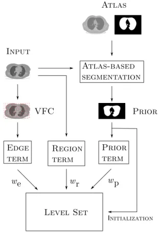
HLS combines edge, region and prior shape knowledge of the target object to guide the LS evolution [4]. Figure 1 provides an overview of HLS. The LS is characterized by its initial position and the force that guides its evolution. In what follows, we will detail these two components.
Atlas-based
segmentation
Atlas
Prior
Input
Level Set
VFC
Prior
term
Region
term
Edge
term
Initializationwe
wr
wp
Figure 1: The schematic view of the interaction among the components of HLS.
In its first stage, using an atlas of the target object, HLS performs atlas-based segmentation of the image under con-sideration. This requires the availability of a single image of a similar target object, along with its segmentation. The initial registration-based step provides a prior segmentation that will allow the LS to start its evolution near the area to be segmented. This benefits both the speed and the accuracy of the segmentation since, with a default initialization over the whole image, features located far from the target area are more likely to negatively influence the evolution of the LS. The registration process, based on the algorithm proposed in [21], has two stages. It begins with affine registration, which removes large misalignments between the images. Then, a
deformable B-Spline-based registration takes care of adjusting the overlap locally and match the finer details.
After initialization, the LS moves under the influence of three force terms called region, edge and prior terms. The total force acting on the LS is a linear combination of the force terms
Ftot= wrFr(C) + weFe(C) + wpFp(C, P ) (1)
where C is the current contour and P is the prior segmentation. Along with the specific parameters of each term, the use of weights provides flexibility to our approach, allowing it to be adapted to the features and particularities of the objects to be segmented.
The region term (Fr) minimizes the inhomogeneity of the
intensity values inside and outside the surface enclosed by the evolving contour. It is borrowed from the classic “Active Contours Without Edges” (CV) [22] method by Chan and Vese. The idea is to separate the image into two regions having homogeneous intensity values. More formally, the process minimizes the energy functional shown in Equation 2.
Fr(x, y, C) =
(
λ1 |I(x, y) − IC|2 (x, y) ∈ C
λ2 |I(x, y) − IΩ\C|2 (x, y) 6∈ C
(2) The edge term (Fe) attracts the curve towards natural
boundaries and other edges of the image. It is based on Vector Field Convolution (VFC) [23]. First, an edge map of the target image is obtained applying Gaussian smoothing followed by the Sobel edge detector [24]. Then, the edge map is convolved with a vector field kernel K in which each vector points to the origin. The magnitude of the vectors decreases with the distance d, in such a way that distant edges produce a lower force than close edges (the actual value is 1/dγ+1). For a point c of contour C, the edge term is simply the normal component of the VFC with respect to C.
Finally, the prior term (Fp) moves the LS towards the prior
segmentation P obtained by the registration. Note that this is rather different than just using the prior as initial contour for the LS, as the prior term can balance the other forces when they are small or inconsistent, leading to a more “conservative” segmentation. To compute the prior term, we calculate the region term on the prior image, rather than on the target image. This way the prior force moves the LS towards the prior segmentation and its module is proportional to the overlap between the current contour and the prior.
B. Parameter learning
A defining feature of HLS is the ability to learn opti-mal parameter settings for every specific dataset. Provided a training set of already segmented images of the same class, the parameters are learned using a classic machine learning approach: configurations of parameters are tested on the training data, and the results are compared with the ground truth to assess their quality.
In the original study, the parameter tuning was performed by a GA. GAs have been extensively applied to the tuning of
image segmentation methods [17], [18], as well as in a large number of other areas. In this extended study, we consider two additional classic techniques for comparison purposes. These are grid search and random search, which are the most widely used techniques in parameter tuning [25] thanks to their efficiency and simple design.
For our segmentation algorithm, the parameter learning step aims to adjust the weights of the force terms wr, we, wp and
their corresponding parameters λ1, λ2 (region term) and γ
(edge term). The quality of a configuration s is the average quality of the segmentations obtained using the parameters values in s. In this case, we measured the average Dice coef-ficient (DSC) obtained segmenting the images in the training set. DSC measures set agreement: a value of 0 indicates no overlap with the ground truth, and a value of 1 indicates perfect agreement.
In this context, the use of grid and random search is straight-forward. The GA, instead, has been designed for solving a continuous optimization problem. Solutions are strings of real numbers encoding the values of the mentioned parameters. The population is created at random, drawing the parameters’ values in their corresponding ranges with uniform probability. The remaining components are tournament selection, blend crossover (BLX-α) [26], random mutation [27] and elitism.
Notice that some segmentation steps do not depend on all parameters. For instance, the VFC of an image depends only on γ, therefore the computation of the VFC can be shared among different configurations having the same value of γ. This led to a very large speedup in the learning process, especially for the creation the prior, which is the most com-putationally demanding step in the segmentation process by far.
IV. EXPERIMENTALSETUP
The aim of the experimental study is to assess the per-formance of our proposal with a particular emphasis on its ability to adapt to different medical segmentation tasks. To this end, we use four datasets representing different anatomical structures across three image modalities. After introducing the datasets and a selection of comparison methods, we present the results of the experiments and their analysis.
A. Datasets
Three kinds of biomedical image modalities were used to verify the global performance of the different methods over different datasets. We focused our interest on microscopy histological images derived using In Situ Hybridization, X-Ray computed tomography, and magnetic resonance imaging.
• In Situ Hybridization-derived images (ISH). 26 mi-croscopy histological images were downloaded from the Allen Brain Atlas (ABA) [28]. The anatomical structure to segment was the hippocampus.
• Magnetic Resonance Imaging (MRI). A set of 17 T1
-weighted brain MRI were retrieved from a NMR database with their associated manual segmentations [29]. The
deep brain structures to segment were caudate, putamen, globus pallidus, and thalamus.
• X-Ray Computed Tomography (CT). A set of 10 CT images were used in the experiments [30]. Four of them correspond to a human knee and the other six to human lungs.
All four datasets, considering lungs and knee as different image sets, were randomly divided in training and test data. The training images were used by HLS for the learning of the parameters, while the test images were the ones used in the final experiments to check the segmentation performance of the methods. In ISH, 22 images were used for testing and 4 as a training set. As atlas for the registration, the actual references in the ABA were employed to obtain the shape prior. With respect to MRI, 3 images were used as training set, another 3 were used as atlas, and the remaining 11 as test set. Finally, in relation to CT, one image of every organ was used as training and atlas for the registration, leaving 3 lung and 2 knee images for testing the system.
B. Segmentation methods included in the comparison In our comparisons we have included both deterministic and non-deterministic methods, as well as classic and very recent proposals. The stress has been focused on DMs, and their hybridization with MHs, but other kinds of approaches have also been taken into account.
• Soft Thresholding (ST) [31]. This deterministic method, presented in 2010, is based on relating each pixel in the image to the different regions via a membership function, rather than through hard decisions, and such a mem-bership function is derived from the image histogram. Having been successfully applied to CT, MRI and ultra-sound, it seemed interesting to apply it also to microscopy histological images and compare its performance with other state-of-the-art methods.
• Atlas-based deformable segmentation (DS) [21]. This
method refers to the atlas-based segmentation procedure used in HLS to compute the prior (see section III). This is actually a stand-alone segmentation method, therefore it is included in the experimental study as a representative of registration-based segmentation algorithms. Moreover, comparing DS’s and HLS’s results will assess the influ-ence of the prior term on the performance of the second method. During the whole study, the setup and the atlas selection mechanism of DS are always the same whether the method is used stand-alone or embedded in another segmentation technique.
• Geodesic Active Contours (GAC) [32]. This technique, introduced in 1997, connects ACM’s based on energy minimization and geometric active contours based on the theory of curve evolution. In this paper, two implemen-tations of GAC have been tested. The first one uses as initial contour the whole image, while the second one, called DSGAC, employs the segmentation obtained using DS to create the initial contour of the geometric DM.
• Chan&Vese Level Set Model (CV) [22]. This implicit DM was also included in the comparison to check its performance in comparison with the other approaches. Also in this case, like in GAC, two implementations have been tested. The first one uses the whole image as initial contour, and the second one employs the segmentation result obtained by DS as the LS initial contour.
C. Parameter settings
As HLS has an automatic parameter learning phase, it would be unfair to compare it against other methods without some kind of parameter tuning. In general, we want the competitors to deliver their best performance, regardless of their parameter sensitivity or their ability to be tuned. Therefore, we decided to tune the competitors with an extensive search using the test data, rather than the training one. This means the results reported for all methods but HLS are actually the best average results they can obtain on these datasets. This gives them a clear advantage over HLS, as for the latter the parameters are learned using the training data only.
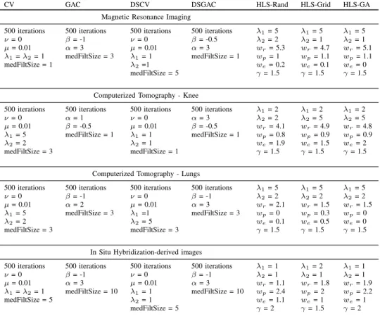
For CV, GAC, DSGAC and DSCV, all the possible com-binations of the values in Table I were tested. Moreover, for DSGAC and DSCV, 10 different initial masks were created using DS and the best one was used in the tuning. The number of iterations for GAC and CV was set to 500 to ensure the process reached convergence. With respect to the parameters used in ST and DS, all configurations were taken from the original proposals [4].
For HLS, we ran each of the three parameter learning approaches over the training data, obtaining three different configurations. Then, we tested HLS on the test data, leading to three sets of results, denoted GA, Grid and HLS-Rand according to the algorithm used for the tuning. We matched the amount of resources of each tuner, in this case the number of parameter configurations to be tested, as well as the search space. For the GA, the size of the population was set to 50 individuals, and the evolution lasted 50 generations. The probability of crossover and mutation was set to 0.7 and 0.1, respectively, and the size of the tournament was 3. The range of λ1, λ2was restricted to {1, 2, 5} to match the settings
used with the other methods.
The final parameters configurations are reported in Table II. It is interesting to remark how the tuning detected a different level of importance for each term across the datasets. For instance, if we consider HLS-GA, in MRI the edge term is not used (we= 0) since our machine learning system determines
that, for a good segmentation, the region term and prior shape knowledge are enough. When segmenting CT images of the lungs the only term used is the region-based one. In this case, λ1 and λ2 were set to 5 and 2, respectively. This means that
our final segmentation will have a more uniform foreground region (since the energy contributed by the “variance” in the foreground region has a larger weight), at the expense of allowing more variation in the background.
Table II: Parameters obtained after tuning ST, GAC, CV, DSGAC, DSCV, and training HLS.
CV GAC DSCV DSGAC HLS-Rand HLS-Grid HLS-GA Magnetic Resonance Imaging
500 iterations 500 iterations 500 iterations 500 iterations λ1= 5 λ1= 5 λ1= 5 ν = 0 β = -1 ν = 0 β = -0.5 λ2= 2 λ2= 1 λ2= 1 µ = 0.01 α = 3 µ = 0.01 α = 3 wr= 5.3 wr= 4.7 wr= 5.1 λ1= λ2= 1 medFiltSize = 3 λ1= 1 medFiltSize = 1 wp= 1 wp= 1.1 wp= 1.1 medFiltSize = 1 λ2=1 we= 0.2 we= 0.1 we= 0
medFiltSize = 5 γ = 1.5 γ = 1.5 γ = 1.5
Computerized Tomography - Knee
500 iterations 500 iterations 500 iterations 500 iterations λ1= 2 λ1= 2 λ1= 2 ν = 0 α = 1 ν = 0 α = 3 λ2= 2 λ2= 5 λ2= 5 µ = 0.01 β = -0.5 µ = 0.01 β = -0.5 wr= 4.1 wr= 4.9 wr= 4.8 λ1= 5 medFiltSize = 1 λ1= 1 medFiltSize = 1 wp= 0.8 wp= 0.9 wp= 0.9 λ2= 2 λ2= 1 we= 1.9 we= 1.5 we= 2 medFiltSize = 3 medFiltSize = 1 γ = 1.5 γ = 1.5 γ = 1.5
Computerized Tomography - Lungs
500 iterations 500 iterations 500 iterations 500 iterations λ1= 5 λ1= 5 λ1= 5 ν = 0 β = -1 ν = 0 β = -1 λ2= 2 λ2= 2 λ2= 2 µ = 0.01 α = 2 µ = 0.01 α = 3 wr= 2.1 wr= 1.5 wr= 1.5 λ1= 5 medFiltSize = 3 λ1=1 medFiltSize = 3 wp= 0 wp= 0.3 wp= 0
λ2= 2 λ2= 5 we= 0.1 we= 0.5 we= 0
medFiltSize = 3 medFiltSize = 3 γ = 1.5 γ = 1.5 γ = 1.5
In Situ Hybridization-derived images
500 iterations 500 iterations 500 iterations 500 iterations λ1= 1 λ1= 2 λ1= 1 ν = 0 β = -1 ν = 0 β = -1 λ2= 1 λ2= 1 λ2= 1 µ = 0.01 α = 3 µ = 0.01 α = 3 wr= 1.1 wr= 1.8 wr= 1.9 λ1= λ2= 1 medFiltSize = 10 λ1= 1 medFiltSize = 10 wp= 2.4 wp= 2 wp= 2.2 medFiltSize = 5 λ2= 1 we= 1.1 we= 1 we= 1
medFiltSize = 5 γ = 2 γ = 1.5 γ = 2
Table I: Combination of parameters tested for CV, GAC, DSCV and DSGAC. Parameter Values α contour weight {1, 2, 3} β expansion weight {-1, -0.5} µ weightLengthTerm {0.01, 0.1, 0.25, 0.5, 0.75} λ1 { 1, 2, 5} λ2 { 1, 2, 5} size median filter {1, 3, 5, 10} minimum size allowed {1, 50, 75, 100, 200, 5000, 25000}
D. Experimental results
DS, DSCV, DSGAC and HLS are non-deterministic al-gorithms, since stochastic methods, like Scatter Search, are embedded in them. To estimate their performance we ran 20 repetitions per image and computed mean, median and standard deviation values over the whole set of results (see Table IV). For instance, in ISH the mean DSC value of DS is 0.876, and represents the average of 440 experiments performed (20 repetitions per image over 22 images).
We also performed a statistical analysis of the results. When comparing two methods, we used Wilcoxon rank-sum test [33], a non-parametric test that checks whether one of two samples tends to have larger values than the other. Unlike t-test, Wilcoxon’s does not require the samples to be normally distributed. As multiple comparisons were performed, Holm’s correction [34] was applied to the p-values.
In Table III, some concise information about the running time of each algorithm is provided with an illustrative purpose.
The fastest method is ST with MRI, taking only 1 second per image, while the slowest are the different applications of HLS to ISH, employing up to 10 minutes to process an image. Nevertheless, several factors affect the accuracy of a comparison in terms of execution time. Some of the methods have been developed in MATLAB and others in C++. Also, the nature of the algorithms is completely different, making them hardly comparable.
Table III: Average execution time per method and kind of image. All values are in seconds; they were obtained running the experiments on an Intel Core i5-2410M @ 2.3GHz with 4.00 GB of RAM. The programming environment has also been reported.
Language ISH Knee Lungs MRI ST MATLAB 39 2.5 1.7 1 CV MATLAB 87 67 36 11 GAC MATLAB, C++ 32 16 15 1.5 DSCV MATLAB, C++ 582 310 384 429 DSGAC MATLAB, C++ 493 265 342 407 DS C++ 471 245 326 404 HLS C++ 545 252 331 405
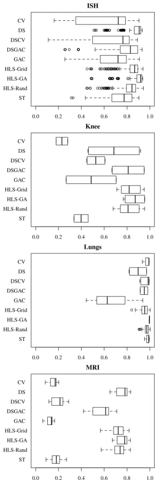
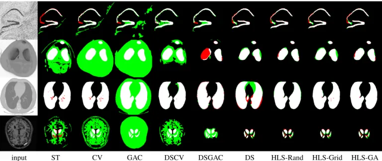
The experimental results are reported in Table IV. Visual examples of segmentations obtained by the methods on each dataset are provided in Figure 3.
The performance of the segmentation methods varies greatly across the four datasets. The easiest problem to be solved has been the segmentation of Lungs in CT images, with all methods but GAC scoring higher than 0.85. The most complex
task has shown to be the segmentation of deep anatomical structures in brain MRI, where four of the compared methods have obtained an average DSC of 0.2 or less.
The per-dataset results are shown in Figure 2 using boxplots and in Table V through the average rankings. Obviously, the performance of every method depends on the nature of the image to be segmented. For instance, techniques based on grey intensity level (such as CV and ST) yielded worse results in image modalities with less contrast and small differences in terms of pixel intensity like MRI.
HLS-GA has obtained the best results in all biomedical image datasets. It achieved the best values for the mean DSC and it was ranked as the best method in every image modality. The Wilcoxon test (Table V) showed, with very high confidence, that the difference between HLS-GA and the other methods is statistically significant in all but one case (DS on MRI). This behavior is also robust, as shown by the low standard deviation values. We can then conclude that HLS-GA is the best segmentation method in the comparison.
Despite providing a good overall performance, both HLS-Grid and HLS-Rand obtained inferior results compared to HLS-GA in all datasets. We can then conclude that the GA has provided a significantly more effective strategy for the parameter learning. This could be explained by the trade-off obtained by the GA between search space exploration and exploitation of promising solutions. Note that with a different learning approach, HLS would not have delivered such a clearly superior performance with respect to the competitors. The DS method has been one of the best-performing algo-rithms, ranking at the top over three datasets. More in general, all methods using the registration-based initialization scored better than those using a standard one. This applies also to CV and GAC: in all but one case, both DSCV and DSGAC ranked better than their counterpart, with a statistically significant difference.
Overall, DSGAC delivered an acceptable performance, ranking above average in three datasets out of four. This is remarkable, as the regular GAC ranked constantly in the last three positions, and it can be explained by the high sensitivity of GAC to its initialization.
DSCV ranked around average in all datasets, performing slightly worse, although more consistently, than DSGAC. The plain CV method achieved a bad performance, ranking last or second to last in three datasets. Only on the Lungs dataset, where the grey value is enough to segment the target quite accurately, CV delivered good results.
ST results showed a similar pattern to CV. It performed better than CV, but being ST based on the histogram it showed limited ability to cope with complex scenarios. On the other hand, ST is the fastest method on the group and it has virtually no parameters to be set.
V. DISCUSSION ANDFUTURERESEARCH
Through an extensive experimentation, we proved that HLS is an accurate and flexible segmentation method. It ob-tained excellent results with all the medical image modalities
0.0 0.2 0.4 0.6 0.8 1.0 ST HLS-Rand HLS-GA HLS-Grid GAC DSGAC DSCV DS CV ISH 0.0 0.2 0.4 0.6 0.8 1.0 ST HLS-Rand HLS-GA HLS-Grid GAC DSGAC DSCV DS CV Knee 0.0 0.2 0.4 0.6 0.8 1.0 ST HLS-Rand HLS-GA HLS-Grid GAC DSGAC DSCV DS CV Lungs 0.0 0.2 0.4 0.6 0.8 1.0 ST HLS-Rand HLS-GA HLS-Grid GAC DSGAC DSCV DS CV MRI
input ST CV GAC DSCV DSGAC DS HLS-Rand HLS-Grid HLS-GA Figure 3: Some visual examples of the results obtained. One image per image modality has been selected: the first row corresponds to ISH, the next one to CT-Knee, and the last two to CT-Lungs and MRI. White represents true positives (correctly segmented areas), red false negatives (areas that should have been segmented but they were not), and green false positives (areas that were segmented but they should have not been segmented).
Table IV: Segmentation Results using Dice Similarity Coeffi-cient (DSC). Values are sorted in descending order.
Dataset Method Dice Coefficient mean median stdev
ISH HLS-GA 0.888 0.918 0.079 DS 0.876 0.907 0.078 HLS-Grid 0.845 0.867 0.081 HLS-Rand 0.823 0.843 0.084 DSGAC 0.791 0.830 0.143 ST 0.728 0.775 0.175 DSCV 0.673 0.764 0.203 GAC 0.670 0.722 0.181 CV 0.589 0.723 0.257 Knee HLS-GA 0.868 0.872 0.087 HLS-Grid 0.833 0.819 0.087 HLS-Rand 0.819 0.810 0.089 DSGAC 0.810 0.811 0.142 DS 0.687 0.685 0.227 DSCV 0.528 0.527 0.079 GAC 0.486 0.486 0.310 ST 0.398 0.398 0.088 CV 0.230 0.230 0.072 Lungs HLS-GA 0.996 0.997 0.001 ST 0.979 0.990 0.023 CV 0.973 0.992 0.034 HLS-Rand 0.970 0.973 0.023 DSCV 0.966 0.985 0.034 HLS-Grid 0.951 0.955 0.036 DSGAC 0.950 0.952 0.027 DS 0.896 0.897 0.062 GAC 0.670 0.627 0.251 MRI HLS-GA 0.758 0.780 0.048 DS 0.752 0.783 0.056 HLS-Rand 0.729 0.739 0.052 HLS-Grid 0.724 0.723 0.053 DSGAC 0.585 0.613 0.087 DSCV 0.204 0.213 0.054 ST 0.175 0.181 0.053 CV 0.155 0.171 0.042 GAC 0.124 0.139 0.035
Table V: Average rank achieved by every method per image modality and adjusted p-value of Wilcoxon test comparing each algorithm against HLS.
Dataset Method Mean Rank p-value
ISH HLS-GA 1.50 DS 2.23 0.000 HLS-Grid 3.55 0.000 DSGAC 4.50 0.000 HLS-Rand 5.14 0.000 ST 6.32 0.000 GAC 7.09 0.000 DSCV 7.14 0.000 CV 7.55 0.000 Knee HLS-GA 1.50 HLS-Grid 2.50 0.001 DSGAC 3.00 0.001 HLS-Rand 4.00 0.001 DS 4.50 0.000 DSCV 6.50 0.000 GAC 7.00 -ST 7.50 -CV 8.50 0.000 Lungs HLS-GA 1.00 ST 2.67 -CV 3.67 0.000 DSCV 4.33 0.000 HLS-Rand 4.67 0.000 DSGAC 6.33 0.000 HLS-Grid 6.33 0.000 DS 7.00 0.000 GAC 9.00 -MRI HLS-GA 1.27 0.000 DS 1.91 0.460 HLS-Rand 3.27 0.000 HLS-Grid 3.73 0.000 DSGAC 4.82 0.000 DSCV 6.18 0.000 ST 7.09 0.000 CV 7.73 0.000 GAC 9.00 0.000
under consideration, outperforming well-consolidated tech-niques. Thanks to the tuning procedure developed, it performs an automatic self-adaptation of its parameters depending on the anatomical structure and image modality at hand.
We have also proven the key role played by the Genetic Al-gorithm, as other popular tuning strategies did not provide such excellent results. In particular, the outcome of the comparison would have been different without the GA, with HLS ranking mostly above average instead of taking the top position in all datasets.
The main drawback of HLS is that it is not as fast as ST. This is obvious since it can be as fast as its components and, evidently, DS is a deformable registration process that can take several minutes on a general-purpose computer. More sophis-ticated implementations, like GPGPU programming, can be tested to speed-up the computations. Finally, the introduction of a textural term could be taken into consideration if the benefits obtained with its use justify it.
ACKNOWLEDGMENTS
This work has been supported by Ministerio de Economia y Competitividad under project SOCOVIFI2 (TIN2012-38525-C02-01 and TIN2012-38525-C02-02), including EDRF fund-ing. NMR database is the property of “CEA/I2BM/NeuroSpin” and can be provided on demand to [email protected]. Data were acquired with PTK pulse sequences, reconstructed with PTK reconstructor package and postprocessed with Brain-visa/Connectomist software.at http://brainvisa.info.
REFERENCES
[1] D. L. Pham, C. Xu, and J. L. Prince, “Current Methods in Medical Image Segmentation,” Annual Review of Biomedical Engineering, vol. 2, pp. 315–337, 2000.
[2] J. Malik, S. Belongie, T. Leung, and J. Shi, “Contour and texture analysis for image segmentation,” International Journal of Computer Vision, vol. 43, no. 1, pp. 7–27, Jun. 2001.
[3] Y. Zhang, B. J. Matuszewski, L.-K. Shark, and C. J. Moore, “Medical Image Segmentation Using New Hybrid Level-Set Method,” in Procs. of the International Conference BioMedical Visualization: Information Visualization in Medical and Biomedical Informatics, 2008, pp. 71–76. [4] P. Mesejo, A. Valsecchi, L. Marrakchi-Kacem, S. Cagnoni, and S. Damas, “Biomedical image segmentation using geometric deformable models and metaheuristics,” Computerized Medical Imaging and Graphics, 2014, article in press. [Online]. Available: http://www. sciencedirect.com/science/article/pii/S0895611113002024
[5] D. Terzopoulos and K. Fleischer, “Deformable models,” The Visual Computer, vol. 4, pp. 306–331, 1988.
[6] M. Kass, A. Witkin, and D. Terzopoulos, “Snakes: Active contour models,” International Journal of Computer Vision, vol. 1, pp. 321–331, 1988.
[7] T. F. Cootes, C. J. Taylor, D. H. Cooper, and J. Graham, “Active shape models-their training and application,” Computer Vision and Image Understanding, vol. 61, pp. 38–59, 1995.
[8] J. Sethian, Level Set Methods and Fast Marching Methods: Evolving Interfaces in Computational Geometry, Fluid Mechanics, Computer Vision, and Materials Science, ser. Cambridge Monographs on Applied and Computational Mathematics. Cambridge University Press, 1999. [9] B. Zitov´a and J. Flusser, “Image registration methods: a survey,” Image
and Vision Computing, vol. 21, pp. 977–1000, 2003.
[10] F. Maes, D. Vandermeulen, and P. Suetens, “Comparative evaluation of multiresolution optimization strategies for image registration by maximization of mutual information,” Medical Image Analysis, vol. 3, no. 4, pp. 373–386, 1999.
[11] S. Klein, M. Staring, and J. P. W. Pluim, “Evaluation of optimization methods for nonrigid medical image registration using mutual informa-tion and b-splines,” IEEE Trans. on Image Processing, vol. 16, no. 12, pp. 2879–2890, 2007.
[12] S. Damas, O. Cord´on, and J. Santamar´ıa, “Medical image registration using evolutionary computation: An experimental survey,” IEEE Com-putational Intelligence Magazine, vol. 6, no. 4, pp. 26 –42, nov. 2011. [13] A. Valsecchi, S. Damas, and J. Santamar´ıa, “Evolutionary
intensity-based medical image registration: a review,” Current Medical Imaging Reviews, vol. 9, no. 4, pp. 283–297, 2013.
[14] M. Cabezas, A. Oliver, X. Llad´o, J. Freixenet, and M. B. Cuadra, “A review of atlas-based segmentation for magnetic resonance brain images,” Computer Methods and Programs in Biomedicine, vol. 104, no. 3, pp. e158 – e177, 2011.
[15] P. Mesejo, R. Ugolotti, F. D. Cunto, M. Giacobini, and S. Cagnoni, “Automatic hippocampus localization in histological images using differ-ential evolution-based deformable models,” Pattern Recognition Letters, vol. 34, no. 3, pp. 299 – 307, 2013.
[16] L. Ballerini, “Genetic snakes for medical images segmentation,” in Evo-lutionary Image Analysis, Signal Processing and Telecommunications, 1999, vol. 1596, pp. 59–73.
[17] D.-H. Chen and Y.-N. Sun, “A self-learning segmentation frame-work—the taguchi approach,” Computerized Medical Imaging and Graphics, vol. 24, no. 5, pp. 283 – 296, 2000.
[18] C. McIntosh and G. Hamarneh, “Medial-based deformable models in non-convex shape-spaces for medical image segmentation using genetic algorithms,” IEEE Trans. on Medical Imaging, vol. 31, no. 1, pp. 33–50, 2012.
[19] M. Heydarian, M. Noseworthy, M. Kamath, C. Boylan, and W. Poehlman, “Optimizing the level set algorithm for detecting object edges in mr and ct images,” IEEE Trans. on Nuclear Science, vol. 56, no. 1, pp. 156 –166, 2009.
[20] C.-Y. Hsu, C.-Y. Liu, and C.-M. Chen, “Automatic segmentation of liver pet images,” Computerized Medical Imaging and Graphics, vol. 32, no. 7, pp. 601 – 610, 2008.
[21] A. Valsecchi, S. Damas, J. Santamar´ıa, and L. Marrakchi-Kacem, “Intensity-based image registration using scatter search,” Artificial In-telligence in Medicine, vol. 60, no. 3, pp. 151–163, March 2014. [22] T. F. Chan and L. A. Vese, “Active contours without edges,” IEEE Trans.
on Image Processing, vol. 10, pp. 266–277, Feb. 2001.
[23] B. Li, S. Member, S. T. Acton, and S. Member, “Active contour external force using vector field convolution for image segmentation,” IEEE Trans. on Image Processing, vol. 16, pp. 2096–2106, 2007.
[24] R. C. Gonzalez and R. E. Woods, Digital Image Processing, 2nd ed. Addison-Wesley, 2001.
[25] J. Bergstra and Y. Bengio, “Random search for hyper-parameter optimization,” J. Mach. Learn. Res., vol. 13, pp. 281–305, Feb. 2012. [Online]. Available: http://dl.acm.org/citation.cfm?id=2188385.2188395 [26] L. J. Eshelman and J. D. Schaffer, “Real-coded genetic algorithms and interval-schemata.” in Foundation of Genetic Algorithms 2, D. L. Whitley, Ed. San Mateo, CA: Morgan Kaufmann., 1993, pp. 187–202. [27] T. B¨ack, D. B. Fogel, and Z. Michalewicz, Handbook of Evolutionary Computation. IOP Publishing Ltd and Oxford University Press, 1997. [28] Allen Institute for Brain Science, “Allen Reference Atlases,” http:
//mouse.brain-map.org, 2004-2006.
[29] C. Poupon, F. Poupon, L. Allirol, and J.-F. Mangin, “A database dedicated to anatomo-functional study of human brain connectivity,” in Proceedings of the 12th Annual Meeting of the Organization for Human Brain Mapping, no. 646, Florence, Italy, 2006.
[30] N. Bova, ´O. Ib´a˜nez, and O. Cord´on, “Image segmentation using extended topological active nets optimized by scatter search,” IEEE Computa-tional Intelligence Magazine, vol. 8, no. 1, pp. 16–32, 2013.
[31] S. Aja-Fernandez, G. Vegas-Sanchez-Ferrero, and M. Martin Fernandez, “Soft thresholding for medical image segmentation,” in Proc. Interna-tional Conference of the IEEE Engineering in Medicine and Biology Society (EMBC), 2010, pp. 4752 –4755.
[32] V. Caselles, R. Kimmel, and G. Sapiro, “Geodesic active contours,” International Journal of Computer Vision, vol. 22, pp. 61–79, 1997. [33] W. H. Kruskal, “Historical notes on the wilcoxon unpaired two-sample
test,” Journal of the American Statistical Association, vol. 52, no. 279, pp. 356–360, 1957.
[34] S. Holm, “A simple sequentially rejective multiple test procedure,” Scandinavian Journal of Statistics, vol. 6, no. 2, pp. 65–70, 1979.