CaPETITIVE ADVANTAGE AND COLLUSION by
Richard Schnalensee
Competitive Advantage and Collusion
Richard Schmalensee
Alfred P. Sloan School of Management Massachusetts Institute of Technology
ABSTRACT
In oligopoly models, the symmetric case is special theoretically and neglects asymmetries that may be important empirically. This essay analyzes the implications of cost differences for collusive oligopoly equilibria. Four different technologies for effecting collusion, which are essentially identical in the symmetric case, are considered. Axiomatic bargaining models are employed with simple functional forms to produce quantitative measures of the effects of cost differences and numbers of rivals. Low-cost firms with large shares in Cournot equilibrium are seen to have little to gain from collusion. Implications for the estimation and interpretation of conjectural variations are explored.
1. Introduction_ _ _ _ _ _ _ _ _ _ _
The main objective of this study is to begin to fill a gap in the literature on oligopoly theory by systematically exploring the implications of long-lived efficiency differences for collusive equilibria. Once beyond
existence theorems, most treatments of oligopoly theory focus on the symmetric case.1 But Demsetz (1973), Porter (1985) and others have stressed the
empirical importance of long-lived differences in efficiency, broadly defined, and it has become standard, following Iwata (1974), to allow for such differ-ences in econometric studies of particular industries.2 The symmetric
case is thus of doubtful empirical relevance. And, as I hope this essay makes clear, the symmetric case turns out to be very special theoretically. When firms' costs differ, so do the implications of a variety of techniques for effecting collusion that are essentially equivalent in the symmetric case. The simplest possible model, which is easily analyzed when costs are equal, becomes an algebraic mess when they are not.
A number of recent works on oligopoly theory that allow for cost differ-ences assume, generally without much discussion, that the objective of
collusion is the maximization of total industry profits.3 But, as Bain (1948) argued persuasively almost 40 years ago in an incisive comment on Patinkin's (1947) classic paper, this objective makes sense only when side payments are possible.4 When side payments are not possible, colluding sellers face a relatively complicated bargaining problem that has not been systematically analyzed. In general, total industry profits may have to be reduced in order to attain an equitable division of gains from collusion; there may be an equity/efficiency tradeoff. A second objective of this
II1
study is to apply the tools of cooperative bargaining theory to explore the range of likely--solutions to this problem.5
Most empirically-oriented discussions of oligopolies with cost differ-ences stress the fact that collusion is more complex than in the symmetric case because firms' preferred prices differ.- (ee, for instance, Blair and Kaserman (1985, pp. 145-6) or Scherer (1980, pp. 156-60).) And casual empiricism suggests that effective collusion is indeed relatively rare- in the presence of substantial competitive advantage. (IBM has been accused of many things! collusion is not one of them.) But complexity may not be the only reason for this. If a leading firm's cost advantage over its rivals is great enough, non-cooperative behavior yields it approximately its monopoly profits. That is, the maximum possible gains to a low-cost leader from collusion go to zero as its cost advantage increases. Since collusion involves costs and (both legal and other) risks, one would not expect to observe it when the low-cost firm has little to gain. In the limit as the leader's cost advantage increases, then, the probability that collusion will be attempted goes to zero.
This limiting argument is of little empirical interest, however. The more interesting question involves the likely gains to a low-cost firm from collusion when cost differences are moderate, so that the aggregate share of high-cost firms in non-collusive equilibrium is not negligible. The third objective of this study is to examine the magnitude of the low-cost firm's potential gains in such situations, in order to evaluate the likely empirical importance of the limiting argument advanced aove. This objective requires numerical evaluation of alternative equilibria. This approach is also made
attractive by the algebraic complexity of the simple model employed here when costs differ.
The remainder of this essay is organized as follows. Section 2 sets out the assumptions and notation employed. Section 3 describes and compares
four alternative collusion technologies, three of which are equivalent in the special symmetric case. The conjectural variations representation of collusive equilibria is also discussed. Section 4 describes the solution
concegts employed- to characterize collusive outcomes and compares some of their general implications. Section 5 presents the results of applying
those concepts to each of the four technologies described in Section 3. The main results of this study and their implications are briefly summarized in Section 6.
2.AssumRtions and Notation
I consider a market for a homogeneous product in which one low-cost firm faces competition from N identical high-cost sellers. This permits me to vary the intensity of non-cooperative rivalry in a tractable fashion. In most of the analysis, the market demand function is taken to be linear.
With appropriate choice of units for money and output, the inverse demand function can thus be written as
P * P(Q) - 1 - gI (1)
where P is market price and Q is total output.
The low-cost firm, which will be referred to as the leader or firm 1 in what follows, is assumed to have costs given by
li
where q is the leader's output and 81 is a constant between zero and one. The assumption of constant unit costs and neglect of capacity constraints is consistent with a focus on long-lived differences in costs or products. Let
nl
be the leader's profit.The high-cost firms, which will be referred to as followers or firms of type 2, also have constant unit costs:
C(q2) = (1 - 82)q2, (3)
where q2 is the output of a single follower, and 82 is a constant between zero and one. The two cost parameters must satisfy 82 < E < 282. (The second of these inequalities ensures that the followers' costs are below the leader's monopoly price, 81/2.) Let Nn2 be total followers' profit.
These functional form assumptions produce a model that is algebraically simple, at least as compared to other asymmetric oligopoly models. This
model also has the convenient property, which basically derives from relations involving similar triangles, that as long as attention is limited to relative (i.e., percentage) changes in such quantities as profit and consumers'
surplus, only the ratio R 81/82 matters. The market is thus effectively described by two parameters, R and N. On the other hand, the use of specific functional forms necessarily limits the generality of the results.
I assume that if collusion does not occur, the market is in Cournot equilibrium. The Cournot point serves in what follows as a benchmark for
evaluating the effects of collusion as well as the status quo point in collusive negotiations. The Cournot assumption has a number of advantages. First, it is familiar and tractable. Second, it has the realistic implica-tion, not shared by the natural Bertrand alternative, that high-cost sellers have positive market shares. Third, following Kreps and cheinkman (1983),
it assigns central importance to capacity decisions and is thus consistent with the long-ruif focus of this inquiry. Note that under this assumption the leader/follower distinction refers only to market shares; there is no behavioral asymmetry.
The ratio R is difficult to relate to observables, as it reflects both cost differences and the potential profitability of the market considered. To see this, let R' (1-82)/(1-81), the ratio of followers' to leader's
unit cost. A bit of algebra then yields
R 81/ - R'(1-81)3. (4)
Increases in R' clearly increase R. But, since R' exceeds one, R is a decreasing function of 81. For any given value of R', R is thus lower the
more profitable the market would be to firm as a monopolist. Accordingly, R can best be thought of as measuring the importance of the leader's cost advantage relative to potential market profitability. But, for the sake of brevity, I will refer to R simply as the leader's cost advantage in what follows.
To provide a closer link to observables, we can describe the market by N and S, where S is the share of the leader in Cournot equilibrium. The relation among these parameters is easily shown to be the following:
R N(I+S)/(N+1-S). (5)
Increasing S or N, with the other parameter held constant, increases the leader's cost advantage. The larger is N, the more intense is competition, and the larger the leader's cost advantage must be to sustain any given market share. Note also that the condition 1 < R < 2 corresponds to 1/(N+1) < S < 1.
The alternative to Cournot equilibrium is assumed to be perfect collus-ion, in the sense that a point on the relevant profit-possibility frontier is chosen.6 I turn first to a discussion of alternative frontiers and then consider alternative rules for selecting the collusive point.
3. _Cllusion Technologies and Coniectural Variations
Depending on the methods available for affecting collusion, the litera-ture suggests four alternative profit-possible frontiers. Since the followers have identical and constant costs, each follower's share of total follower profit is just equal to its share of total follower output. We thus lose no generality by dealing throughout with average follower output and profit, q2 and n2, respectively.
Side Payments (SP) If the colluding firms can make side payments (or merge), all production will be done by the leader. Total collusive output will thus equal the leader's monopoly output, 1/2, and total profit will equal the leader's monopoly profit, ( )2/4. (Note that this neglects any short-run fixed costs associated with followers' capacity.) This simplest technology is represented by the straight line labeled SP in Figure 1 and by the similarly-labeled point in Figure 2. In both Figures, the point labeled C corresponds to the Cournot equilibrium. (Figures 1 and 2 are approximate representations of the case N 2 and R 1.143 (or S .455), a case with relatively unimportant cost differences.) It is perhaps best to think of the SP technology as a standard of comparison, rather than as a realistic possibility in many situations.
Market Sharing_ MS) If side payments are ruled out for legal or other reasons, each firm's earnings derive only from its own production and sales.
(In Bain's (1948) phrase, "earnings follow output.") Profit possibilities are thus restricted as compared to the side payments technology, since production must be inefficient if both types of firms receive positive profits, The market sharing technology is most commonly assumed in such
situations: firms are assumed to set and abide by output quotas. It is demonstrated in the Appendix that for constant marginal costs and !ny demand
function satisfying the second-order conditions, the profit-possibilities frontier is strictly convex, as is the curve labeled MS in Figure 1. Rising marginal cost is necessary but not sufficient for total industry profit to attain a local maximum at a point where ql and q2 are both positive.
When demand and cost are given by equations (1) - (3) above, it is straightforward to use the first-order conditions for maximization of n2
subject to a lower bound on in to solve for profits of the two types of firms as functions of total output along the collusive frontier:
l = [(81-Q) 2(2Q-82)]/(81-82) (6a)
Nn2 = (82-2) (8 -2Q)3/(81-82). (6b)
From these equations it is easy to show that as one moves to the northwest along the MS locus in Figure 1, total industry output falls from the leader's monopoly output, 81/2, to the followers' monopoly output, 82/2, and total profit falls accordingly.
The same first-order conditions yield an explicit expression for the contract curve labeled MS in Figure 21
II1
This curve is strictly convex, as drawn. (Bishop (1960, p. 948) asserts the convexity of the contract curve in this case.) The leader's market share declines as one moves to the northwest along this curve.
Market Division (MD) When the relevant frontier in a bargaining problem is non-concave, one normally thinks of using mixed strategies to convexify the feasible set. This seems unnatural here, however. If a coin were to be flipped once to decide which type of firm were permitted to monopolize the market, some enforcement mechanism would be required to compel the loser(s) to exit. Even if such a mechanism could be imagined, one would have to allow for risk-aversion in evaluating the expected payoffs from alternative coins and. Alternatively, if a coin were to be flipped many times, so that average profits per period equaled expected profits in the limit, firms would have to start up and shut down frequently. Neither scenario resembles any obvious example of actual cartel behavior.
But an alternative convexification device does correspond to a frequently-observed pattern of cartel behavior, the firms can divide the market.7 That is, each actual or potential customer can be assigned to a single firm. If all customers are identical, as I will assume for simplicity, and firm one is allocated a fraction W of them, its inverse demand curve is given by PP(q1/W), and it will charge its monopoly price. Firms of type 2 will similarly charge their higher monopoly price to the customers they have been allocated. tarting from any point on the MS contract curve, if each
firm is given a share of customers equal to its market share at that point, all will be able to increase profits by changing price.
Because market division requires different prices for the same product when sellers' costs differ, it is clearly feasible only when some mechanism can be used to rule out arbitrage at moderate cost. When such a mechanism
is available, the profit-possibility frontier (gross of the costs of
preventing arbitrage) becomes the locus labeled MD in Figure 1. The corres-ponding contract curve is similarly labeled in Figure 2. Note that production is inefficient under market division, as under market sharing. Profit
possibilities are lower under the latter technology because firms with different costs sharing the same market impose what amounts to a negative
externality on each other. This occurs because, except at the extreme points, all must depart from their preferred price.
When costs are equal, the SP, MS, and MD loci coincide in both Figure 1 and Figure 2. In this symmetric case, and only in this case, the division of monopoly output among colluding sellers does not affect total industry profit.
PEoRErtional Reduction (PR) In many situations in which side payments are impossible, arbitrage will prevent market division. Moreover, the complexity of the market sharing technology when costs differ may make long and complex negotiations necessary, especially when firms are imperfectly informed about their rivals' costs, and this may entail unacceptable antitrust risks. In such situations, colluding sellers may resort to simple rules to set output quotas.
One such rule that immediately suggests itself involves maintaining market shares at their non-collusive (Cournot) values and reducing the output of all sellers proportionately. This constrains the firms to move along the PR line in Figure 2. By doing so they can reach a point on the MS contract curve and enjoy the corresponding profits.B In the symmetric case, this point maximizes total industry profit and divides it equally among all sellers. When costs differ, however, this point has no special attraction.
Movements in toward the origin along the PR curve in Figure 2 produce movements away rom the Cournot point, C, on the PR locus in Figure 1. The tangency of this latter locus and the M contract curve always occurs above the Cournot point; it occurs to the left of that point, so that the leader is worse off than in Cournot equilibrium, if (1+S) > 1 and the following condition is satisfiedl
N > (1-S2)/(82 + S - 1). (8)
The right-hand side of this expression is a decreasing function of S. For N=I, the leader is worse off at the intersection of the PR and MS loci than at the Cournot point if S>.781. As N increases, the critical value of S declines, approaching .618 in the limit. Firms with large cost advantages will thus refuse to enter into collusive arrangements that use the propor-tional reduction technology to reach the market sharing contract curve. Alternatively, if the market sharing technology is employed, such firms will require a higher market share than at the Cournot equilibrium; a point on the MS locus to the right of its intersection with the PR locus will
accordingly be chosen.
ConjIctural Variations When firms of both types are operating and sharing the market, as in Cournot equilibrium or in collusive equilibria produced by the MS or PR technology, one can describe behavior either by the sellers' outputs or by the corresponding implied conjectural derivatives. The conjectural derivative of any firm i is defined, as usual, as X. = t(dQ/dqi) - 13. This is to be understood as the increase in its rivals' total output that firm i expects to occur as a response to a small unit increase in its own output. Then, corresponding to any vector of seller
outputs, there exists a vector of Xi such that the first-order conditions for individual profit-maximization are satisfied.
Particularly in collusive equilibria, it makes little sense to think of observed behavior as actually involving this sort of maximization. But, following the pioneering work of Iwata (1974), a number of authors have
estimated conjectural derivatives econometrically. This approach can best be understood as providing a convenient summary description of market behavior, which may in fact involve a complex mix of cooperative and non-cooperative elements. The Appendix explores the implications of MS and PR collusion for implied X1 in a general asymmetric odel. It is shown there that if one
leader faces N identical followers, then under any cost and demand conditions satisfying the relevant second-order conditions, MS collusion implies
N + (N-1)X1 -XIX 2 = . (9)
This expression is positive under PR collusion at points outside the MS contract curve in Figure 2. It is negative at points inside that curve.
4. Collusive Solution Concepts
All reasonable solution concepts impose individual rationality. That is, they limit attention to outcomes at which all parties are at least as well off as at the status quo point. This serves to limit attention to points to the northeast of C in Figure 1, between the two dashed lines. The solution concepts discussed below satisfy this requirement for all values of N and R. (This discussion relies on Roth's (1979) excellent development of axiomatic bargaining theory.) In the descriptions that follow I use an asterisk to denote a collusive outcome and a super-script c" to denote the
III
Cournot status quo point. As above, attention is confined to collusive equilibria in wich the (identical) followers are treated identically.
Nash In the classic Nash (1950) solution, the product of the parties' gains,
(H* c)(H* c)N n 1 2 n2 is maximized along the relevant frontier.
Kalai-Smorodinsky (K-S) To compute the solution proposed by Kalai and Smorodinsky (1975), define nm as the maximum profit the leader can receive on the relevant frontier when all followers receive their status quo profit, and define n as the maximum profit a single follower can receive when the leader and the other N-1 followers receive their status quo profit. The K-S solution is then the point on the frontier satisfying
(n'-
c)/(Hm
T-
c) (f*
-
Rc)/(f
-
f2).
(10)If the profit-possibility frontier is linear, as implied by the SP and MD technologies, it is easy to show (using the ability to allocate total follower profit arbitrarily among followers) that the Nash and K-S solutions coincide. Under the PR technology all followers must have the same profit, so that n2
is given by the intersection of the vertical dashed line and the PR locus in Figure 1.
EgualGains(E6) Roth (1979, pp. 92-97) suggests the possible relevance of solutions in which the absolute gains to all parties are equal:
(n - 3 n ). (11)
Along the SP frontier, it is easy to show that the Nash, K-S, and EG solutions all coincide. Thus all firms gain an equal absolute dollar amount from
collusion in all three general bargaining solutions. (In relative terms, of course, the followers gain more than the leader because their status quo profits are lower.)
Along the flatter MD frontier in Figure 1, the E solution lies to the left of the Nash/K-S solution. The latter thus gives the low-cost firm a greater absolute gain than each high-cost firm. If the PR technology is employed, no solution satisfying (12) exists when N 1. And when N 2, the EG solution maximizes firm 's profit on the PR frontier.
IWAS In the MD technology, a natural focal point (in the sense of
Schelling (1960)) is provided by the allocation of customers to firms in the original Cournot equilibrium. Accordingly, for this technology only, I consider solutions in which W*, the fraction of customers assigned to the leader, equals S, the leader's initial market share. Each follower than receives a fraction (1-S)/N of the market demand curve. This is the only obvious focal point solution that satisfies individual rationality for all N and S.9
5._Collusive Eguilibria
Under the SP and MD technologies, the equilibria corresponding to the Nash/K-S, E, and (MD only) W*=S solutions can be obtained explicitly as
functions of N and S. Under the PR technology, the K-S and EG equilibria can be also obtained analytically. All the formulae involved are too complex
to be informative, however. Moreover, under the MS and PR technologies, numerical solution of equations is necessary to obtain values for Nash equilibria, and the K-S and E equilibria must also be treated numerically under the MS technology. Accordingly, this Section adopts a purely numerical
II1
approach. Alternative equilibria are presented for some illustrative parameter values, and general relations revealed by computation of many equilibria are discussed. 10
Two implications of cost differences should be kept in mind in inter-preting the results that follow. First, when costs differ, production in the original Cournot equilibrium is inefficient. The possibility of rationalizing production gives rise to potential gains from collusion that are not present in the symmetric case. Second, when costs differ, the
low-cost firm's profit in Cournot equilibrium exceeds that of its rivals. As I noted in Section 1, this limits the leader's potential gains from collusion.
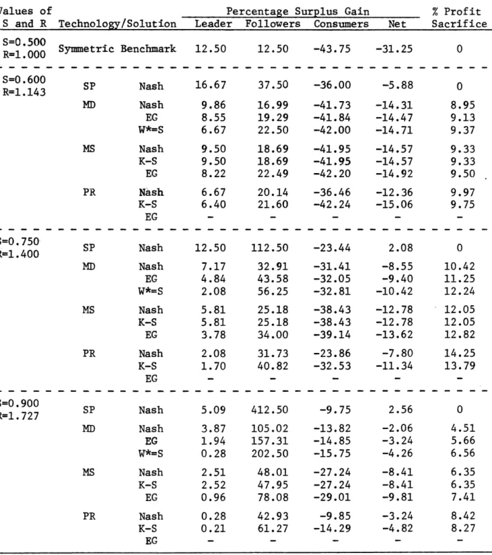
Consider Table 1, which describes the effects of alternative forms of collusion in the duopoly case. When costs are equal, the natural symmetric collusive equilibrium raises both firms' profits by 12.5%, lowers consumers' (Marshallian) surplus by 43.75%, and produces a reduction in total surplus of 31.25%.T1 In all the asymmetric equilibria in Table 1, as in all I have examined, the leader's percentage gain from collusion is below the followers', and the difference rises with increases in the leader's Cournot share. This of course reflects in part the difference in their initial, noncollusive profits.
When the leader's cost advantage is small (Ra1.143), all parties do better in relative terms under SP collusion than in the symmetric case
because production is rationalized. As the leader's cost advantage increases, its percentage gain decreases, the follower's percentage gain increases, and consumers' percentage losses decrease. It is straightforward to show that SP collusion produces a net gain in (Marshallian) social welfare if
The critical value of S (R) falls from .692 (1.294) to .200 (1.200) as N increases. All collusive equilibria computed under the other three tech-nologies involve a net social loss.
If the SP technology is not employed, total industry profits are not maximized. The last column in Table 1 gives the percentage by which total
industry profits fall short of their maximum value. For all values of N and all non-SP equilibria, this profit sacrifice is maximized for moderate
values of R. As R approaches one, the sacrifice goes to zero as the symmetric case is approached, while as R approaches two, the followers' significance approaches zero.
All parties are generally substantially worse off in collusive equil-ibrium if the SP technology is not employed. For any given technology not involving side payments, outcomes more favorable to the leader are also more favorable to consumers, since the leader prefers a lower price than the followers.
The differences between the MD and MS solutions are relatively small, as are those between the MS/Nash and MS/K-S equilibria. These patterns reflect the near-linearity of the MS profit-possibility frontier for most
values of N and S. (This was noted by Bishop (1960, p. 948).) The PR solution is surprisingly close to the other two in some cases, though it is generally clearly inferior from the leader's viewpoint. Because it precludes rationalizing production by increasing the leader's share, the extent to which total output can be restricted is limited, and consumers are often better off under PR collusion than if the MD or MS technologies had been employed.
III
In the examples of MD collusion described in Table 1, the W*=S solution lies to the left of the Nash and EG solutions along the MD frontier. This implies that the Nash and ES solutions involve W*>S, so that the leader's share of customers (and, a fortiori, of output) is increased by collusion. For large N and small R, however, the W*=S solution can be more favorable to the leader than either of the others. When this occurs, Nash or E collusion involves a reduction in the leader's share of customers. In extreme cases, the leader's share of output may be lower than at the Cournot point.
Efficiency calls for an increase in the leader's share, but potential ration-alization gains are small when R is near one, and equity considerations
become important when N is large.
Under the MS technology, when the Nash and K-S solutions differ
noticeably, as they do for large values of R or N, the latter is more favor-able to the leader. Both are to the right of the E solution along the MS frontier. The leader's collusive market share exceeds S at all MS equilibria in Table 1. But, as under the MD technology, collusion may involve reducing the leader's market share when R is small and N is large. Also as above, this occurs most often in the E solution.
Along the PR locus, the Nash solution generally involves a smaller output reduction than the K-S solution and is thus better for the leader. When N 2, the E solution is better for the leader than either of the others. For N > 2, it is worse than the others except for R very close to two.
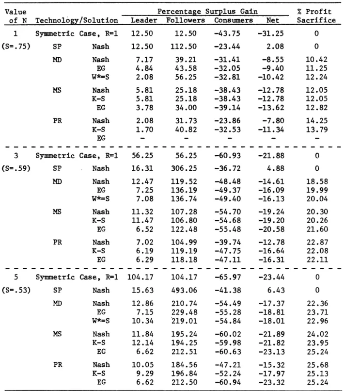
Table 2 shows the effect of changes in N, with R held constant at a moderate level. In the symmetric case, increases in N simply increase the intensity of competition at the status quo point and thus increase the
however, increases in N also increase the aggregate bargaining power and status quo share of the high-cost followers. The latter effect increases the potential gains from rationalizing production. The increased bargaining power of the followers as N increases tends to increase the profit sacrifice made in the interests of equity when side payments are impossible, as the last column in Table 2 shows.
Followers' percentage gains tend to increase with N, reflecting both their increased bargaining power and the corresponding fall in their status quo profits. For small values of R and N, the leader's relative gains tend to rise with N, reflecting the increasing potential gains from rationalizing production. Otherwise, the bargaining power effect dominates, and increases in N reduce the leader's relative (and, a fortiori, absolute) gains. (The borderline values of N and R depend on the technology and solution concept, as Table 2 reveals.)
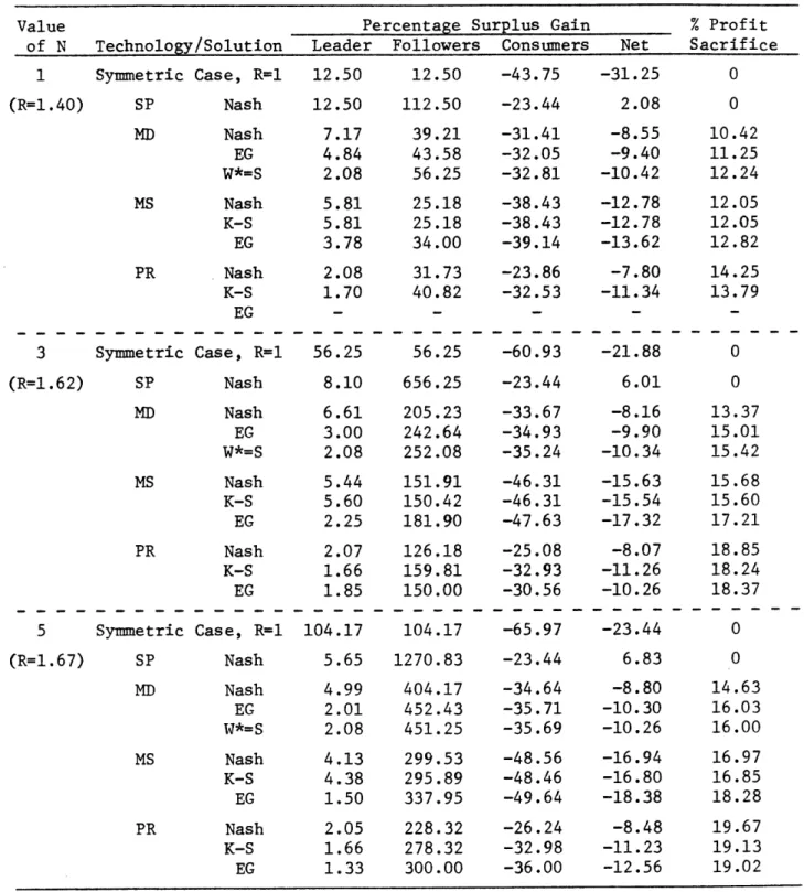
Table 3 shows the effect of increases in N when S is held constant, so that R rises with N. The pattern shown there thus reflects the effects of changes in both R and N discussed above. The followers' gains accordingly rise more rapidly with N than in Table 2, the leader's gains are more likely to decline, and the profit sacrifice and consumers' losses rise less rapidly with N than in Table 2.
Tables I - 3 indicate that in the presence of substantial competitive advantage, corre§ponding to large R the leader's gains from collusion are likely to be small, both relative to status quo profits and to gains in the symmetric case. This is particularly clear if side payments and market division are ruled out. While the leader's potential relative gains do not approach zero rapidly as R increases, they seem small relative to likely year-to-year fluctuations for values of R and N that might be encountered in
i
practice: see especially Table 3. (Note also that the figures shown deal only with economic profits; the corresponding percentage increases in the accounting profits reported to shareholders are likely to be much smaller.) It thus seems likely that the absence of gains commensurate with the risks involved tends to make collusion less likely than otherwise in the presence of substantial competitive advantage.12
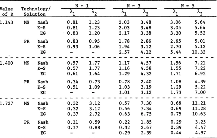
Finally, Table 4 presents the conjectural derivatives consistent with a variety of MS and PR collusive equilibria. In all equilibria examined, the leader's conjectural derivative, Xi, is less than the followers', X2. As
Table 4 indicates, the difference between these parameters can be quite dramatic. If estimates of this sort were obtained econometrically in some market, there would be a tendancy to characterize the followers as more
concerned about competitive reactions than the leader. But, by construction, the parameter values in Table 4 characterize solutions to cooperative games, not differences in expectations or competitive behavior.
When either the MS or the PR technology is employed, both parameters tend to increase with N, as condition (9) suggests. Holding N constant, increases in R tend to lower X1 and to raise X2 in MS collusion. Under the PR technology, increases in R tend to lower both parameters, but several exceptions to this rule are visible in Table 3. As cost differences are increased, it becomes harder to make large proportional reductions in output without making the leader worse off. Consistent with this, all of the PR equilibria shown in Table 4 correspond to points outside the MS contract curve (where, in the notation of the Appendix, > 1), except for the three ES equilibria in the upper right-hand corner of the Table.
6, Conclusion!
Symmetric oligopoly models may lack empirical relevance; they are certainly very special theoretically. Even with functional forms selected for tractability, relaxation of the assumption of symmetry gives rise to considerable albegraic complexity. Four technologies for affecting collusion that are essentially equivalent in the symmetric case are quite distinct when sellers' costs differ. Numerical analysis of collusive solutions
implied by axiomatic bargaining theory reveals a variety of distinctions and effects not present in the symmetric case.
Two of these seem particularly important for applied work. First, if a leading firm's cost advantage is substantial, its likely gains from collusion are relatively small. Accordingly, collusion is unlikely to be observed in the presence of substantial competitive advantage. Second, conjectural derivatives consistent with perfect collusion may vary substantially from
firm to firm, depending on the nature of collusion, the importance of cost differences, and the number of sellers. Differences in estimated conjectural derivatives may thus reflect bargaining outcomes, not differences in rivalrous behavior.
II1
APPENDIX
This Appendix explores two aspects of the market sharing technology under general cost and demand conditions. First, we examine conditions for convexity of the profit-possibilities frontier. Second, we describe points on that frontier in terms of conditions on conjectural derivatives. The latter conditions are relevant to the use of estimated conjectural derivatives to describe seller behavior, following Iwata (1974).
For the case of two firms or two groups of identical firms, the profit-possibilities frontier is obtained by maximizing 112 subject to the constraint
n
- k 0, for k between zero and firm 's monopoly profit. The constraint will be binding in this range, and the corresponding multiplier, , will thus be positive. By the envelope theorem, at an optimum will equal-d22*/dk = -dn2/dnl, where n2* is the constrained maximum of n2. The profit-possibilities frontier, 2 = n2*(nl) ' will thus be convex if and only if d+/dk is negative.
Totally differentiating the first-order conditions for a constrained maximum of 2 and the constraint with respect to k and solving by Cramer's rule, one obtains
d+/dk = - [(1-p) )2 + X(2P'+A) + X2(2+P'+A) - XI1X2]/D, (A1)
where A P(fq1+q2), Xi = d2Ci/dqi2 for i 1,2, and D is the determinant of the bordered Hessian. The second-order conditions for constrained maximization require D to be positive. In the constant cost case, X=X2=O, and strict convexity follows immediately for any demand function satisfying the second-order conditions. By continuity, the collusive frontier will also be strictly convex for any demand function if marginal costs are rising slowly enough. In order for the profit-possibilities frontier to be concave
at any point, so that total profits attain a local or global maximum with both firms (or types of firms) producing, marginal costs must be rising sufficiently rapidly.
Let us now consider description of points along this frontier in terms of conjectural derivatives. Let there be T firms, all of which may have different cost functions, and let q-i be the output of all firms except firm
i. Then firm i's conjectural derivative, Xi, is its expectation of dqi/dqi. Re-arranging the first-order condition for maximization of firm i's profits,
it is easy to see that the conjectural derivative consistent with equilibrium at any qi, q-i pair is given by
= -(P - C + qiP')/qi P ', (A2)
where C is firm i's marginal cost.
Points on the MS collusive frontier correspond to points at which n is maximized subject to the constraints ni - ki > 0, i = 2,...,T. These
constraints will all be binding in the relevant region. Let i > 0 be the multiplier corresponding to the constraint on firm i's profits. Writing out the first-order conditions for this problem and substituting from (A2), we
obtain the equations that describe a point on the MS profit-possibilities frontier in terms of the conjectural derivatives:
-X 1 ' I z1
1 -X 1 z
2 2
· . 0, (A3)
1 i or' -Xi
II1
Since the zi are all positive, it follows from (A3) that all conjectural derivatives are positive at a collusive equilibrium.1 3 Setting the
determinant of the matrix on the left of (A3) equal to zero, one obtains the necessary and sufficient condition for perfect collusion, the Iwatacondition:
T
t E X i = 1, (A4)
il
where i = /(l+Xi) for all i. Equation (A4) is equivalent to Iwata's
(1974, p. 961) equation (6.12).
Since is a continuous function of the vector of outputs and (assuming that Xi > -1 for all i) is zero only on the market sharing contract curve in output space, it must have the same sign for all points above this curve. Consider a set of small output changes, qi, i=l,...,T. The corresponding changes in profits are given by
ani = (P-ci)(.i - q i). , (A5)
where i = qi /&Q for all i. Since the i sum to unity, a necessary and sufficient condition for there to exist a set of output increases (decreases) that raise the profits of all sellers is clearly t < 1 ( > 1). Thus
exceeds unity at all points above the MS contract curve in output space. The quantity 1/9 accordingly provides a natural measure of the extent to which industry behavior is collusive. This quantity is generally confined to the unit interval, though < 1 is implied by use of the PR technology to reach a point strictly inside the MS contract curve in output space. (This corresponds to a point to the left of the tangency between the MS and PR
on PR outside the MS locus in Figure 2.) The numerical results in Section 5 in the text suggest that such equilibria are unlikely, however.
A few special cases of condition (A4) are worth presenting. For T 2, the condition is simply X1X2 = , and when T=3, (A4) implies
XIX2X3 - (XI+X2+X3) = 2. (A6)
When X2=X3=...= T one obtains equation (9) in the text. (The expression shown there has the sign of -1.) Finally, setting X1=X2 in that equation yields the condition for the symmetric case: Xi = (T-1) for all i. Except in this case, perfect collusion is consistent with substantial differences in implied (or estimated) Xi across firms. (See Table 4 for some examples.) When = 1, such differences should be interpreted as reflecting bargaining outcomes, not differences in rivalrous behavior.
II1
REFERENCES
Bain, J.S. "Output Quotas in Imperfect Cartels." QuarterlyJournalof Economics, Vol. 62 (August 1948), pp. 617-622.
Bishop, R.L. "Duopolys Collusion or Warfare?" American Economic Reiew, Vol. 50 (December 1960), pp. 933-961.
Blair, R. and Kaserman, D.L. Antitrust Economics, Homewood, ILi Irwin, 1985. Chandler, A.D. TheVisibleHand, Cambridgei Harvard University Press, 1977. Clarke, R. and Davies, S.W. "Market Structure and Price-Cost
Margins." Economica, Vol. 49 (August 19B2), pp. 277-287.
Demsetz, H. "Industry Stucture, Market Rivalry, and Public Policy." Journal of Law and Economics, Vol. 16 (April 1973), pp. 1-10.
Fellner, W. CmgetitionAmong the _ew, New York, Knopf, 1949.
Friedman, J. Oligoorly_Theory, Cambridge: Cambridge University Press, 1983. Fudenberg, D. and Tirole, J. "Sequential Bargaining with Incomplete
Information." Review of Economic Studies, Vol. 50 (April 1983), pp. 221-247.
Iwata, G. "Measurement of Conjectural Variations in Oligopoly." Econometrica,
Vol. 42 (September 1974), pp. 947-966.
Kalai, E. and Smorodinsky, M. "Other Solutions to Nash's Bargaining Problem." Econometrica, Vol. 43 (May 1975), pp. 513-518.
Kreps, D.M. and Scheinkman, J.A. "Quantity Precommitment and Bertrand
Competition Yield Cournot Outcomes." Bell Journal of Economics, Vol. 14 (Autumn 1983), pp. 326-337.
Nash, J.F. "The Bargaining Problem." Econometrica, Vol. 28 (April 1950), pp. 513-518.
. "Two-Person Cooperative Games." Econometrica, Vol. 31 (January 1953), pp. 128-140.
Orr, D. and MacAvoy, P.W. "Price Strategies to Promote Cartel Stability." Economica, Vol. 32 (May 1965), pp. 186-197.
Osborne, D.K. "Cartel Problems." A!mrican Economic Review, Vol. 66 (December 1976), pp. 835-844.
Osborne, M.J. and Pitchik, C. "Profit-Sharing in a Collusive
Oligopoly." Eurpgean Economic Review, Vol. 22 (June 1983), pp. 59-74. Patinkin, D. Multi-Plant Firms, Cartels, and Imperfect
Competition." Quarterly_ Journalof Economics, Vol. 61 (February 1947), pp. 173-205.
Porter, M.E. Cetitive Advantag!, New Yorkt Free Press, 1985.
Porter, R.H. "Optimal Cartel Trigger Price Strategies." Journal-of-Economic Theory, Vol. 29 (April 1983), pp. 313-338.
Roth, A.E. Axiomatic Models of Barg ainog, New York: Springer-Verlag, 1979. Scherer, F.M. Industrial Market Structure and Economic Performance, 2nd Ed.,
Chicago: Rand-McNally, 1980.
Schmalensee, R. "Do Markets Differ Much?" American Economic Review, Vol. 75 (March 1985), pp. 341-351.
Stigler, .J. "A Theory of Oligopoly." Jgurnal of Political Economy, Vol. 72 (February 1964), pp. 44-61.
III
FOOTNOTES
Much of the research reported here was performed while I was a visitor at CORE, I am indebted CIM (Belgium) for financial support, to Jacques Thisse for arranging my visit, and to him and my other hosts at Louvain for making my stay pleasant and productive. I am also grateful to participants
in seminars at CORE, LSE, and the Norwegian School of Economics and Business Administration for helpful discussions of earlier versions of this essay and to Garth Saloner for useful comments and suggestions. The usual waiver of liability applies, of course.
1. See, for instance, Friedman (1983). Osborne and Pitchik (1983) provide a recent exception to this generalization. They assume equal costs, however, and use the Nash (1953) variable-threat bargaining model to analyze the implications of differences in capacity.
2. It is perhaps also worth noting that in the FTC Line-of-Business data for 1975, industry dummy variables and market share together explain only about 20% of the sample variance of business unit profitability; see Schmalensee (1985). That is, intra-industry differences in profitability are much more important than inter-industry differences, even when the effect of market share is controlled for.
3. See, for instance, Osborne (1976) and Clarke and Davies (1982). Osborne stresses a mechanism for enforcing maximization of total industry
profit against violations of output quotas, but his mechanism rests on threats that are not fully credible (p. 839).
4. See also Fellner (1949), Bishop (1960), and, for a treatment broadly similar in spirit to that undertaken here, Osborne and Pitchik (1983). Chandler (1977, chs. 4 and 10) discusses the behavior of and problems encountered by 19th century cartels in the US.
5. I am persuaded that non-cooperative bargaining theory (see, for instance, Fudenberg and Tirole (1983)) provides a more satisfactory approach in principle. But for the purposes of the present study I need relatively simple solutions that can be applied to a static model, and
non-cooperative theory has yet to produce such solutions.
6. 1 thus ignore the possibility that a point inside the frontier will be chosen in order to enhance cartel stability. See Porter (1983) or, for an interesting precursor, Orr and acAvoy (1965). Note that the
possibility of entry is also neglected.
7. Blair and Kaserman (1985, ch. 7) discuss this device at some length. For brief discussions, see Stigler (1984) and Scherer (1980,
pp. 168-175). Market division, when possible, may serve to enhance cartel stability by facilitating detection of cheating, but our concern here is solely with its implications for profitability in the absence of cheating.
8. Even though Figure 2 suggests that the proportional reduction technology can reach a point on the MD contract curve, it should be clear that total profits at that point are less than the corresponding market division profits, since the market is in fact being shared by firms charging a single price.
II1
9. The other obvious focal point would set S*, the leader's collusive share of output, equal to S. But under MS or PR, this "solution" makes the leader worse off than at the status quo point if condition (8) in the text is satisfied Under the MD technology, the analogous condition can be shown to be S(4S+I)>1 and
N > (1+2S-3S2)/(4S2+S-1).
Any (N,S) pair satisfying condtion () in the text also satisfies this condtion, but not conversely. For N 1, the condition above is
satisfied for S > .611; as N increases, the critical declines to .390.
10. All the equilibria discussed in the text were computed for N = 1, 2,...,10, for R ranging over the interval (1.0, 2.0). Programs were written in IBM/Microsoft BASIC, Release 2.0, and executed on an IBM PC. The author will be happy to supply copies of all programs employed to anyone sending a suitable formatted diskette.
11. The general formulae for these changes in the symmetric case are as follows. Profits increase by 100xN2/[4(N+1)3X%. This quantity rises without bound as N increases (since symmetric Cournot profits go to zero as N increases). Consumers' surplus decreases by
100x[N(3N+4)]/[4(N+1)2 %. This quantity rises to 75% as N increases. Finally, total surplus falls by 100x[N(N+4)]/4(N+1)(N+3)]. The net loss due to collusion rises to 25% of the Cournot total surplus as N increases.
12. It must be recalled that stability considerations have been ignored throughout this analysis. If cost differences served in general to enhance the stability of collusive arrangements, perhaps by facilitating the choice of a price leader, this conclusion would have to be qualified to some extent.
13. The first-order conditions for an interior maximum of total industry profit are given by A3) with zi z qi for all i. From this one obtains immediately the Clarke-Davies (1982) result that i=(I-Si)/Si for all i at such a point, where Si is firm i's share of industry output.
i 4 CD J.I CD N) ZH
K
N) oI 0r 0 ED 0 o 0 r. H 00 H' (D H, CD -rl. .r. IlJ
PH 0 0 H -0 Ho rp 0 rt "0 n c 1~~ ItII'
Table 1: Collusive Equilibria, N=1
Values of Percentage Surplus Gain % Profit
S and R Technology/Solution Leader Followers Consumers Net Sacrifice
RS=.500 Symmetric Benchmark R=1.000 O-A AA SP Nash MD Nash EG W*=S MS Nash K-S EG PR Nash K-S EG SP Nash MD Nash EG W*=S MS Nash K-S EG PR Nash K-S EG S=0.750-- -- 12.50 16.67 9.86 8.55 6.67 9.50 9.50 8.22 6.67 6.40 12.50 7.17 4.84 2.08 5.81 5.81 3.78 2.08 1.70 5.09 3.87 1.94 0.28 2.51 2.52 0.96 0.28 0.21 12.50 -43.75 -31.25 37.50 16.99 19.29 22.50 18.69 18.69 22.49 20.14 21.60 112.50 32.91 43.58 56.25 25.18 25.18 34.00 31.73 40.82 412.50 105.02 157.31 202.50 48.01 47.95 78.08 42.93 61.27 -36.00 -41.73 -41.84 -42.00 -41.95 -41.95 -42.20 -36.46 -42.24 - --5.88 -14.31 -14.47 -14.71 -14.57 -14.57 -14.92 -12.36 -15.06 - --23.44 2.08 -31.41 -8.55 -32.05 -9.40 -32.81 -10.42 -38.43 -12.78 -38.43 -12.78 -39.14 -13.62 -23.86 -7.80 -32.53 -11.34 -9.75 2.56 -13.82 -2.06 -14.85 -3.24 -15.75 -4.26 -27.24 -8.41 -27.24 -8,41 -29.01 -9.81 -9.85 -3.24 -14.29 -4.82 0 0 8.95 9.13 9.37 9.33 9.33 9.50 9.97 9.75 0 10.42 11.25 12.24 12.05 12.05 12.82 14.25 13.79 0 4.51 5.66 6.56 6.35 6.35 7.41 8.42 8.27
Note: The PR/EG equilibrium does not exist when N = 1.
O-U. UUV R=1.143 S=0.750 R=1.400 S=0.900 R=1.727 SP MD MS PR Nash Nash EG W*=S Nash K-S EG Nash K-S EG
Table 2: Collusive Equilibria, R=1.40 Value of N Technology/Solution 1 Symmetric Case, R=l (S=.75) SP Nash MD Nash EG W*=S MS Nash K-S EG PR Nash K-S EG 3 Symmetric Case, R=1 (S=.59) SP Nash MD Nash EG W*=-S MS Nash K-S EG PR Nash K-S EG 5 Symmetric Case, R=l (S=.53) SP Nash MD Nash EG W*=S MS Nash K-S EG PR Nash K-S EG
Percentage Surplus Gain % Profit
Leader Followers Consumers Net Sacrifice
ii 12.50 12.50 7.17 4.84 2.08 5.81 5.81 3.78 2.08 1.70 56.25 16.31 12.47 7.25 7.08 11.32 11.47 6.52 7.02 6.19 6.29 04.17 15.63 12.86 7.15 10.34 11.84 12.14 6.62 10.05 9.29 6.62 12.50 112.50 39.21 43.58 56.25 25.18 25.18 34.00 31.73 40.82 56.25 306.25 119.52 136.19 136.74 107.28 106.80 122.48 104.99 119.19 118.18 104.17 493.06 210.74 229.48 219.01 195.24 194.25 212.51 184.56 196.84 212.50 -43.75 -23.44 -31.41 -32.05 -32.81 -38.43 -38.43 -39.14 -23.86 -32.53 -60.93 -36.72 -48.48 -49.37 -49.40 -54.70 -54.68 -55.48 -39.74 -47.75 -47.11 -65.97 -41.38 -54.49 -55.28 -54.84 -60.02 -59.98 -60.63 -47.21 -52.24 -60.94 -31.25 2.08 -8.55 -9.40 -10.42 -12.78 -12.78 -13.62 -7.80 -11.34 -21.88 4.88 -14.61 -16.09 -16.13 -19.24 -19.20 -20.58 -12.78 -16.64 -16.31 -23.44 6.43 -17.37 -18.81 -18.01 -21.89 -21.82 -23.13 -15.32 -17.97 -23.32 0 0 10.42 11.25 12.24 12.05 12.05 12.82 14.25 13.79 0 0 18.58 19.99 20.04 20.30 20.26 21.60 22.87 22.08 22.11 0 0 22.36 23.71 22.96 24.02 23.95 25.24 25.68 25.13 25.24 Note: The PR/EG equilibrium does not exist when N=l.
II1
Table 3: Collusive Equilibria, S=0.75
Value Percentage Surplus Ga
of N Technology/Solution Leader Followers Consume
Symmetric Cas SP MD Cas Cas MS PR 3 Symmetric (R=1.62) SP MD MS PR 5 Symmetric (R=1.67) SP MD MS PR ;e, R=l 12.50 Nash 12.50 Nash 7.17 EG 4.84 W*=S 2.08 Nash 5.81 K-S 5.81 EG 3.78 Nash 2.08 K-S 1.70 EG -;e, R=1 56.25 Nash 8.10 Nash 6.61 EG 3.00 W*=S 2.08 Nash 5.44 K-S 5.60 EG 2.25 Nash 2.07 K-S 1.66 EG 1.85 ;e, R=l 104.17 Nash 5.65 Nash 4.99 EG 2.01 W*=S 2.08 Nash 4.13 K-S 4.38 EG 1.50 Nash 2.05 K-S 1.66 EG 1.33 12.50 112.50 39.21 43.58 56.25 25.18 25.18 34.00 31.73 40.82 56.25 656.25 205.23 242.64 252.08 151.91 150.42 181.90 126.18 159.81 150.00 104.17 1270.83 404.17 452.43 451.25 299.53 295.89 337.95 228.32 278.32 300.00 -43.75 -23.44 -31.41 -32.05 -32.81 -38.43 -38.43 -39.14 -23.86 -32.53 -60.93 -23.44 -33.67 -34.93 -35.24 -46.31 -46.31 -47.63 -25.08 -32.93 -30.56 -65.97 -23.44 -34.64 -35.71 -35.69 -48.56 -48.46 -49.64 -26.24 -32.98 -36.00 .in % Profit Irs Net -31.25 2.08 -8.55 -9.40 -10.42 -12.78 -12.78 -13.62 -7.80 -11.34 -21.88 6.01 -8.16 -9.90 -10.34 -15.63 -15.54 -17.32 -8.07 -11.26 -10.26 -23.44 6.83 -8.80 -10.30 -10.26 -16.94 -16.80 -18.38 -8.48 -11.23 -12.56
Note: The PR/EG equilibrium does not exist when N=1. 1 (R=l.40) Sacrifice 0 0 10.42 11.25 12.24 12.05 12.05 12.82 14.25 13.79 0 0 13.37 15.01 15.42 15.68 15.60 17.21 18.85 18.24 18.37 0 14.63 16.03 16.00 16.97 16.85 18.28 19.67 19.13 19.02
-I
Table 4: Implicit Conjectural Derivatives at Collusive Equilibria
N = 1 N=3 N=5 Value Technology/ 2 of R Solution 1 2 1 2 1 2 1.143 MS Nash 0.81 1.23 2.03 3.48 3.06 5.64 K-S 0.81 1.23 2.03 3.48 3.05 5.64 EG 0.83 1.20 2.17 3.38 3.30 5.52 PR Nash 0.83 0.95 1.78 2.86 2.65 5.01 K-S 0.93 1.06 1.94 3.12 2.70 5.12 EG - - 2.57 4.12 5.44 10.32 1.400 MS Nash 0.57 1.77 1.17 4.57 1.56 7.21 K-S 0.57 1.77 1.16 4.58 1.55 7.22 EG 0.61 1.64 1.29 4.32 1.71 6.92 PR Nash 0.34 0.73 0.78 2.40 1.08 4.39 K-S 0.51 1.09 1.03 3.19 1.29 5.22 EG - - 1.01 3.12 1.73 7.00 1.727 MS Nash 0.32 3.12 0.57 7.30 0.69 11.21 K-S 0.32 3.12 0.56 7.34 0.69 11.28 EG 0.37 2.72 0.63 6.75 0.75 10.63 PR Nash 0.11 0.59 0.22 1.85 0.29 3.25 K-S 0.17 0.88 0.32 2.67 0.39 4.47 EG - - 0.29 2.39 0.44 4.97