HAL Id: hal-03080042
https://hal.archives-ouvertes.fr/hal-03080042
Submitted on 17 Dec 2020
HAL is a multi-disciplinary open access
archive for the deposit and dissemination of
sci-entific research documents, whether they are
pub-lished or not. The documents may come from
teaching and research institutions in France or
abroad, or from public or private research centers.
L’archive ouverte pluridisciplinaire HAL, est
destinée au dépôt et à la diffusion de documents
scientifiques de niveau recherche, publiés ou non,
émanant des établissements d’enseignement et de
recherche français ou étrangers, des laboratoires
publics ou privés.
biodiversity
Gregory Beaugrand, Richard Kirby, Eric Goberville
To cite this version:
Gregory Beaugrand, Richard Kirby, Eric Goberville. The mathematical influence on global
pat-terns of biodiversity.
Ecology and Evolution, Wiley Open Access, 2020, 10 (13), pp.6494-6511.
�10.1002/ece3.6385�. �hal-03080042�
6494
|
www.ecolevol.org Ecology and Evolution. 2020;10:6494–6511.1 | INTRODUCTION
One of the most fundamental curiosities in biology is to understand what influences biodiversity and its spatial and temporal distribution (Gaston, 2000; Lomolino, Riddle, & Brown, 2006). Currently, biolo-gists have described 1,233,500 species on land and 193,756 in the sea with recent estimates of the total number of species in these realms suggested to be 8,740,000 (terrestrial) and 2,210,000 (ma-rine) (Mora, Tittensor, Adl, Simpson, & Worm, 2011). Clearly, biodi-versity is not uniformly distributed between land and sea. Moreover, on land and in the sea, many taxonomic groups exhibit a latitudi-nal increase in species richness from the poles to the midlatitudes
or the equator (Gaston, 2000; Lomolino et al., 2006; Tittensor et al., 2010). What causes these latitudinal gradients in species rich-ness has been a topic of study and debate for decades (Rosenzweig & Sandlin, 1997), and more than 25 hypotheses have now been pro-posed (Gaston, 2000).
Neo-Darwinism predicts that natural selection favors the fit-test genetic composition, and we know that genetic isolation can lead to speciation to progressively fill vacant niches (Gould, 1977). However, neither natural selection nor speciation alone can explain (a) why there are more species on land than in the sea, (b) why there are different latitudinal biodiversity gradients (LBGs) exhibited on land (narrow maximum at the equator) and in the ocean (maximum Received: 17 July 2019
|
Revised: 19 February 2020|
Accepted: 19 March 2020DOI: 10.1002/ece3.6385
O R I G I N A L R E S E A R C H
The mathematical influence on global patterns of biodiversity
Gregory Beaugrand
1| Richard Kirby
2| Eric Goberville
3This is an open access article under the terms of the Creative Commons Attribution License, which permits use, distribution and reproduction in any medium, provided the original work is properly cited.
© 2020 The Authors. Ecology and Evolution published by John Wiley & Sons Ltd. 1LOG, Laboratoire d'Océanologie et de
Géosciences, CNRS, UMR 8187, Wimereux, France
2The Secchi Disk Foundation, Plymouth, UK 3Unité Biologie des Organismes et Ecosystèmes Aquatiques (BOREA), Muséum National d’Histoire Naturelle, Sorbonne Université, Université de Caen Normandie, Université des Antilles, CNRS, IRD, Paris, France
Correspondence
Gregory Beaugrand, CNRS, UMR 8187, LOG, Laboratoire d'Océanologie et de Géosciences, F 62930 Wimereux, France. Email: [email protected] Funding information
GB was funded by CNRS and EG by Sorbonne University.
Abstract
Although we understand how species evolve, we do not appreciate how this process has filled an empty world to create current patterns of biodiversity. Here, we conduct a numerical experiment to determine why biodiversity varies spatially on our planet. We show that spatial patterns of biodiversity are mathematically constrained and arise from the interaction between the species’ ecological niches and environmental variability that propagates to the community level. Our results allow us to explain key biological observations such as (a) latitudinal biodiversity gradients (LBGs) and especially why oceanic LBGs primarily peak at midlatitudes while terrestrial LBGs generally exhibit a maximum at the equator, (b) the greater biodiversity on land even though life first evolved in the sea, (c) the greater species richness at the seabed than at the sea surface, and (d) the higher neritic (i.e., species occurring in areas with a bathymetry lower than 200 m) than oceanic (i.e., species occurring in areas with a bathymetry higher than 200 m) biodiversity. Our results suggest that a mathematical constraint originating from a fundamental ecological interaction, that is, the niche– environment interaction, fixes the number of species that can establish regionally by speciation or migration.
K E Y W O R D S
observed over midlatitudes with sometimes a small diminution at the equator), (c) why the sea exhibits greater biodiversity on the seabed than in the pelagic zone, and (d) why there are more (pelagic and benthic) neritic (i.e., continental-shelf species, species occurring in areas lower than 200 m) than oceanic (i.e., species occurring in areas higher than 200 m) species.
Here, we conduct numerical experiments to show that these bi-ological observations can be explained by a mathematical constraint on the arrangement of life that originates from a fundamental inter-action, that is, the niche–environment interaction. Our results sug-gest that this mathematical constraint fixes the maximum number of species that can establish regionally.
2 | DATA
2.1 | Land surface climatic data
Mean monthly temperature (°C) and precipitation (mm) climatologies (period 1970–2000) were retrieved from the 1-km spatial resolution WorldClim version 2 dataset (http://world clim.org/version2; Fick & Hijmans, 2017). Climatologies were obtained by performing the thin-plate smoothing spline algorithm implemented in the ANUSPLIN package; more information on the numerical procedures is available in Hijmans, Cameron, Parra, Jones, and Jarvis (2005) and Fick and Hijmans (2017). Temperature and precipitation data were linearly interpolated monthly on a grid of 0.25° × 0.25° (for simulations without considering the potential influence of allopatric speciation) and 2° × 2° (for simulations considering the potential influence of allopatric speciation).
Mean monthly sea-level pressures (SLP) and downward solar ra-diation at surface originated from ERA-Interim from the European Centre for Medium-Range Weather Forecasts (ECMWF; Berrisford et al., 2011). A climatology (period 1979–2012) was calculated on a spatial grid 0.5° × 0.5° and was used to estimate the relationships between biodiversity patterns and atmospheric processes.
2.2 | Marine hydroclimatic data and bathymetry
Monthly sea surface temperature (SST) originated from weekly opti-mum interpolation (OI SST v2; 1982–2017). Monthly SST is commonly used as a proxy of the temperature experienced in the epipelagic zone (Beaugrand, Edwards, & Legendre, 2010; Tittensor et al., 2010).We used temperature (°C) and light (E m−2 year−1) at the seabed
from the Bio-ORACLE v2.0 initiative (http://www.bio-oracle.ugent. be; Assis et al., 2017; Tyberghein et al., 2012), a comprehensive set of 23 geophysical, biotic, and climate data layers for present (2000– 2014) conditions, statistically downscaled (i.e., from coarse- to fine-scale resolution) to a common spatial resolution of 5 arcmin (9.2 km at the equator). Further descriptions of the layers, data sources, and quality control maps can be found on the Bio-ORACLE Web site and the literature (Assis et al., 2017; Tyberghein et al., 2012).
Monthly temperature and light were linearly interpolated on a grid of 0.25° × 0.25° (for simulations without consideration of the potential influence of allopatric speciation) and 2° × 2° (for simulations with consideration of the potential influence of allopatric speciation). Light was used as a filter for benthic species that need light at the seabed (e.g., coral reef, mangrove, and seagrass).
Bathymetry data were extracted from the General Bathymetric Chart of the Ocean (GEBCO; www.gebco.net/data_and_produ cts/ gridd ed_bathy metry_data).
2.3 | Biological data
The dataset of observed biodiversity for the marine realm was provided by Dr Derek Tittensor, Dalhousie University (Tittensor et al., 2010). The data were compiled from empirical sampling data (foramini-fers and bony fish) or from expert-verified range maps encompass-ing many decades of records. The data were originally gridded on a 880-km equal-area resolution grid (Tittensor et al., 2010). We used all data but pinnipeds, which showed an inverse LBG that we explained in our previous studies (Beaugrand, Luczak, Goberville, & Kirby, 2018; Beaugrand, Rombouts, & Kirby, 2013) by the place of origination of the taxon. The seven neritic groups were seagrasses, mangroves, corals, non-oceanic sharks, coastal fishes, non-squid, and squid cephalopods, and the five oceanic groups were foraminifera, euphausiids, oceanic sharks, tunas and billfishes, and cetaceans. Note that non-squid and squid cephalopods were classified as primarily neritic on the basis of the examination of figure 1 in Tittensor et al. (2010).
We obtained terrestrial realm biodiversity datasets from pub-lished and freely available sources including the web-based platform Data Basin (http://www.datab asin.org) managed by the Conservation Biology Institute (CBI) and the BiodiversityMapping.org Web site developed by Clinton Jenkins (Jenkins, Pimm, & Joppa, 2013; Pimm et al., 2014). Terrestrial variables were plants, amphibians, lizards and snakes, turtles and crocodilians, reptiles, birds (including breeding and non-breeding species), and mammals. These datasets (available as GIS layers) were originally gridded (a) at the eco-regional scale when provided by the CBI and (b) on a 10 × 10 km grid using the Eckert IV equal-area projection for data originated from Biodiversity Mapping. Detailed descriptions of each dataset and information about the methods applied to generate the layers are available at http://maps.tnc.org/globa lmaps.html (Hoekstra et al., 2010) and at https://biodi versi tymap ping.org/wordp ress/index.php/downl oad/, respectively.
3 | METHODS
3.1 | The macroecological theory on the
arrangement of life
The MacroEcological Theory on the Arrangement of Life (METAL) is a theory that explains how life is arranged and how changing
environmental conditions alter biological arrangements in space and time at different organizational levels (e.g., species, commu-nity, ecosystem), allowing precise predictions to be tested. The METAL theory, described in more details in Text S1, postulates that many ecological (e.g., phenology, annual plankton succession), biogeographic (e.g., LBGs), and climate-change biology patterns (e.g., phenological and biogeographic shifts) originate from the fundamental niche–environment interaction (Beaugrand, 2015a, 2015b; Beaugrand et al., 2013, 2018, 2019; Beaugrand, Edwards, Raybaud, Goberville, & Kirby, 2015; Beaugrand, Goberville, Luczak, & Kirby, 2014; Beaugrand & Kirby, 2018b). The METAL theory uni-fies a large number of patterns observed in biogeography and ecol-ogy at different organizational levels (e.g., spatial range, Rapoport's rule, phenology, annual plankton succession, latitudinal biodiversity gradients, formation and alteration of species assemblages) and in climate-change biology (e.g., phenological shifts, year-to-year to dec-adal changes in species abundance, range shift, biodiversity shifts, community alteration, abrupt community shifts; Beaugrand, 2015a, 2015b, 2019; Beaugrand et al., 2013, 2014, 2015, 2018; Beaugrand & Kirby, 2016, 2018b).
The theory uses the concept of the ecological niche sensu Hutchinson (Hutchinson, 1957) as a macroscopic elementary ‘brick’ to understand how species fluctuate in time and space and how communities form and are altered by environmental fluctuations, including climate change. All species have an ecological niche, which means that they operate within a range of ecological conditions that are suitable for growth and reproduction. The environment acts by selecting species that have the appropriate niche. It follows that this mechanism determines the place where a species lives (i.e., spatial distribution), time when it is active (i.e., phenology), and how in-dividual density fluctuates from short to long time scales. Locally however, the absence of a species may be explained by species inter-actions and random processes, such as those discussed in the Unified Neutral Theory of Biodiversity and Biogeography (Hubbell, 2001). The ecological niche, measured by the abundance plotted as a func-tion of some key ecological factors throughout the spatial range of a species, integrates all its genetic variation. More information on the METAL theory can be found in Beaugrand (Beaugrand, 2015a; see also Text S1).
3.2 | Summary of the approach
Some models have been proposed as part of the METAL theory (Beaugrand et al., 2013, 2014, 2015; Beaugrand & Kirby, 2018a). Here, the model was specifically designed to implement a set of basic ecological/climatic principles to test whether latitudinal gradients in species diversity might arise from the interaction between the ecological niches of species and spatiotemporal (i.e., monthly time scale) fluctuations in temperature and/or pre-cipitation related to climate variability. The model has been fully described and tested in Beaugrand and colleagues (Beaugrand et al., 2013, 2018).
The principle of the model is simple. It starts to create a large number of niches on the basis of temperature only (marine realm) or using both temperature and precipitation (terrestrial realm). In a given area, each pseudo-species has a unique niche after the prin-ciple of competitive exclusion of Gause (1934) while considering niche overlapping (Beaugrand et al., 2013, 2015). METAL models have been tested for marine taxonomic groups for which species's realized ecological niches were assessed. Correlations between bio-diversity estimated from modeled species distribution and biodiver-sity assessed from METAL were highly significant (G. Reygondeau, personal communication).
Two main numerical experiments were conducted. In the first set of experiments conducted at a spatial resolution of 0.25° lat-itude × 0.25° longlat-itude, species were allowed to colonize a given oceanic region so long as they could tolerate changes in the envi-ronmental regime at different temporal scales (here at a monthly temporal scale). By reconstructing pseudocommunities, we were able to reproduce the spatial arrangement of biodiversity. In these experiments (a total of twelve, Table 1), the potential for allopatric speciation was not considered and a niche, in a given area, was only occupied by one pseudo-species. Values of the different parameters (Table 1) were fixed on the basis of 74 in silico experiments carried out in a previous study (Beaugrand et al., 2013).
In the second set of experiments conducted at a spatial resolu-tion of 2° latitude × 2° longitude, we considered the potential for al-lopatric speciation and eleven simulations were carried out. In these simulations, more than one species could occupy the same niche providing that they were not at the same place, reflecting the first principle of biogeography (Buffon's Law; Lomolino et al., 2006). The potential for allopatric speciation was evaluated when there was a permanent separation between two places at a monthly scale; we did not consider the influence of year-to-year to millennium variabil-ity. Here, our objective was not to investigate biogeographic cradles, museums and graves but rather to examine the potential influence of allopatric speciation for global patterns of biodiversity and biodi-versity difference among realms; the influence of long-term variabil-ity, in addition to evolutive niches, has been recently considered by Rangel and colleagues in a study of the biodiversity in South America (Rangel et al., 2018).
3.3 | Detailed description of the
model and the analyses
An overview of the model and subsequent analyses carried out as part of this study is provided in Figure 1. Simulations and related analyses were performed in seven steps.
3.3.1 | Step 1: Creation of species ecological niches
We first created species niches. Following the Hutchinson concept of ecological niche, a niche is defined as the range of tolerance of aspecies when several environmental parameters are selected simul-taneously (Hutchinson, 1957). Here, we reduced the hypervolume of the Hutchinson's niche to a one- or two-dimensional niche by con-sidering only temperature and/or precipitation. We considered this simplification acceptable when we tested the theory in the marine realm as temperature has often been identified as the main control-ling factor of pelagic biodiversity patterns (Rombouts et al., 2009; Tittensor et al., 2010) and is known to influence almost all biological processes and systems from individual cells to the whole biosphere (Brown, Gillooly, Allen, Savage, & West, 2004). In the terrestrial do-main, considering water availability or precipitation is essential to recreate ecogeographical patterns in diversity and many terrestrial
studies have shown there is a synergistic effect of temperature and precipitation on ecosystems (Whittaker, 1975). Because we used species richness as a measure of diversity, the shape of the pseudo-species’ niche was rectangular (presence/absence), which has the advantage of relaxing the constraint on the shape of the niche (e.g., Gaussian [ter Braak & Prentice, 1988]).
For the marine realm, our model generates a set of pseudo-spe-cies, each being characterized by a specific thermal tolerance. Pseudo-species, from strict to very large eurytherms, and from psychrophile to more thermophile species were allowed to colo-nize a given oceanic region so long as they could survive monthly changes in SST (Figure 1). Although we allowed the niche of each TA B L E 1 Values of the different parameters for each simulation
Simulations tmin tmax µt st p
min pmax µp sp R
Land (no speciation -1-/ speciation -2-)
T & P −1.8 44 0.1 0.1 0 3,000 100 50 94,299,210
Land (speciation -3-) T & P −1.8 44 0.1 0.1 0 3,000 400 200 7,300,584
Land (no speciation -4-/ speciation -5-)
T −1.8 44 0.1 0.1 — — — — 101,397
Land (no speciation -6-/ speciation -7-)
P — — — — 0 3,000 100 50 930
Land (speciation -8-) P — — — — 0 3,000 400 200 72
Surface ocean (all pelagic) (no speciation -9-/speciation -10-)
SST −1.8 44 0.1 0.1 — — — — 101,397
Surface ocean (nerito-pelagic) (no speciation -11-/ speciation -12-)
SST −1.8 44 0.1 0.1 — — — — 101,397
Surface ocean (holo-pelagic) (no speciation -13-/ speciation -14-)
SST −1.8 44 0.1 0.1 — — — — 101,397
Seabed (all benthic) (no speciation -15-/speciation -16-)
T −1.8 44 0.1 0.1 — — — — 101,397
Seabed (0−200 m) (no speciation with -17- and without -18- light at seabed/ speciation without light at seabed -19-) T −1.8 44 0.1 0.1 — — — — 101,397 Seabed (200−2,000 m) (no speciation -20-/speciation -21-) T −1.8 44 0.1 0.1 — — — — 101,397 Seabed (>2,000 m) (no speciation -22-/speciation -23-) T −1.8 44 0.1 0.1 — — — — 101,397
Note: A total of 23 simulations were carried out. In the oceanic domain, the values of the parameters were identical when simulations were
performed with (2° × 2° spatial resolution) and without (0.25° × 0.25° spatial resolution) consideration for allopatric speciation. This was not the case for land however, where different values were considered because of the high number of calculations involved when considering allopatric speciation. A further simulation was made by considering light at seabed for regions shallower than 200 m at a spatial resolution of 0.25° latitude × 0.25° longitude (see Section 2). Values of tmin and tmax were minimal and maximal temperature for niche creation. Similarly, pmin and pmax were minimal and maximal precipitation for niche creation.
µt and µp were values of the step for niche amplitude with respect to temperature and precipitation, respectively. st and sp were the values for
niche overlapping with respect to temperature and precipitation, respectively. R: total number of niches, T: temperature, P: precipitation, SST: sea surface temperature, —: not applicable. Units for monthly temperature (tmin, tmax, ut, and st) and precipitation (pmin, pmax, up, and sp) are °C and mm, respectively. Each simulation is numbered.
pseudo-species to overlap, we also gave every species a unique niche in a given area after the principle of competitive exclusion (Gause, 1934).
All potential thermal pseudo-species’ niches ranged from
ρmin = tmin = −1.8°C to ρmax = tmax = 44°C (Table 1). The thermal range was identical on both domains, so no methodological differences between land and ocean occurred. The thermal thresholds were
based on Beaugrand et al. (2013): In their paper, several thresholds were used and the consideration of tmin = −1.8°C and tmax = 44°C
gave results strongly correlated with observed biodiversity pat-terns (see their Table S1). All potential precipitation niches ranged from ρmin = pmin = 0 mm to ρmax = pmax = 3,000 mm (Table 1). A value for ρmax, slightly higher than maximum precipitation observed
globally for a given month, was chosen. A modification of the F I G U R E 1 Sketch diagram that summarizes the main numerical analyses performed in this study. D: dimension
maximum precipitation threshold above 3,000 mm did not affect our perception of the LBGs because the maximum of precipitation took place over the equator. An increase in the maximum precipi-tation threshold only affected the strength of the gradient.
The amplitude α of a niche (i.e., the width of a niche) varied between 1°C and 45.8°C for temperature and from 100 mm to 2,900 mm for precipitation by step of µ (µ = µt for temperature and µ = µp for precipitation; Table 1). The amplitude α of a niche with
respect to temperature or precipitation was calculated as follows:
With µ, the increment between niche amplitudes. µt was fixed to 0.1°C
for all simulations, and µp ranged between 100 mm (simulations with
no allopatric speciation) and 400 mm (simulations with allopatric spe-ciation) for precipitation. α1 = 1°C for temperature and 100 mm for
precipitation in all simulations. p was the floor value of the quantity:
The maximum amplitude αmax was calculated as follows:
Therefore, p varied as a function of both the minimum (α1) and
maximum (αmax) niche amplitude, as well as the increment between niche amplitudes (temperature or precipitation) µ; column vector Ap = [αi]. When α is large, the niche corresponds to an euryoecious species having the potential to colonize many terrestrial (tempera-ture and/or precipitation) or marine (tempera(tempera-ture only) regions. The weight of those euryoecious species in the modeled biodiversity was low, however.
For a given niche amplitude αi (1 ≤ i ≤ p), the starting point of
a pseudo-species niche x was a function of ρmin and ρmax and the degree of overlapping between niches s, which was fixed to 0.1°C for temperature in all simulations and ranged from 50 mm (simula-tions with no speciation) to 200 mm (simula(simula-tions with potential for allopatric speciation) for precipitation. No species had exactly the same niche according to Gause's principle of competitive exclusion (Gause, 1934). For each niche amplitude αi, the starting point of a pseudo-species’ niche was calculated as follows:
With x.1 = ρmin. qi was the floor value of the quantity:
Column vector Q p = [qi]. The ending point of a pseudo-species’ niche (temperature or precipitation) y was determined by adding the niche amplitude to the starting point:
A total of r pseudo-species was created:
With p being calculated in Equation (2). r varied in the different scenarios between 72 (simulation based on precipitation only) and 94 million (simulation based on temperature and precipitation) pseu-do-species (Table 1).
When two ecological dimensions were used (land simulations), the total number of pseudo-species R was the result of the multipli-cation of rt by rp:
With rt and rp the number of pseudo-species based on temperature
and precipitation, respectively. R = rt when simulations were
exclu-sively based on temperature or R = rp when they were only based on
precipitation.
3.3.2 | Step 2: Simulations at a 0.25° × 0.25° spatial
resolution to examine spatial patterns in biodiversity
We performed eleven simulations at a 0.25° × 0.25° spatial reso-lution to assess pseudo-species richness on land and in the marine realm (Table 1). These simulations were performed by assuming that a niche led to a single pseudo-species for all continents. The absence of consideration for allopatric speciation had no effect on our es-timation of local pseudo-species richness. Three simulations were carried out on land using (a) both precipitation and temperature, (b) temperature only, and (c) precipitation only (simulations 1, 4, and 6 in Table 1).In the marine realm, we performed eight simulations, three for the pelagic realm (global surface, nerito-pelagic, and holo-pelagic, see glossary in Text S2; simulations 9, 11, and 13 in Table 1) and five for the seabed (global, 0–200 m, 200–2,000 m, and >2,000 m; simulations 15, 17, 18, 20, and 22). These simulations were temperature-based because precipitation mainly influences littoral biodiversity by act-ing on continental runoffs at a regional scale (Goberville, Beaugrand, Sautour, & Tréguer, 2010; Table 1). Simulation 18 (Table 1) was made to distinguish an additional area with light at the seabed. This dis-tinction was important to test our model with taxonomic groups that require light at the seabed (e.g., coral reef, mangrove, and seagrass; Table 2). For this zone, we weighted pseudo-species richness D by light at the seabed w:
w was assessed by applying a β distribution, as follows:
(1) 𝛼i= 𝛼i−1+ 𝜇 with 2 ≤ i ≤ p (2) p = ⌊ 𝛼max− 𝛼1 𝜇 ⌋ + 1 (3)
𝛼max= 𝜌max− 𝜌min
(4) xi,j= xi,j−1+ s 1 ≤ i ≤ p 2 ≤ j ≤ qi (5) qi= ⌊ 𝛼max+ s − 𝛼i s ⌋ + 1 1 ≤ i ≤ p (6) yi,j= xi,j+ 𝛼i 1 ≤ i ≤ p 1 ≤ j ≤ qi (7) r = p ∑ i=1 qi (8) R = rt ⋅ rp (9) D∗= w ⋅ D
where v = 1, emax = 70, eopt = 20, and emin = 0. Light at the seabed varied from 0 to 33.43 E m−2 year−1. The use of different values did not affect
significantly our results (not shown).
For all those simulations performed at a 0.25° latitude × 0.25° longitude spatial resolution, a niche led to the establishment of only one pseudo-species; the pseudo-species colonized progressively a given region of the ocean or land so long as they could withstand local monthly changes in temperature, precipitation, or both climatic parameters.
3.3.3 | Step 3: Test of the modeled spatial
biodiversity patterns
We subsequently mapped the pseudo-species richness by averag-ing monthly pseudo-species richness for each domain (terrestrial vs. marine) and each marine zone (Figures 2 and 3). Our simulations were tested against field data at a global scale both by using infor-mation directly from the geographical cells (Figures 2 and 3) and also by looking at expected and observed LBGs (Figures 2 and 3 and Figure S1). Observed and predicted LBGs were obtained by calculat-ing the median value of all longitudes, with a minimum of five values to estimate pseudo-species and observed species richness median values.
We also calculated LBGs for all longitudes to examine how our perception of the LBG was influenced among longitudes. To do so, we standardized the pseudo-species richness between 0 and 1 and estimated the number of times a given value of pseudo-species rich-ness was observed between 0 and 1, by a step of 0.05 for each lat-itude (Figure 4).
Because our goal was to model spatial biodiversity patterns rather than the exact number of species inside a taxonomic group, the number of species expected by the model could not be com-pared to the number of species within a taxonomic group. Therefore, we did not use tests commonly applied to examine both the sim-ilarity between observed and modeled species richness (e.g., the Kolmogorov–Smirnov test or the examination of the regression co-efficient from ordinary least square regression; Rangel, Diniz-Filho, & Colwell, 2007), but we used the Pearson correlation coefficient (Table 2, Table S1). To account for spatial autocorrelation in the geo-graphical pattern of species richness (two dimensions), the degrees of freedom were recalculated to indicate the minimum number of samples (n*) needed to maintain a significant relationship at p = .05 (Beaugrand, Edwards, Brander, Luczak, & Ibañez, 2008; Helaouët, Beaugrand, & Reid, 2011; Rombouts et al., 2009). The smaller the
n*, the less likely is the effect of spatial autocorrelation on the
prob-ability of significance. We preferred this technique to others (e.g., technique based on the calculation of the Moran's index or classical semivariograms) based on the assumption of isotropy, which is often
violated as shown on the diversity of North Atlantic calanoid cope-pods by using (local) point cumulative semivariograms (Beaugrand & Ibañez, 2002).
3.3.4 | Step 4: Relationships with
atmospheric processes
To understand the origin of these patterns, we mapped averaged sea-level pressure (SLP; Figure 5) and assessed the latitudinal clines in SLP, downward solar radiation at surface, and total precipitation over continents and the marine realm by calculating the median value of all longitudes for each latitude. A minimum of five values was needed to create an estimate for any given latitude (Figure S2). The same procedure was used for bathymetry in (a) the continental shelf (0–200 m), (b) the shelf-edge (200–2,000 m), and (c) the ocean (>2,000 m; Figure S3). SLP and downward solar radiation at surface, known to affect biodiversity through temperature and precipitation, were not implemented into the model because they do not affect biodiversity directly.
3.3.5 | Step 5: Estimation of total biodiversity for
each domain and zone (simulations at a 2° × 2° spatial
resolution)
Even if similar environmental conditions (here, temperature and/or precipitation) occur in different oceanic and terrestrial regions, dif-ferent species may be present according to Buffon's Law, which is also known as the first principle of biogeography (Lomolino et al., 2006). By designing a specific algorithm, we therefore enabled pseudo-species having the same niche to be differentiated when they were permanently separated spatially on a monthly basis. We remind here that we did not consider year-to-year and longer time scale variabil-ity that clearly affects allopatric speciation (Rangel et al., 2018); this assumption is unlikely to alter global patterns of biodiversity or com-parisons of biodiversity among realms at the time scale of our study. In practice, when an area with a contiguous presence was separated by at least one geographical cell (spatial grid 2° × 2°) from another contiguous area, the two areas were considered as occupied by two different species having the same thermal niche. Figure S4 shows the results of the application of our algorithm for different types of niche with each color representing a different species in each map. In our example, the same niche can create up to six pseudo-species in the epipelagic zone (Figure S4). Note that the algorithm was only used at the 2° × 2° spatial resolution to reduce the computational time. Working at this resolution allowed us to estimate the mean number of pseudo-species per niche without altering the spatial pat-tern in pseudo-species richness.
We therefore performed the 12 further simulations at a 2° lati-tude × 2° longilati-tude spatial resolution to estimate total pseudo-spe-cies richness per domain and zone (Table 1, Figure 1). On land, five simulations (simulations 2, 3, 5, 7, and 8 in Table 1) were carried (10) w = v ( e max− e emax− eopt ) ( e − e min eopt− emin ) ( eopt−emin emax −eopt )
out to estimate total pseudo-species richness (Figure 1 and Table 1). We used 1% of the niches when simulations were based on tem-perature and precipitation (total number of niches: 94,299,210 or 7,300,584 and therefore 942,992 or 73,005 niches following simu-lations, Table 1), all niches when they were precipitation-based (930 or 72 niches, depending on the simulations, Table 1), and 25% of the niches (total number of niches: 101,397 so 25,349 niches) when temperature-based. In the ocean, we performed a total of seven simulations (simulations 10, 12, 14, 16, 19, 21, and 23 in Table 1). We performed our simulations using only 25% of thermal niches (total number of niches: 101,397 so 25,349 niches; randomly selected).
The identification of several pseudo-species per niche at a spatial resolution of 2° × 2°—in comparison with the 0.25° × 0.25° spatial resolution—only affects the total number of species we assessed for each realm and zone, but did not affect locally bio-diversity. As for simulations performed at a 0.25° × 0.25° spatial resolution, monthly estimates in pseudorichness biodiversity were averaged annually and we retained the total number of pseu-do-species biodiversity.
3.3.6 | Step 6: Estimation of key biological
parameters for understanding life organization
Some niches were incompatible with monthly environmental fluctu-ations and so not all niches from our pools (ψ1 in Table 3 and Table S2)were filled by a pseudo-species. We therefore retained the number of niches for which at least one pseudo-species occurs (ψ2 in Table 3
and Table S2). The ratio ψ3 = ψ2/ψ1 gives the percentage of niches
that can be found in a given domain or ecological zone (Table 3 and Table S2). We assessed the mean number of pseudo-species per niche for each domain or zone (ψ4 in Table 3 and Table S2). The total
number of pseudo-species ψ5 was assessed as follows:
With ϕ = 100 when niches were based on temperature and precipi-tation (simulations were based on only 1% of the niches, Table 3 and Table S2), ϕ = 1 when niches were precipitation-based (simulations were based on 100% of the niches, Table 3 and Table S2), and ϕ = 4 when niches were temperature-based (simulations were based on only 25% of the niches, Table 3 and Table S2).
We assessed the median area (ψ6 in Table 3 and Table S2), the
first quartile (ψ7 in Table 3 and Table S2), and third (ψ8 in Table 3
and Table S2) quartile covered per pseudo-species in each domain and ecological zone. Area (km2) occupied by a pseudo-species was
calculated as follows (Beaugrand & Ibañez, 2002):
with di,j being the geographical distance between point i and j, the constant the Earth radius and hi,j computed as follows (Beaugrand &
Ibañez, 2002):
With ϒi the latitude (in radians) at point i, ϒj the latitude (in
ra-dians) at point j, and g the difference in longitude between i and j. The percentage of the total area occupied by a single pseu-do-species was given by ψ9 (Table 3 and Table S2). An index of
monthly stability in pseudo-species richness ψ10 was assessed for
each geographical cell as follows:
With m = 12 months, φ is monthly pseudo-species richness and Ф total pseudo-species richness for a given geographical cell. When ψ10 tends toward 1, monthly stability was high. When it tends toward 0, monthly stability was weak.
3.3.7 | Step 7: Scaling of marine and terrestrial
total pseudo-biodiversity to current estimates of
biodiversity
To investigate whether our model could reproduce the difference in total species richness observed among realms, we scaled total pseudo-biodiversity of the marine and terrestrial realms by using in-formation on catalogued and estimated eukaryotic biodiversity from Mora and colleagues (Mora et al., 2011). As previously stated, we focused on eukaryotic biodiversity because METAL has only been tested on eukaryotes so far. Mora and coworkers (Mora et al., 2011) reported 1,427,256 catalogued species with 1,233,500 terrestrial and 193,756 marine species. They also estimated the total num-ber of eukaryotes to be 10,950,000 with 8,740,000 terrestrial and 2,210,000 marine species (Mora et al., 2011).
For this analysis, we considered the total estimation of ter-restrial pseudo-biodiversity based on precipitation and thermal niches (line 2 in Table 3 and Table S2; we called this number ΘT)
and the estimation of marine pseudo-biodiversity based only on temperature (lines 6, 7, Table 3 and Table S2). For the marine realm, we considered the nerito- and the holo-pelagic ecologi-cal zone (lines 6 and 7 in Table 3 and Table S2) as well as the nerito-benthic, the shelf-edge (200–2,000 m), and oceanic sea-bed (>2,000 m; lines 9, 10, and 11 in Table 3 and Table S2). We summed total pseudo-biodiversity of all marine ecological zones (hereafter ΘM). Earth pseudo-biodiversity Θ was therefore
as-sessed, as follows:
To convert total pseudo-biodiversity (Θ) into total biodi-versity, we divided Equation (15) by either the total number of catalogued (1,427,256) or estimated (10,950,000) species. We performed this analysis with two runs: the first being based on (11)
ψ5= ψ1⋅ ψ4⋅ ϕ
(12)
d(i,j) = 6,377.221 × hi,j
(13)
hi,j= arcos( sin 𝛾isin 𝛾j+ cos 𝛾icos 𝛾jcos g)
(14) 𝜓10= ∑m i=1𝜑i mΦ (15) Θ = ΘT+ ΘM
930 precipitation niches (Table 3) and the second on 72 precipita-tion niches (Table S2).
4 | RESULTS AND DISCUSSION
4.1 | Global biodiversity patterns
We filled the land and sea of an empty planet with biodiversity using models from the METAL theory (Text S1, Table 1). Our mod-els were based on temperature for the ocean and both tempera-ture and precipitation for land because water is essential to explain terrestrial biogeographic patterns (Sunday, Bates, & Dulvy, 2012; Whittaker, 1975). We did not include edaphic (e.g., pH, soil), sedi-ment (e.g., sedisedi-ment size and type), other ecological dimensions (e.g., oxygen and nutrients), or human disturbances that may also influ-ence regional biodiversity (Text S3). Finally, because marine habitats are more vertically structured, we split the ocean into five zones: nerito-pelagic, holo-pelagic, nerito-benthic, shelf-edge, and the deep seabed (glossary, Text S2).
On land, our model predicted high values of terrestrial biodiver-sity over Indonesia, Malaysia, New Guinea, the Philippines, Central
America, and Africa (Figure 2a) in agreement with reported studies (Cox & Moore, 2000; Lomolino et al., 2006; Myers, Mittermeier, Mittermeier, da Fonseca, & Kent, 2000). Locally, biodiversity was high in the northeastern part of Madagascar, Indo-Burma, and Tropical Andes hotspots (Myers et al., 2000; Rangel et al., 2018). Globally, bio-diversity on land was twofold greater than in the sea (Figure 2a–c). Reconstructed biodiversity patterns were close to observed patterns in nature (Table 2); correlations ranged between 0.66 and 0.79 for a variety of taxonomic groups from plants to mammals. Species rich-ness reconstructions on land performed better when based on both temperature and precipitation together, with the exception of rep-tiles (especially lizards and snakes) for which the unique use of tem-perature reproduced their biodiversity well (Figure 3 and Table S1).
In agreement with other biogeographic studies (Kaschner, Tittensor, Ready, Gerrodette, & Worm, 2011; Rombouts et al., 2009; Tittensor et al., 2010), large-scale pelagic biodiversity patterns in the sea were more uniform than on land and high biodiversity was ob-served at midlatitudes in contrast to the equator for land (Figure 2b). Correlations between predicted and observed biodiversity patterns were 0.71–0.89 for the epipelagic (nerito-pelagic and holo-pelagic, Text S2) zone (e.g., cetacean and foraminifera), 0.64–0.71 in the nerito-benthic zone (where light reaches the seabed; e.g., coral and
F I G U R E 2 Ecogeographical patterns (a–c) and latitudinal biodiversity gradients (d–f) in pseudo-species richness. Ecogeographical patterns in pseudo-species richness in the (a, d) terrestrial, (b, e) the marine epipelagic ocean (bathymetry > 200 m; blue), and the nerito-pelagic realm (bathymetry < 200 m; green), and the benthic (seabed) zones (c, f), which included the nerito-benthic (f, green), the shelf-edge (f, 200–2,000 m; magenta), and deep-sea (f, >2,000 m, blue) zones. Panels on the left (a, b, c) show mapping of the pseudo-species richness, and panels on the right (d, e, f) represent latitudinal gradients in pseudo-species richness. Each value in d, e, and f is the median of all longitudes for a given latitude. The vertical dashed line denotes the equator
seagrass), and 0.62–0.84 for the neritic zone (nerito-pelagic and nerito-benthic; e.g., squid and non-oceanic sharks). Although our model was only tested in the neritic realm (0–200 m, Table 2) and
the holo-pelagic zone because sampling is scarce in the deep ocean (Danovaro, 2012; Watling, Guinotte, Clark, & Smith, 2013), we con-sider that it can also inform global-scale biodiversity patterns in the TA B L E 2 Correlations between simulated and observed species richness on land and in the ocean
Realm Group
Geographical cell Latitudinal biodiversity gradient Correlation Degree of freedom (n) (n*, p < .05) Correlation Degree of freedom (n) (n*, p < .05) Terrestrial Plant 0.7544 63,105 (6) 0.9396 584(3) Amphibian 0.7024 52,994 (7) 0.8774 501 (4) Reptile 0.6938 84,198 (7) 0.6674 584 (7)
Lizard and snake 0.6580 63,105
(8)
0.6955 584
(7) Turtle and crocodilian 0.7521 84,378
(6) 0.8070 584 (5) Bird 0.7712 76,528 (5) 0.9295 589(3) Non-breeding bird 0.7871 75,600 (5) 0.8984 589 (3) Breeding bird 0.7534 76,150 (6) 0.9239 589 (3) Mammal 0.7688 71,183 (5) 0.9560 589 (2) Marine epipelagic (oceanic
and neritic) Foraminifera 0.8998 601,804 (3) 0.9095 602 (3) Euphausiid 0.8251 601,804 (4) 0.8586 602(4) Oceanic shark 0.7756 601,804 (5) 0.8839 602(3)
Tuna and billfish 0.8401 601,804
(4) 0.9118 602 (3) Mammal (cetacean) 0.7143 601,804 (6) 0.7987 602 (5) Neritic (benthic with light at
seabed) Seagrass 0.6948 40,087 (7) 0.8549 557 (4) Mangrove 0.7107 40,087 (7) 0.8226 557(4) Coral 0.6406 40,087 (8) 0.7875 557(5)
Neritic (pelagic and benthic) Squid 0.6224 49,549
(9) 0.3857 571 (25) Non-squid cephalopod 0.7848 49,549 (5) 0.7037 571 (7) Non-oceanic shark 0.8443 49,549 (4) 0.8577 571 (4) Coastal fish 0.6797 49,549 (7) 0.6412 571 (8)
Note: Correlations were calculated on the basis of geographical cells (left) and along latitudes (right).
All correlations were significant at the threshold of 0.05. The degree of freedom (n) of each correlation is indicated, and n*, in brackets, denotes the degree of freedom needed to maintain a significant relationship at p = .05.
The epipelagic zone is a region between 0 and 200 m (surface ocean). The neritic domain is defined here as the region with a bathymetry between 0 and 200 m. The region below 200 m is the oceanic domain.
deep sea (Figure 2c). Modeled benthic biodiversity was higher over shallow regions and much lower over deep regions. It was also high over many coastal regions of the Indo-Pacific, the Red Sea, shallow regions of the Gulf of Mexico, the Mediterranean Sea, and to a lesser extent the southwestern part of Europe. In the deep sea, modeled benthic biodiversity was higher over the mid-ocean ridge and sea-mounts, a prediction confirmed by observations (Kelly, Shea, Metaxas, Haedrich, & Auster, 2010; Morato, Hoyle, Allain, & Nicol, 2010).
Dispersal, classically defined as the movement of individuals away from a source population, varies among taxonomic groups and species within a taxonomic group (Beaugrand, 2015a; Lidicker & Stenseth, 1992; Palumbi, 1992). Because we did not make any specific simulations for a taxonomic group here (i.e., dispersal was assumed to be identical among taxonomic groups), it follows that correlations between modeled and observed global biodiversity patterns may have been affected. Correlations were surprisingly similar among taxonomic groups, however (Table 2), and were slightly higher for groups of the marine epipelagic realm where dis-persal is typically large (Palumbi, 1992). Some terrestrial reptiles had smaller correlations, which may be explained by a smaller dispersal capability and their ecology (Todd, Willson, & Gibbons, 2010).
The predicted LBGs were distinct among realms (Figure 2d–f and Figure S1). Although a peak of biodiversity was predicted between the tropics on land, with a maximum at the equator (Figure 2d and Figure S1a), this was not so in the surface ocean (epipelagic zone, 0–200 m) where a maximum occurred over subtropical regions with a reduction in the tropics and a slight equatorial increase (Figure 2e–f and Figure S1a–b). The predicted terrestrial and marine LBGs were highly correlated with observed LBGs (Cox & Moore, 2000; Economo, Narula, Friedman, Weiser, & Guénard, 2018; Lomolino et al., 2006; Rombouts et al., 2009; Tittensor et al., 2010; Figure S1 and Table 2).
While benthic biodiversity exhibited similar latitudinal patterns to pelagic biodiversity in shallow regions, closer examination showed a slight reduction, rather than an increase, at the equator (Figure 2e– f). Biodiversity was low throughout deep-sea areas with a noticeable decline above 60°N (Figure 2f). Shelf-edge biodiversity was higher in Northern than in the Southern Hemisphere (SH) (40°S–40°N) due to lower average SH bathymetry (Figure S3). Although LBGs have been extensively documented (Cox & Moore, 2000; Economo et al., 2018; Lomolino et al., 2006; Rombouts et al., 2009; Tittensor et al., 2010), no theory has been proposed to explain the different LBGs on land and in the sea within a unifying framework before.
F I G U R E 3 Terrestrial patterns in pseudo-species richness based on (a, d) temperature and precipitation (b, e) temperature, and (c, f) precipitation only. Panels on the left (a, b, c) show mapping of the pseudo-species richness, and panels on the right (d, e, f) represent latitudinal gradients in pseudo-species richness. Each value in d, e, and f is the median of all longitudes for a given latitude. The vertical dashed line denotes the equator
We also calculated the LBGs for each longitude to exam-ine the influence of longitudes on our perception of the LBGs (Figure 4). Although for some realms the influence was minor, this was not so for the benthic realm, especially the shelf-edge and the nerito-benthic realms. Intermediate patterns were observed
over the shelf-edge (2,000–200 m; Figures 1f and 4). Depending upon bathymetry, the shelf-edge exhibited LBGs typical of shal-low or deep regions (Figure 4). This analysis explained why high latitudinal variability was observed under some circumstances (Figure S1d).
F I G U R E 4 Modeled latitudinal biodiversity gradients (LBG) at all longitudes expressed as percentage of expected values. (a) Terrestrial LBGs. (b) Oceanic epipelagic LBGs. (c) Nerito-pelagic zone. (d) Nerito-benthic zone. (e) Shelf-edge (2,000–200 m) zone. (f) Oceanic (seabed, i.e., >2,000 m) zone
F I G U R E 5 Global-scale patterns in mean sea-level pressure. The name of the semipermanent Highs and Lows is superimposed
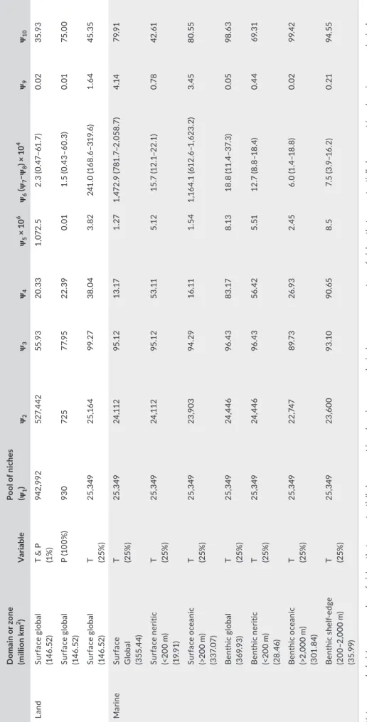
T A B LE 3 C om par is on o f t ot al p seu do -s pe ci es ri chn es s b et w ee n d om ai ns an d e co lo gi ca l z on es D om ai n o r z on e (milli on k m 2) V ar ia ble Po ol o f n ic he s (ψ1 ) ψ2 ψ3 ψ4 ψ5 × 1 0 6 ψ6 (ψ7 –ψ 8 ) × 1 0 4 ψ9 ψ10 La nd Su rf ac e g lo ba l (14 6. 52 ) T & P (1% ) 942 ,9 92 52 7, 44 2 55 .9 3 20 .3 3 1, 07 2. 5 2. 3 ( 0. 47– 61 .7 ) 0.0 2 35 .9 3 Su rf ac e g lo ba l (14 6. 52 ) P ( 10 0% ) 93 0 72 5 77. 95 22 .3 9 0.0 1 1. 5 ( 0. 43 –6 0. 3) 0.0 1 75 .0 0 Su rf ac e g lo ba l (14 6. 52 ) T (25% ) 25, 34 9 25 ,16 4 99 .2 7 38 .0 4 3. 82 24 1. 0 ( 16 8.6 –3 19 .6 ) 1. 64 45 .3 5 M ar ine Su rf ac e G lo ba l (3 55 .4 4) T (25% ) 25, 34 9 24 ,11 2 95 .1 2 13 .17 1. 27 1, 47 2. 9 ( 78 1. 7– 2, 05 8. 7) 4. 14 79 .9 1 Su rf ac e n er iti c (< 20 0 m ) (1 9. 91 ) T (25% ) 25, 34 9 24 ,11 2 95 .1 2 53 .11 5.1 2 15 .7 (1 2.1 –2 2.1 ) 0.7 8 42 .61 Su rf ac e o ce an ic (>2 00 m ) (3 37. 07 ) T (25% ) 25, 34 9 23 ,9 03 94 .2 9 16 .11 1. 54 1,16 4. 1 ( 61 2. 6– 1, 62 3. 2) 3. 45 80 .55 B en th ic g lo ba l (3 69 .9 3) T (25% ) 25, 34 9 24 ,4 46 96 .4 3 83 .17 8.1 3 18.8 (1 1. 4– 37 .3 ) 0.0 5 98 .6 3 B en th ic n er iti c (< 20 0 m ) (2 8. 46) T (25% ) 25, 34 9 24 ,4 46 96 .4 3 56 .42 5. 51 12 .7 (8.8 –1 8. 4) 0.4 4 69 .3 1 B en thi c o ce ani c (> 2, 000 m ) (3 01 .8 4) T (25% ) 25, 34 9 22 ,74 7 89 .7 3 26 .9 3 2. 45 6. 0 ( 1. 4– 18.8 ) 0.0 2 99 .4 2 B en thi c s he lf-ed ge (2 00 −2 ,000 m ) (3 5.9 9) T (25% ) 25, 34 9 23 ,6 00 93 .1 0 90. 65 8. 5 7. 5 ( 3. 9– 16 .2 ) 0. 21 94 .55 N ote : ψ1 : p oo l o f n ic he s, ψ2 : n um be r o f n ic he s t ha t c an p ot en tia lly b e p re se nt i n a d om ai n o r a n e co lo gi ca l z on e, ψ3 : p er ce nt ag e o f n ic he s t ha t c an p ot en tia lly b e p re se nt i n a d om ai n o r a n e co lo gi ca l z on e, PS : p se ud o-sp ec ie s, ψ4 : m ea n n um be r o f p se ud o-sp ec ie s p er n ic he , ψ5 : t ot al n um be r o f p se ud o-sp ec ie s, ψ6, ψ7, ψ8 : m ed ia n ( ψ6 ), a nd f irs t ( ψ7 ) a nd t hi rd ( ψ8 ) q ua rt ile s o f t he a re a ( km 2 ) o cc up ie d b y a p se ud o-sp ec ies , ψ9 : p er ce nt ag e o f t he t ot al a re a o cc up ie d b y a p se ud o-sp ec ie s, ψ10 : s ea so na l s ta bi lit y i n p se ud o-sp ec ie s r ic hn es s, T : t em pe ra tu re , P : p re ci pi ta tio n.
We suggest that the different terrestrial and marine LBGs are caused by water limitation in the subtropics due to high-pressure cells limiting precipitation (Figure 5). These cells cover a more limited area in the Southern Hemisphere, which explains why terrestrial bio-diversity was slightly higher (Figure 2a,d). While high-pressure cells limit terrestrial biodiversity because of their negative influence on precipitation (Figure S2), it is the place where pelagic biodiversity is highest because temperature is the only climatic factor (Figure 2b,e).
Our unifying framework therefore explains why biodiversity peaks at the equator on land, why it peaks at midlatitudes in the epipelagic ocean, and why it is expected to remain high over ner-itic (pelagic and benthic) regions between tropics. In addition, it suggests that deep-sea biodiversity should be little affected by lati-tudes between 40°S and 40°N. We propose that a simple principle, a mathematical constraint on the number of species that can coexist locally, arising from the niche–environment (here climate–environ-ment) interaction, is at the origin of LBGs observed among realms. We have previously called this constraint the chessboard of life (Beaugrand et al., 2018). The rate of net diversification is important because it affects the degree of niche occupancy in a given area. We have shown previously that niche saturation (i.e., the number of occupied niches in an area) was higher in the tropics than in tem-perate systems, probably because of greater net tropical diversifi-cation rates (Dowle, Morgan-Richards, & Trewick, 2013; Jablonski, Roy, & Valentine, 2006) or faster species turnover in extratropical regions (Weir & Schluter, 2007). However, we have also shown that polar systems had the highest degree of niche saturation because the number of niches in polar systems was much lower (Beaugrand et al., 2018). Our results therefore suggest that while speciation is fundamental to fill the chessboard of life, this is not what determines large-scale biodiversity patterns. The arrangement of biodiversity may primarily result from a mathematical constraint that originates from a fundamental interaction: the niche–environment interaction.
4.2 | Total biodiversity comparisons among realms
Modeled total biodiversity was also estimated for each realm and ecological zone at a coarser spatial resolution (Table 3). Spatial pat-terns in pseudo-species richness based on 0.25° × 0.25° and 2° × 2° were highly correlated (r = .99, p < .05, n = 15,929, n*=1), indicating patterns were very close. We first assumed that a niche led to the establishment of only one pseudo-species. With two climatic dimen-sions, the terrestrial domain had greater total pseudo-biodiversity than the marine domain (94 for the terrestrial vs. 0.1 million pseudo-species). Of the 942,992 niches we used (ψ1 in Table 3), 55.93% of the niches led to the establishment of a pseudo-species in the terrestrial domain while between 93.1% and 96.4% of the marine niches (25% of the pool of niches, 25,349) gave a pseudo-species (ψ2 and ψ3 in Table 3). The higher number of terrestrial niches/pseudo-species was caused by the addition of a second climatic dimension.Next, we considered that a niche could lead to the establishment of several pseudo-species provided they were separated spatially
from each other (Buffon's Law; Lomolino et al., 2006); this analysis aimed to reveal the potential influence of allopatric speciation on biodiversity. On average, a terrestrial niche gave 20.3 pseudo-spe-cies when temperature and precipitation were considered, and a marine niche led to between 13.1 and 90.6 pseudo-species at the surface and the shelf-edge, respectively (ψ4, Table 3). Multiplying the number of niches (ψ4) by the mean number of pseudo-species per niche (ψ1) led to the number of pseudo-species expected for each domain or zone (ψ5). The greater number of potential terres-trial niches created higher total pseudo-biodiversity (1,072.5 million terrestrial vs. 23.1 million marine pseudo-species; Aarssen, 1997). The spatial homogeneity of the epipelagic zone means there is less potential for allopatric speciation than in the seabed (ψ4, Table 3), which explains why there are more benthic pseudo-species (ψ5 = 1.3 surface vs. ψ5 = 8.13 million benthic pseudo-species). Similarly, more speciation is likely in the neritic zone, which explains the higher pseudo-biodiversity (Tittensor et al., 2010). The model also predicts the shelf-edge should have a higher total biodiversity than the nerito-benthic zone. Although the shelf-edge zone has been less investigated, a unimodal biodiversity pattern with depth has been suggested with biodiversity peaking between 1,000 m and 3,000 m (Rex, 1981). Because the number of niches was approximately similar among all marine zones (ψ2), it was the potential for allopatric spe-ciation (ψ4) and the area of a realm that most influenced total marine biodiversity (ψ5, Table 3).
High biodiversity is associated with ecosystem stability (Duffy, 2002). However, this should not confer more resistance/ resilience to environmental changes in the terrestrial domain (even though terrestrial total pseudo-biodiversity was higher than marine) because, in our model, the mean spatial range occupied by a terres-trial pseudo-species was lower (ψ6–8 in Table 3); many studies have suggested that species resistance is a function of the area occupied by a species (MacArthur & Wilson, 1967; Thomas et al., 2004). The same also applies for marine zones with a higher total pseudo-bio-diversity, for example, neritic and shelf-edge zones. In terms of per-centage area terrestrial pseudo-species covered the same median area as shelf-edge species (ψ9, Table 3).
Our simulations suggest that spatial heterogeneity increases local biodiversity by enabling the coexistence of more niches and by promoting allopatric speciation (Figure 1 and Table 3). Similarly, monthly stability in pseudo-biodiversity (ψ10, Table 3) was correlated negatively with total pseudo-biodiversity (r = −.67, p = .06, n = 6, log-transformed variables), which suggests that higher temporal het-erogeneity promotes higher biodiversity by enabling more species turnover. The nerito-pelagic zone was characterized by low monthly stability (Table 3), which was due exclusively to temperature. Precipitation, however, was the main cause of terrestrial temporal heterogeneity (Table 3). The deep benthic zone was highly stable.
We scaled pseudo-biodiversity to both catalogued (1,233,500 terrestrial and 193,756 marine species) and estimated (8,740,000 terrestrial and 2,210,000 marine species) eukaryotic biodiversity (Mora et al., 2011). We implemented the model twice: firstly for 930 precipitation niches and secondly for 72 precipitation niches.
Decreasing the number of precipitation niches reduces model accuracy because having fewer niches provides more stepwise transitions but large-scale biodiversity patterns were highly cor-related (r = .92, p < .05, n = 15,929, n*=3), with similar conclusions in terms of niches, biodiversity, and stability (Table 3 vs. Table S2). By decreasing the number of niches, the simulation better ap-proaches nature. With 930 precipitation niches, total terrestrial pseudo-biodiversity—scaled to both catalogued and estimated eukaryotic species—gave 1,397,047 (10,718,238) terrestrial and 30,208 catalogued (231,762 estimated) marine species. Therefore, while this simulation predicted that biodiversity should be higher in the terrestrial than the marine domain, it underestimated cat-alogued biodiversity by factor of 6.4 (catcat-alogued) and 9.53 (es-timated), respectively. When precipitation niches were reduced however (n = 72), total pseudo-biodiversity scaled to catalogued (estimated) species gave 1,111,186 (8,825,091) for the terres-trial domain and 316,069 (2,242,908) for the marine domain. Our model therefore reproduced the difference in observed or esti-mated biodiversity between the marine and terrestrial domains well, although results depended upon the number of selected pre-cipitation niches. Interestingly, our estimate of the deep-sea ben-thic biodiversity (894,881 benben-thic species in areas below 2,000 m and 256,278 in areas between 2,000 m and 200 m) is close to what has been calculated in previous studies (Grassle & Maciolek, 1992; Snelgrove, 1999). Species density is expected to be higher over shelf-edge (200–2,000 m) than deep sea (ψ2-4 in Table S2) but
be-cause the latter realm is larger (301 vs. 36 million km2, Table S2),
there are more total number of species in the deep-sea benthic realm.
In our model, we assumed that dispersal of each pseudo-spe-cies was high enough to fully occupy a given spatial range (i.e., a contiguous area where environmental conditions are suitable for a pseudo-species). In other words, biodiversity patterns were based on the assumption of full distributional range occupancy reached at equilibrium. When the potential for allopatric speciation was con-sidered, the existence of a single barrier to dispersal (i.e., a space with unsuitable environmental conditions in term of temperature or precipitation, or both) was sufficient enough to prevent a species to also occur in another region with suitable environmental conditions, and thereby, another species colonized the area. Because species disperse farther in the oceanic than in the terrestrial realm (Kinlan & Gaines, 2003; Palumbi, 1992), this assumption may have inflated marine biodiversity estimates (and especially seabed biodiversity estimates, see ψ4 in Table 3) and therefore diminished the contrast
of total biodiversity between the terrestrial and the marine realms. Our model did not consider the implications of past climate change to estimate the potential for allopatric speciation. Although this will have no effect on large-scale biodiversity patterns, this may have influenced our estimations of total biodiversity for each realm. This influence would be consistent among realms, however. Consideration of past climate change would reduce the mean num-ber of species per niche in all realms. However, the effect is likely to be more prominent in the terrestrial and in the marine neritic
(benthic and pelagic) realms, less important for the shelf-edge realm, and small for the deep-sea benthic realms.
4.3 | Better understanding of processes influencing
biodiversity
Factors that contribute to the biodiversity are numerous and belong to a large range of temporal and spatial scales (Lomolino et al., 2006). Many authors have made significant attempts to identify the primary factor involved in global biodiversity patterns, and a large number of explanations have been proposed (Allen, Brown, & Gillooly, 2002; Beaugrand et al., 2013; Cardillo, Orme, & Owens, 2005; Colwell & Lees, 2000; Connell & Orias, 1964; Darlington, 1957; Gillooly, Allen, West, & Brown, 2005; Hawkins et al., 2003; Hubbell, 2001; MacAthur, 1965; O'Brien, Field, & Whittaker, 2000; Rohde, 1992; Rosenzweig, 1995; Turner & Hawkins, 2004). Some authors have proposed null or neutral models such as the neutral model of biodiversity and biogeog-raphy (Hubbell, 2001) and the mid-domain effect (Colwell & Hurtt, 1994). Others have suggested that LBGs may originate from the larger area of the tropical belts (Rosenzweig, 1995). Evolutionary explanations have also been put forward (Mittelbach et al., 2007). Perhaps the most compelling hypotheses have been those that invoke an environmental control of biodiversity such as environmental stability or energy availability (Beaugrand, Reid, Ibañez, Lindley, & Edwards, 2002; Rutherford, D'Hondt, & Prell, 1999; Tittensor et al., 2010). Although temperature (both terrestrial and marine realms) and water availability such as pre-cipitation (terrestrial realm) have been often suggested to explain large-scale patterns in the distribution of species (Beaugrand et al., 2010; Lomolino et al., 2006; Rangel et al., 2018; Tittensor et al., 2010), mechanisms by which those parameters control LBGs have remained elusive. More recent findings have suggested an important influence of species’ niche in the generation of patterns of biodiversity (Beaugrand et al., 2013, 2015, 2018; Beaugrand & Kirby, 2018b; Hawkins et al., 2003; Rangel et al., 2018).
Here, we suggest that biodiversity is mathematically constrained by an underlying structure we have previously called the chessboard of life (Beaugrand et al., 2018), which fixes the maximum number of species that can coexist regionally and controls global-scale bio-diversity patterns. Although there are both a large part of contin-gency in biodiversity and species’ occurrence depends upon local stochastic processes (Hubbell, 2001), nature appears ordered and intelligible at a global scale.
We suggest that LBGs are different in the marine and terrestrial realms because of the existence of a second important dimension in the climatic niche of terrestrial species: water availability. (This parameter was estimated in this paper using monthly precipitation.) Although temperature is a key factor in the marine realm (Beaugrand et al., 2010; Rombouts et al., 2009; Tittensor et al., 2010), both temperature and precipitation are needed in the terrestrial realm (Hawkins et al., 2003; Rangel et al., 2018; Whittaker, 1975).
The differential influence of high sea-level pressure cells on cli-mate explains the strong difference observed between LBGs in the terrestrial and marine realms. While high sea-level pressure cells in-fluence positively marine biodiversity through the effect of tempera-ture (mean and temporal variability), they affect negatively terrestrial biodiversity through its adverse effects on precipitation (Figure 5 and Figure S2). Identification of the root mechanisms that explain both LBGs is important because it provides a clue on the primary cause of large-scale biodiversity patterns. High biodiversity can only be observed where the number of niches is high. More niches can be created at the middle part of climatic gradient (either temperature or precipitation). Niche packing, also known as the niche-assembly or the structural theory (MacAthur, 1965; Pellissier, Barnagaud, Kissling, Sekercioglu, & Svenning, 2018; Turner & Hawkins, 2004), resulted here from a mid-domain effect (Colwell & Lees, 2000) in the Euclidean space of the climatic niche (Beaugrand et al., 2013). The number of niches, and thereby the number of species, deeply decreases in areas characterized by extremely low precipitation (Figure S2) and to a lesser degree higher temperature (Figure 3). In the marine realm, the equatorial decrease in biodiversity is due to too high temperature at the equator; see Figure S2 in Beaugrand and colleagues (Beaugrand et al., 2013).
The importance of the second dimension of the climatic niche of terrestrial species (i.e., precipitation) also explains why there are more terrestrial than marine species (Table 3): It increases substan-tially the number of niches (ψ1), diminishes the mean distributional range of a species (ψ6–8), and leads to an increase in potential allopat-ric speciation (ψ4). As a result, terrestrial species have a smaller mean spatial range than marine species (ψ6-8) and the influence of allopat-ric speciation is probably more pronounced (ψ4), exacerbating the contrast between marine and terrestrial biodiversity (ψ5). We have seen previously that our estimations may be affected by dispersal. Because marine dispersal is high in the marine realm (Palumbi, 1992), our estimations of the number of pseudo-species per niche may be too large, although they would reinforce our conclusion on the strong species biodiversity contrast between land and sea.
5 | CONCLUSION
We therefore conclude by stating that a simple principle, a math-ematical constraint on the number of species that can coexist locally, which originates from the niche–environment (here niche-climate) interaction, is at the origin of LBGs and the biodiversity differences observed among realms. Climate has a primordial in-fluence on biodiversity. Mean and spatial gradient in SLP inin-fluence both temperature and precipitation, which have a direct influence on species physiology. Interaction between those parameters and species’ climatic niche generates a mathematical constraint to the maximum number of species that can establish locally, what we called previously the chessboard of life. An additional climatic di-mension in the terrestrial realm (i.e., precipitation), which multi-plies the number of terrestrial niches, may explain why there are
more species in this realm despite the fact that life first emerged in the sea. Spatial heterogeneity may increase biodiversity by allow-ing more niches to coexist and by increasallow-ing allopatric speciation. While speciation is fundamental because it creates species, this process is constrained by the maximum number of niches available locally.
ACKNOWLEDGMENTS
This work was supported by the “Centre National de la Recherche Scientifique” (CNRS), the Research Programme CPER CLIMIBIO (Feder, Nord-Pas-de-Calais), the regional program INDICOP (Nord-Pas-de-Calais), and the ANR project TROPHIK. The authors also thank the French Ministère de l'Enseignement Supérieur et de la Recherche, the Hauts de France Region, and the European Funds for Regional Economic Development for their financial sup-port to this project. We are indebted to Philippe Notez for his help in computer engineering.
CONFLIC T OF INTEREST None declared.
AUTHOR CONTRIBUTION
Gregory Beaugrand: Conceptualization (lead); Data curation (lead); Formal analysis (lead); Funding acquisition (lead); Investigation (lead); Methodology (lead); Project administration (lead); Resources (lead); Software (lead); Supervision (lead); Validation (lead); Visualization (lead); Writing-original draft (lead); Writing-review & editing (lead). Richard Kirby: Writing-original draft (supporting); Writing-review & ed-iting (supporting). Eric Goberville: Data curation (supporting); Wred-iting- Writing-original draft (supporting); Writing-review & editing (supporting). DATA AVAIL ABILIT Y STATEMENT
All data originating from our model are available through a Web site http://metal theory.weebly.com/
ORCID
Gregory Beaugrand https://orcid.org/0000-0002-0712-5223
Richard Kirby https://orcid.org/0000-0002-9867-4454
Eric Goberville https://orcid.org/0000-0002-1843-7855
REFERENCES
Aarssen, L. W. (1997). High productivity in grassland ecosystems: Effected by species diversity or productive species? Oikos, 80, 183– 184. https://doi.org/10.2307/3546531
Allen, P. A., Brown, J. H., & Gillooly, J. F. (2002). Global biodiversity, bio-chemical kinetics, and the energetic-equivalence rule. Science, 297, 1545–1548. https://doi.org/10.1126/scien ce.1072380
Assis, J., Tyberghein, L., Bosh, S., Verbruggen, H., Serrão, E. A., & De Clerck, O. (2017). Bio-ORACLE v2.0: Extending marine data layers for bioclimatic modelling. Global Ecology and Biogeography, 27, 277– 284. https://doi.org/10.1111/geb.12693
Beaugrand, G. (2015a). Marine biodiversity, climatic variability and global
change. London, UK: Routledge.
Beaugrand, G. (2015b). Theoretical basis for predicting climate-in-duced abrupt shifts in the oceans. Philosophical Tansactions of the