Inferences from the vertical distribution of Fe isotopic compositions on pedogenetic processes in soils

HAL Id: hal-00913103

https://hal.archives-ouvertes.fr/hal-00913103

HAL is a multi-disciplinary open access

archive for the deposit and dissemination of sci-entific research documents, whether they are pub-lished or not. The documents may come from teaching and research institutions in France or abroad, or from public or private research centers.

L’archive ouverte pluridisciplinaire HAL, est destinée au dépôt et à la diffusion de documents scientifiques de niveau recherche, publiés ou non, émanant des établissements d’enseignement et de recherche français ou étrangers, des laboratoires publics ou privés.

Inferences from the vertical distribution of Fe isotopic

compositions on pedogenetic processes in soils

Zuzana Fekiacova, Sylvain Pichat, Sophie Cornu, Jérôme Balesdent

To cite this version:

Zuzana Fekiacova, Sylvain Pichat, Sophie Cornu, Jérôme Balesdent. Inferences from the vertical distribution of Fe isotopic compositions on pedogenetic processes in soils. Geoderma, Elsevier, 2013, 209-210, pp.110-118. �10.1016/j.geoderma.2013.06.007�. �hal-00913103�

Inferences from the vertical distribution of Fe isotopic compositions

1

on pedogenetic processes in soils

2

Z. Fekiacova1, S. Pichat2, S. Cornu1 and J. Balesdent1 3

4 5

1

INRA - UR1119 Géochimie des sols et des eaux, Europôle méditerranéen de l'Arbois, F-6

13545 Aix-en-Provence Cedex 04, 7

2

Laboratoire de Géologie de Lyon, Ecole Normale Supérieure de Lyon, Université Claude 8

Bernard, CNRS, UMR 5276, 69007 Lyon, France 9

10

Corresponding author: [email protected] 11

ABSTRACT 1

The isotopic compositions of major elements in soils can help understand the 2

mechanisms and processes that control the evolution of soils and the nature and dynamics of 3

the soil constituents. In this study, we investigated the variations of the Fe concentrations and 4

isotopic compositions combined with classical soil parameters, such as granulometry, pH, 5

and C and N concentrations. We selected three soils submitted to different hydrodynamic 6

functioning along a toposequence: a well-drained Cambisol and two hydromorphic soils, an 7

Albeluvisol and a Gleysol. In the Cambisol, the isotopic variations were small indicating little 8

redistribution of Fe which we attributed to centimetric-scale exchanges from the Si-bound to 9

the weakly-bound iron pools and insignificant subsurface Fe export. In contrast, the 10

hydromorphic soils showed an overall variation of 0.37‰ for 56

Fe (56Fe (‰) = 11

[(56Fe/54Fe)sample/(56Fe/54Fe)IRMM-014 - 1]×1000) and an inverse correlation between the Fe 12

isotopic compositions and the oxide-bound Fe concentrations. We suggest that, in the 13

uppermost horizon, the mobilisation of oxide-bound Fe was due to the reducing conditions 14

and predominantly involved the light Fe isotopes. Similarly, within the Bt horizon of the 15

Albeluvisol, the fluctuations of the water table level induced changes in the redox conditions 16

and thus Fe dissolution and transport of isotopically light Fe. The Fe isotopic composition 17

profile in the B/C horizon of the Gleysol is dominated by the signature of the parental 18

material. Overall, the variations of the underground water table combined with topography-19

driven water flow were suggested to be the main mechanisms of Fe translocation in these 20

hydromorphic soils. Finally, the comparison between Fe isotopes profiles in worldwide soils 21

allow us to show that Fe isotopic variations can help discriminate between various 22

mechanisms and scales of Fe transfer in soils and, accordingly, provide information on the 23

evolution of soils, when used in combination with pedological, geochemical, geographical, 24

and environmental characterisations. 25

Key Words: iron isotopes, soil toposequence, hydromorphy, world soils

1

Highlights

2

 This study investigates the Fe behaviour in three soils along a toposequence. 3

 Fe transport mechanisms were studied using Fe isotopes and classical soil parameters. 4

 In the Cambisol, Fe transfer is limited; in-situ Fe transformations were dominant. 5

 In the hydromorphic soils, the oxide-bound Fe controls the Fe transformations. 6

 Iron isotope ratio variations in soils help distinguish soil evolution processes. 7

1. Introduction

Understanding mechanisms and processes that control soil evolution, the nature and 2

dynamics of major soil constituents and their behaviour in response to natural and 3

anthropogenic changes is among the key scientific challenges in soil research. Iron is one of 4

the major elements in soils. It is released during the alteration of rocks and soils, and 5

participates in mineral neoformation, thereby playing a crucial role in soil differentiation. 6

Iron concentration in soil varies because of different processes: physico-chemical 7

redistributions without transport and short-distance or long-range transport of Fe. In addition, 8

the fate of Fe influences the chemical cycles of other important elements in soils, such as 9

nutrients (e.g. P, Zn) and pollutants (e.g. As, Cd, Zn) (e.g. Anderson and Christensen, 1988; 10

Jacobs et al., 1970; Ramos et al., 1993). Finally, Fe is an essential micronutrients for plants 11

(Marschner, 1995) and human nutrition (WHO, 2002). 12

Stable isotopes analyses have proven to be valuable tools to understand 13

biogeochemical processes in soils (e.g. Fry, 2006). Until the end of the 90’s, these studies 14

were limited to C, N, O, H, and S. However, significant analytical developments over the past 15

years, notably due to the advent of Multi-Collector Inductively-Coupled Plasma Mass-16

Spectrometers (MC-ICP-MS), now allow high-precision analyses required to measure the 17

small isotopic variations of the so-called “non-traditional” stable isotopes that include Fe (e.g. 18

Albarède and Beard, 2004; Dauphas and Rouxel, 2006). Iron has four stable isotopes, 54Fe, 19

56

Fe, 57Fe and 58Fe. The -notation is commonly used to describe the isotopic fractionation 20

relative to the isotopic reference material IRMM-014: XFe (‰) =

21

[(XFe/54Fe)sample/(XFe/54Fe)IRMM-014 - 1]×1000, where X = 56, 57 or 58.

22

In natural environment, 56Fe ranges between -3.5 ‰ and +1.5 ‰ (Beard et al., 23

2003a; Beard and Johnson, 2004; Dauphas and Rouxel, 2006). Igneous rocks represent an 24

isotopically homogeneous terrestrial baseline (56Fe = 0.0 ± 0.05‰) (Beard et al., 2003a), 1

whereas isotopic heterogeneities were initially measured mostly in rivers and lakes, rocks and 2

minerals formed at low temperature, hydrogenous ferromanganese precipitates, pyrites and 3

hydrothermal systems (e.g. Dauphas and Rouxel, 2006; Fantle and DePaolo, 2004). 4

Continental weathering involves processes of mechanical and chemical breakdown of 5

rocks and minerals and subsequent soil development. The parent material, i.e., igneous rocks 6

and clastic sediments, show limited isotopic variations:56Fe = 0.0 ± 0.3‰ (Beard and 7

Johnson, 2004; Fantle and DePaolo, 2004; Johnson et al., 2003). In contrast, soils display a 8

range of variations of the 56Fe from -0.62 to +0.72 ‰ (Emmanuel et al., 2005; Fantle and 9

DePaolo, 2004; Poitrasson et al., 2008; Thompson et al., 2007; Wiederhold et al., 2007a, 10

2007b) indicating that pedogenic processes, leading to soil formation and evolution, generate 11

Fe isotopes fractionations with respect to the parent material. Experimental studies have 12

shown that mineral dissolution results in the preferential liberation of light Fe isotopes into 13

the solution while the residual material becomes accordingly heavier than the parent material 14

(e.g. Beard et al., 1999; Brantley et al., 2004; Wiederhold et al., 2006). In contrast, sorption 15

of Fe(II) onto goethite and mineral ferrihydrite neoformation arising from the abiotic 16

oxidation of aqueous Fe(II) into Fe(III) appears to favour the heavy isotopes (Bullen et al., 17

2001; Icopini et al., 2004). These experimental results have been confirmed by soil studies 18

that show that, in general, the mobile fraction in soils has lighter Fe isotopic composition 19

(Brantley et al., 2004; Fantle and DePaolo, 2004; Thompson et al., 2007; Wiederhold et al., 20

2007a, 2007b). Therefore, the variations of the Fe isotopic signatures in soils can help to 21

investigate the behaviour of Fe in the near-surface environment during pedogenesis and to 22

discriminate between potential processes at the origin of soil evolution. 23

In this study, we investigated both vertical and lateral variations of the Fe 24

concentrations and isotopic compositions combined with the study of classical soil 25

parameters such as granulometry, pH, and C and N concentrations. We used three soil 1

profiles submitted to different hydrodynamic functioning along a toposequence: a well-2

drained oxic profile and two profiles that are waterlogged during a part of the year. The 3

objectives were to (1) study the expression of the isotopic fractionation of iron in these soils, 4

(2) characterize the mechanisms of Fe transport, (3) compare the results with those obtained 5

in previous studies of the Fe isotopes fractionation in soils and (4) evaluate the potential of Fe 6

isotopes to record information about mechanisms of soil transformations. 7

2. Material and methods

2.1. Study area, sampling and soil description 9

The sampling area is located in the Kervidy-Naizin catchment that extends over an 10

area of 4.9 km2 in the centre of Brittany, western France and belongs to the Environment 11

Research Observatory (ERO) AgrHyS (response time in Agro-Hydro Systems). The region is 12

characterised by temperate oceanic climate according to the Köppen climate classification, 13

with a mean annual precipitation of 909 mm and a mean monthly temperature ranging from 14

5.4°C (January) to 17.4°C (August). The land-use is dominated by corn and wheat farming, 15

temporary pastures for dairy production and indoor pig-stock breeding. 16

The soils in this catchment developed from the weathering of the sedimentary 17

Brioverian schist unit (older than 530 Ma) and eolian Quaternary deposits that overlay locally 18

the bedrock (Olivié-Lauquet et al., 2001; Thomas and Le Berre, 2009; Van Vliet-Lanoe et al., 19

1998; Walter and Curmi, 1998). The soils are organised in a toposequence consisting of three 20

soil types: (1) a well-drained, cropped Cambisol (IUSS Working Group WRB, 2006) on the 21

upper part of the slope, characterised by oxic conditions, (2) an Albeluvisol (IUSS Working 22

Group WRB, 2006) at midslope, which represents a transition zone between the well-drained 23

cropland and the poorly drained lowermost part of the landscape and (3) a Gleysol (IUSS 24

Working Group WRB, 2006) developed next to a small creek that flows at the bottom of the 1

slope. The Albeluvisol and Gleysol are planted with poplar trees. Both soils are roughly 2

ploughed every two years to avoid weed growth between the trees (Durand et al., 1998). They 3

both undergo seasonal fluctuations of water saturation, with winter-spring corresponding to a 4

period of reducing chemical conditions while summer, or late summer in the case of the 5

Gleysol, is dominated by oxidative chemical conditions (Davranche et al., 2011; Trolard et 6

al., 2002). The water table in these two soils is located close to the topographic surface 7

(Davranche et al., 2011; Olivié-Lauquet et al., 2001; Pauwels et al., 1996). During rainy 8

periods a temporary water table could develop in the Ap-horizon and lateral drainage could 9

occur. 10

The sampled profiles are located close to the sites C, I and F described by Trolard et 11

al. (2002) for the Cambisol, the Albeluvisol and the Gleysol, respectively. We sampled the 12

soils using an auger with one sample collected every 10 cm respecting the horizons 13

boundaries. 14

In the Cambisol, we sampled the Ap- and B-horizons (Supplementary Table 1). The 15

Ap-ploughing horizon (0 to 20 cm depth) has a silty texture and a dark brown colour 16

(10YR3/1 according to the Munsell chart). The B-horizon (20 to 60 cm depth) has a silty 17

texture and a yellowish-brown colour (10YR5/6). The ratio of 2-20 µm to 20-50 µm fractions 18

is close to one indicating a parent material of eolian origin for the sampled horizons (Walter 19

and Curmi, 1998), likely similar to the loess of northern and/or western Brittany (Haase et al., 20

2007; Le Calvez, 1979). 21

In the Albeluvisol, we sampled the Ap- and Bt-horizons (Supplementary Table 1). 22

The Ap-horizon (0 to 20 cm depth) has a silty texture and a dark-brown to greyish colour 23

(10YR3/2 to 10YR4/2). The Bt-horizon (20 to 60 cm depth) is silty with clay concentration 24

increasing with depth. The ratio of 2-20 µm to 20-50 µm fractions in all the horizons is close 25

to 2 indicating that the soil profile is developed from the sedimentary Brioverian schist parent 1

material (Walter and Curmi, 1998). 2

In the Gleysol, we sampled the Ap- and B/C-horizons (Supplementary Table 1). The 3

Ap-horizon (0 to ~25 cm depth) is dark grey (10YR2.5/1) with a silty-sandy-clayey texture. 4

The illuvial B/C-horizon (~30 to 80 cm depth) is brown to brown-dark yellow (7.5 to 5

10YR4/6) with silty to slightly clayey texture. The ratio of 2-20 µm to 20-50 µm fractions in 6

all the horizons is close to 2 suggesting that the soil mainly developed from the sedimentary 7

Brioverian schist parent material (Walter and Curmi, 1998). 8

The Albeluvisol and Gleysol contain redoximorphic features such as mottling and rust 9

accumulations in root spaces. These features are of millimetric to centimetric size, of brown, 10

yellowish to red or pale grey to greenish colour. They are sparse in the upper Ap horizon but 11

frequently present in the deeper Bt and B/C horizons of the Albeluvisol and Gleysol. 12

2.2. Methods and analyses 13

Collected samples were dried at 40 ºC and sieved to < 2 mm. Aliquots were taken for 14

elemental and isotopic analyses. 15

2.2.1. Fe concentrations: bulk analyses and selective extractions 16

Total iron concentration of the bulk soils was determined on 0.25 g aliquots. Each 17

aliquot was dissolved in a HF-HClO4 mixture after calcination of the organic matter (450 °C).

18

We also used two methods of selective extractions using reducing agents of increasing 19

strength to obtain information about the major pools of iron in the soils studied: (1) the 20

Tamm’s extraction in the dark and (2) the citrate-bicarbonate-dithionite (CBD)-extraction. 21

The Tamm’s reagent is a mixture of oxalic acid and ammonium oxalate (Tamm, 22

1922). The extraction was performed by shaking the sample-solution mixture over 4 hours, at 23

20 °C and in the absence of light with a solid/liquid ratio of 1.25 g/50 ml. This method allows 24

the extraction of weakly bound, poorly crystalline and organic-bound iron (Duchaufour and 1

Souchier, 1966). For the extraction by CBD, the soil sample was exposed to the reactant 2

mixture at 80°C with a solid/liquid ratio of 0.5g/25mL during 30 min. This method extracts 3

the iron bound to oxides and hydroxides (hematite, goethite, lepidocrite) (Mehra and Jackson, 4

1960). 5

Bulk soil iron concentrations and iron concentration in the solutions from the partial 6

extractions were analysed using an Inductively Coupled Plasma-Atomic Emission 7

Spectrometer (LAS Arras). 8

Each extraction was done from an aliquot of the bulk soil. While the Tamm reagent 9

extracts the weakly-bound Fe, the CBD extracts both the weakly bound and the oxide bound-10

Fe. We calculated the oxide-bound Fe concentration by subtracting the weakly-bound Fe 11

measured by Tamm reagent extraction from the CBD extraction and the silicate-bound Fe 12

concentration by subtracting the weakly-bound and the oxide-bound iron from the total iron 13

concentration. 14

2.2.2. Fe isotope ratios measurements 15

Samples for the measurements of Fe isotope ratio were prepared and analysed at the 16

Ecole normale supérieure de Lyon (ENS Lyon), France. An aliquot of each sample was 17

ground using an agate mortar. Approximately 300 mg of sample powder was first treated 18

with 30% H2O2 in order to eliminate the organic matter and then dissolved using a mixture of

19

concentrated HF-HNO3-HCl acids, at ~130°C. Iron was separated and purified by anion

20

exchange chromatography (AG MP1, 100-200 mesh, chloride form). Samples were loaded on 21

the resin in 7N HCl-0.001% H2O2 and Fe was eluted with 2N HCl-0.001% H2O2 (Maréchal et

22

al., 1999). As anion-resins could fractionate Fe isotopes, complete recovery is necessary. The 23

yield was found to be better than 99%. For the iron isotopes ratios measurements, we used a 24

high-resolution MC-ICP-MS (Nu Plasma 1700, Nu Instruments) at ENS Lyon, operated at a 25

mass-resolution (m/Δm) of 3000 ± 100, in dry plasma mode using the Nu DSN desolvation 1

system. Samples were introduced by free aspiration in 0.05N sub-boiled distilled HNO3 using 2

a glass microconcentric nebulizer (uptake rate: 100 μl/min). We used a standard-bracketing

3

approach with IRMM-014 as standard reference material to correct for instrumental mass bias 4

using the exponential law (Albarède and Beard, 2004). Sample measurement solutions were 5

diluted to match the concentration of the IRMM-014 standard within 15%, i.e. 150 to 300 ppb 6

depending on the measurement session. The precision of the isotopic compositions (external 7

reproducibility, 2) calculated on the basis of repeated measurement of the IRMM-014 8

standard were 0.11 and 0.17 ‰ (N= 324) for 56Fe and 57Fe, respectively. In a 57Fe vs. 9

56

Fe diagram, all soil samples measurements plot along a line with a slope of 1.46 10

(Supplementary Fig. 1). This value is equal, within error margins, to the theoretical value of 11

ln(M57/M54)/ln(M56/M54) = 1.487, indicating mass-dependent fractionation and no 12

influence of isobaric interferences. 13

3. Results

The results for the three soil profiles are presented in figures 1 and 2 and in 15

supplementary table 1. Classical soil parameters, such as granulometry, pH, and C and N 16

concentrations, as well as Fe concentrations and isotopic compositions are indicated. The last 17

two sets of results are presented in details in the following sections. 18

3.1. Fe concentration 19

Total iron concentration was found to be uniform along the Ap-B horizons of the 20

Cambisol with only a slight increase at the bottom of the B horizon (Fig. 1). In the 21

Albeluvisol and Gleysol, a sharp decrease (- 330 to 350%) of the total iron concentration in 22

the surface horizons was observed with respect to the deep horizons (Fig. 1b). In the Bt 23

horizon of the Albeluvisol, the iron concentration is maximum around 25 cm depth and 1

decreases slightly below. In the B/C horizon of the Gleysol, the iron concentration increases 2

slightly with depth. In the surface horizons, the Cambisol located at the hilltop had the 3

highest Fe concentration compared to those of the Albeluvisol and Gleysol. The Fe 4

concentrations measured for the three soils were close to those obtained by X-ray 5

fluorescence by Trolard et al. (2002) for nearby locations of the same soil. 6

Selective extractions showed that the contributions of the different Fe pools varied 7

between the horizons and the soil types (Fig. 1c-e and supplementary Table 1). The oxide-8

bound Fe, corresponded to 39 to 81 % of the total iron (Supplementary Fig. 2) and its vertical 9

evolution in each soil mimicked that of the total Fe. 10

The weakly-bound, poorly crystalline iron pool corresponded to 1 to 18 % of the total 11

Fe (Supplementary Fig. 2). It was higher in the Cambisol than in the two other profiles. In the 12

three soils, it increased progressively up to the surface horizon. 13

The silicate-bound Fe represented 18 to 45 % of the total iron (Supplementary Fig. 2) 14

and decreased gradually from depth to surface in the Cambisol. In the Albeluvisol, it 15

increased progressively from a depth of 60 cm to reach a maximum around a depth of 20-30 16

cm, then showed a sharp decrease at the transition between the Bt and the Ap horizons 17

around 20 cm. For the Gleysol, its maximum value was recorded in the deepest sample and 18

decreased progressively to the top of the B/C horizon. A decrease was observed at the B/C – 19

Ap transition. The Ap horizons have similar silicate-bound Fe concentrations in the three 20

profiles. 21

3.2. Fe isotopic compositions 22

The iron isotopic composition in the studied soils varied from 56Fe = -0.15 to 0.26 ‰ 23

(Fig. 2 and supplementary Table 1). The three studied soils show differences in the iron 24

isotopic compositions and variations with depth. The Cambisol profile showed variations of 25

56

Fe from 0.00 to only 0.15 ‰ indicating virtually no vertical fractionation along this 1

profile. In contrast, the amplitude of the Fe isotopic variations was much larger than the 2

external reproducibility within the two other profiles. In the Albeluvisol, 56Fe ranged from 3

0.00 to 0.26 ‰ with a decrease of the 56Fe values from the surface down to ca. 40 cm. In the 4

Gleysol, 56Fe varies from -0.15 to 0.22 ‰ with values decreasing with depth. Notably a 5

marked decrease (-0.19 ‰) was found between the surface Ap horizon and the deeper B/C 6

horizon, corresponding to the observed increase in total Fe concentration (Fig. 1b) and 7

variations in the relative proportions of the various Fe pools (Supplementary Fig. 2). In both 8

the Albeluvisol and the Gleysol, the surface horizons were enriched in heavy Fe isotopes 9

while the deep horizons were enriched in light isotopes (Fig. 2). The non-hydromorphic 10

Cambisol exhibited the lowest 56Fe value and the highest Fe concentration in the surface 11

horizon whereas it was the opposite for the hydromorphic Albeluvisol and Gleysol. 12

4. Discussion

Heterogeneities observed in soils can result from different pedogenetic processes and 14

factors, such as the parent material and topography (Jenny, 1941) that contribute to the soil 15

formation. The soils studied in this work can be differentiated by two main factors: the parent 16

material and the water regime. The Cambisol developed on material of eolian origin under 17

oxic conditions in a well-drained environment. In contrast, the other two soils formed on 18

sedimentary Brioverian schists and remain waterlogged during a great part of the year and are 19

thus subject to reduction processes. The evolution of the Fe behaviour with depth will thus be 20

discussed separately, on the one hand in the Cambisol and on the other hand in the two 21

waterlogged soils in an attempt to identify the mechanisms that control the Fe transfers. 22

4.1. Evolution of the Fe in the Cambisol 23

In the Cambisol, the amount of oxide-bound Fe was found to remain constant, 1

whereas the amount of weakly-bound Fe increased and that of Si-bound Fe decreased from 2

the base to the top of the soil profile (Fig. 1c-e). A question arises about whether an exchange 3

could occur between these last two Fe pools and whether Fe remobilization could take place 4

in this soil profile. The Cambisol profile is characterised by an overall homogeneous bulk Fe 5

isotopic signature (Fig. 2): 56Fe = 0.00 to 0.15‰. Two scenarios could explain this rather 6

uniform isotopic composition: (1) Fe redistribution processes took place but did not 7

fractionate the Fe isotopes or (2) soil evolution processes happened at the centimetric to 8

decimetric scale, i.e. no major vertical Fe translocation occurred in this soil and Fe export out 9

of this soil was extremely limited. In the deepest sample having the highest Si-bound Fe 10

value, the total Fe concentration was 31.1 g kg-1 and the 56Fe was 0.0 ‰. This concentration 11

value is within the range of those of Brittany loess (22.0 ± 17.2 g kg-1 (2σ), Gallet et al. 12

(1998)). In addition, both the concentration and isotopic composition values are, within 13

experimental error, close to those of worldwide loess: [Fetotal] = 22.7 ± 8.8 g kg-1 (Taylor et

14

al., 1983) and 56Fe = 0.05 ± 0.04 ‰ (Beard et al., 2003b). Both observations are in 15

agreement with the fact that the loess is the parent material of the Cambisol (see section 2.1). 16

Mineral weathering by hydrolysis in the surface soil could have liberated Si-bound Fe as 17

indicated by the lower values relative to the rest of the profile (Fig. 1e). The comparison 18

between the average value of the Ap horizon and the deepest sample of the B horizon shows 19

that there is a 4.7 g kg-1 decrease of the total Fe concentration in the surface horizon (Fig. 1b). 20

In addition, in the homogenous Ap-horizon, 4.4 gFe kg-1 is lost from the silicate compartment

21

(Fig. 1e) while 2.2 gFe kg-1 is gained in the weakly-bound Fe pool (Fig. 1d). These

22

observations show that part of the iron is removed from the profile. The loss in the Ap 23

horizon corresponds, however, to a very small decrease of the total Fe concentration (ca. 24

15%) between the deepest sample and the two surface samples of the ploughing horizon. 25

There is also an in-situ transfer from the Si-bound to the weakly-bound iron pool representing 1

about half of the mobilised Fe. To summarize, the redistribution of Fe in the Cambisol was 2

found to be very limited and the net loss of Fe too small to generate significant Fe isotopes 3

fractionation over the Cambisol profile. 4

4.2. Fe transport in the hydromorphic soils (Albeluvisol and Gleysol) 5

The oxide-bound Fe is the dominant pool of Fe in the hydromorphic soils investigated 6

(Fig. 1c and supplementary Fig. 2a). There is a sharp decrease in the oxide-bound Fe 7

concentration in the surface horizons in both soils concomitant with a decrease in total Fe 8

concentration (Fig. 1b, c) suggesting that there is a net export of Fe from these surface 9

horizons. This export can be explained by the presence of a water table that develops in the 10

surface horizons during winter-spring and creates reducing conditions favourable to Fe 11

remobilization. The similarity of both the total Fe concentrations (Fig. 1b) and the isotopic 12

compositions (Fig. 2) in the surface horizons of these soils suggests that the Fe transport in 13

these soils is due to the same process. Dissolution of Fe in the surface horizons would create 14

(1) a decrease in the Fe concentration (Fig. 1b) and (2) a residual Fe pool enriched in heavy 15

isotopes (Fig. 2) because light Fe isotopes are preferentially remobilized by dissolution. The 16

isotopically light product of the dissolution reaction could be transported laterally out of the 17

soil profiles along the topography or vertically to greater soil depth. 18

The iron isotopic composition of the bulk soil is mostly controlled by this process as 19

shown by the strong negative correlation (R2 = 0.70, p < 0.01, data normally distributed) 20

between the 56Fe of the bulk soil samples and the oxide-bound Fe concentration (Fig. 3). 21

Accordingly, the dissolution of Fe-bearing minerals and transport of the free Fe (II) would be 22

the processes that dominate the Fe movements in these hydromorphic soils. 23

By contrast, as aforementioned, there is no relationship between the oxide-bound Fe 1

concentration and the 56Fe value of the bulk soil samples in the Cambisol (Fig. 3). This 2

confirms that the mechanism governing the evolution of Fe in the Cambisol is different from 3

that involved in the Albeluvisol and Gleysol. 4

The Albeluvisol and Gleysol profiles below the Ap horizon are more difficult to 5

interpret. Both soils developed from a sedimentary Brioverian schist parent material (see 6

section 2.1) which is a highly heterogeneous material as shown, in particular, by the complex 7

evolution of the Si-bound iron profiles. Thus, no mass balance calculations could be 8

performed. 9

In the B/C horizon of the Gleysol, the observed overall variation of the Fe isotopic 10

composition with depth is almost an inverse image of the variation of the Si-bound Fe with 11

depth (Figs. 1e and 2). Indeed, there is a strong negative correlation between the 56Fe and 12

the Si-bound concentrations (Supplementary Fig. 3a). This feature could be interpreted as 13

reflecting the imprint of the parental material on the isotopic composition of the Gleysol. 14

Thus, the isotopic composition of the parental material appears to be the main factor that 15

governs the Fe isotopic signature of the B/C horizon of the Gleysol. On the contrary, there is 16

no such relationship in the Bt horizon of the Albeluvisol (Supplementary Fig. 3b). Thus, the 17

parental material has little influence, if any, on the Fe isotopic composition of the Albeluvisol 18

Bt profile. 19

In the Bt horizon of Albeluvisol, the two deepest samples are both enriched in Fe 20

heavy isotopes and depleted in oxide-bound Fe relative to the corresponding Gleysol samples 21

(Figs. 1c and 2). In addition, the Fe concentration profiles (Figs. 1b-e) could reflect a greater 22

dissolution of Fe with increasing depth. Indeed, an underground water table is seasonnaly 23

present in the Bt horizon of the Albeluvisol (see section 2.1; Davranche et al., 2011; Olivié-24

Lauquet et al., 2001; Pauwels et al., 1996). It results in reducing conditions which allow Fe 25

dissolution and the remobilisation of oxide-bound Fe from the flooded horizons of the 1

Albeluvisol. This process favours the removal of light Fe isotopes and leaves a residual Fe 2

pool enriched in heavy isotopes. This is in agreement with the observed negative correlation 3

between the 56Fe of the bulk soil samples and the oxide-bound Fe concentration (Fig. 3). 4

The mobile, isotopically light Fe(II), could be transported down the topography. Thus, the 5

main process that appears to drive the Fe isotopic composition in the Bt horizon of the 6

Albeluvisol is dissolution due to the variation of the level of the underground water table. 7

Our results suggest that both, variation of the underground water level and 8

topography-driven lateral water flows are involved in the translocation of Fe. The 9

isotopically-light Fe removed from the Albeluvisol could be redeposited deeper within the 10

Albeluvisol or in the Gleysol located down the slope or be evacuated from the toposequence. 11

Due to the lack of data on the Fe concentration and isotopic composition on the parent 12

material we have however no clear evidence for such redeposition. This study demonstrates 13

that Fe isotopic compositions can evidence Fe transfers where mass balance calculations are 14

not feasible and pinpoint the factors that control the distribution of Fe within a soil profile. 15

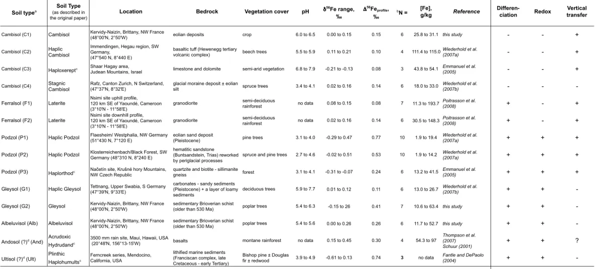
4. 3. Comparison to Fe isotopic compositions in worldwide soils 16

We have compiled published Fe isotope composition of bulk horizons from different 17

soil types (Table 1 and Fig. 4). The overall range for the bulk soil is 56Fe = -0.62 to 0.72 ‰. 18

We have divided the soils into two groups on the basis of the range of their isotopic 19

variations and we have tried to pinpoint the common characteristics for the soils in each 20

group in an attempt to distinguish the factors that control the Fe isotopic fractionations. 21

Group 1 is formed by the soils with small vertical Fe isotopic fractionation, i.e. 22

56

Feprofile≤ 0.15 ‰, with 56Feprofile being the difference between the highest and the lowest

23 56

Fe values in a given profile (Table 1 and Fig. 4). It regroups the Cambisols (56Feprofile = 24

0.08 to 0.15 ‰), the Ferralsols (56Feprofile = 0.08 to 0.14 ‰) and the Haplic Gleysol 1

(56Feprofile = 0.11 ‰). 2

Group 2 consists of soils with significant Fe isotopic fractionation along a vertical 3

profile, such as the Podzols (56Feprofile = 0.24 to 0.77 ‰), the Albeluvisol (56Feprofile = 0.26 4

‰), the Gleysol (56

Feprofile = 0.41 ‰), the Ultisol (56Feprofile = 0.74 %) and the Andosol 5

(56Feprofile = 0.30 ‰). 6

Within group 1, the Cambisols and the Ferralsols develop under oxic and well-drained 7

conditions with a dominant vertical water transfer. Yet, the absence of the Fe isotopic 8

fractionation along the profile suggests that either the water circulation has no effect on the 9

oxidation state of Fe as suggested for Ferralsols by Poitrasson et al. (2008), or that mineral 10

dissolution is not associated with long-distance transfer of Fe and that the released Fe 11

precipitates to form secondary minerals without transport as suggested by Wiederhold et al. 12

(2007a). It is worth noticing that the temporal evolution of the soils does not appear to 13

influence the isotopic signature; indeed, the Cambisols were young, poorly developed soils, 14

whereas the Ferralsols result from a long-term evolution, up to several millions of years 15

(Poitrasson et al., 2008). 16

The Haplic Gleysol and the Stagnic Cambisol show a range of 56Fe variations similar

17

to those of the other profiles of group 1 (56Feprofile< 0.15‰), however, they developed under 18

seasonally or permanently water-saturated, anoxic conditions (Wiederhold et al., 2007b). 19

While reductive Fe mobilization under anoxic conditions was inferred to occur in both soils 20

(Wiederhold et al., 2007b), the absence of large isotopic variations was suggested to indicate 21

that the transport of Fe within each profile was spatially limited and, hence, that most of the 22

Fe would be transformed at the centimetric to decimetric scale. 23

Group 2 of soil profiles correspond to 56Feprofile > 0.15‰ (Table 1 and Fig 4). The 24

Podzols developed under well-aerated conditions with vertical water transfer (Emmanuel et 25

al., 2005; Wiederhold et al., 2007a). Unlike Cambisols from group 1 that evolved in similar 1

settings, the Podzols were characterised by acidic pH. Under these pH conditions, Fe(III) 2

could be dissolved and the released isotopically light Fe could vertically be translocated by 3

organic matter. At depth, isotopically light Fe could precipitate. These processes would result 4

in significant Fe isotopes fractionation. 5

The other soils of group 2 – the Albeluvisol, the Gleysol and the Ultisol – developed

6

under poorly-drained to water-saturated conditions and were subject to variations of the redox 7

conditions due to changes in water-saturation states. In all cases, the reductive dissolution of 8

Fe would affect preferentially the light isotopes which become mobile. Hence, the residual 9

material would become isotopically heavier, while the levels where Fe accumulation occurred 10

would become enriched in isotopically light Fe. 11

The Andosol has an intermediate behaviour between the Podzols and the water-12

saturated soils. It formed along volcanic slope in Hawaii with a mean annual precipitation of 13

3500 mm/year. Water-saturated (Thompson et al., 2007) and low oxygen availability (Schuur 14

et al., 2001) conditions would take place during the periods of higher precipitation. Iron 15

isotope fractionation would result from the reductive dissolution of Fe, and δ56Fe values 16

would increase with increasing removal of Fe. 17

To conclude, iron isotopes represent a great tool for studying the mechanisms and 18

scales (centimetric- to toposequence-) of Fe transfer in soils and distinguishing between 19

various mechanisms of soil evolution. For these reasons, they should be used in combination 20

with pedological and geochemical characterisation as well as an appropriate characterisation 21

of the geographical and environmental contexts. 22

5. Conclusions

Iron isotopes profiles in soils have been shown to be a tool of great potential to better 1

understand the fate of Fe in soils and the evolution of soils. In this study, iron isotopic 2

variations have helped us to distinguish between various mechanisms of Fe transport within a 3

soil profile and along a toposequence. 4

For the Cambisol, Fe isotopic fractionations were small and Fe transfers were limited. 5

The mechanisms corresponding to these observations were: (1) centimetric to decametric-6

scale exchanges between iron pools and (2) lateral transport of Fe down the slope; the latter 7

representing only a small proportion of the total Fe. 8

The bulk Fe isotopic composition in the hydromorphic soils (Albeluvisol and Gleysol) 9

was found to be dominated by the behaviour of the oxide-bound Fe. In the surface horizon, 10

the main mechanism of Fe transport in these soils is a strong Fe dissolution and transport of 11

isotopically light Fe out of these horizons. Even if Fe could be transferred within each profile, 12

it would mainly be transported laterally along the slope. The fluctuations of the underground 13

water level could also induced the translocation of Fe after dissolution of the oxides during 14

the periods of reducing conditions corresponding to the high level stands. Iron isotopic 15

compositions have allowed us to show that this phenomenon is dominant in the Bt horizon of 16

the Albeluvisol. Finally, Fe isotopic composition of the B/C horizon of the Gleysol is 17

dominated by the signature of the parental material. 18

Iron isotopic compositions have allowed us to (1) distinguish between the in-situ 19

processes (centimetric- to decimetric-scale) and the processes inducing Fe transfer at the 20

profile- and toposequence-scale, and (2) identify the mechanisms or factors that control the 21

Fe distribution in soils. Consequently, determining the Fe isotopic compositions represents a 22

powerful tool for studying the fate of Fe in soil systems when no sufficient data are available 23

for full mass balance calculations. 24

More generally, the comparison we made of Fe isotopes profiles in various soils of the 1

world shows that Fe isotope ratio variations along a soil profile are linked to the evolution 2

processes that have affected the soil. Hence, Fe isotopic compositions in soils can help us 3

discriminate between various mechanisms of soil evolution when they are used in 4

combination with pedological, geochemical, geographical, and environmental

5

characterisations. 6

Acknowledgements 1

We thank the team of the environmental research observatory (ORE) AgHrys (Response time 2

for hydro-chemical fluxes to the evolution of Agro-Hydro Systems) for providing access to 3

their sampling site, Fabienne Trolard for her help with the sampling, Philippe Télouk for his 4

help with the Nu1700 MC-ICP-MS measurements at the ENS Lyon, Chantal Douchet, 5

Emmanuelle Albalat, and Florent Arnaud-Godet for the maintenance of the clean lab at the 6

ENS Lyon, and Jan Wiederhold for his comments on an early version of this manuscript. We 7

also thank the editor (O.K. Borggaard) and an anonymous reviewer for their detailed and 8

constructive reviews. We thank the INRA for financial support for this project. SP was 9

supported by the CNRS Institut National des Sciences de l’Univers (Interrvie AO 2010) and 10

the Ecole Normale Supérieure de Lyon. 11

Figure Captions 1

Fig. 1. Variations of the soil characteristics with depth in the three studied soil profiles. (a) 2

clay concentration, (b) total Fe concentration, (c) oxide-bound Fe extracted with CBD, (d) 3

weakly-bound Fe extracted with Tamm’s reagent, and (e) calculated Si-bound Fe (see the 4

Material and Methods section for details). The vertical dashed line in (b) represents the 5

average Fe concentration (50.5 g kg-1) for the Bt and B/C horizons of the Albeluvisol and 6

Gleysol, (see section 4.2 for details). 7

Fig. 2. Variations of the iron isotopic compositions (56Fe) with depth in the three studied 8

soil profiles. 9

Fig. 3. Relationship (black line) between the bulk iron isotopic compositions and the oxide-10

bound Fe concentration in the Albeluvisol and the Gleysol. There is no relationship for the 11

Cambisol. 12

Fig. 4. Global patterns of bulk Fe isotope ratio variations in the Naizin soils and other soils 13

worldwide. Two behaviours are distinguished: soil profiles with limited 56Fe variations 14

(goup 1), and soils in which significant 56Fe variations were measured (group 2). The details 15

for each soil are indicated in Table 1. 16 17 18 19 20 21

References 1

Albarède, F., Beard, B.L., 2004. Analytical methods for non-traditional isotopes, in Johnson, 2

C.M., Beard, B.L., Albarède, F. (Eds.), Geochemistry of Non-Traditional Stable 3

Isotopes. Rev. Mineral. Geochem. 55, pp. 113-152. 4

Anderson, P.R., Christensen, T.H., 1988. Distribution coefficients of Cd, Co, Ni, and Zn in 5

soils, J. Soil Sci. 39, 15-22. 6

Beard, B.L., Johnson, C.M., 2004. Fe Isotope Variations in the Modern and Ancient Earth 7

and Other Planetary Bodies, in Johnson, C.M., Beard, B.L., Albarède, F. (Eds.), 8

Geochemistry of Non-Traditional Stable Isotopes. Rev. Mineral. Geochem. 55, pp. 9

319-357. 10

Beard, B.L., Johnson, C.M., Cox, L., Sun, H., Nealson, K.H., Aguilar, C., 1999. Iron isotope 11

biosignatures. Science 285, 1889-1892. 12

Beard, B.L., Johnson, C.M., Skulan, J.L., Nealson, K.H., Cox, L., Sun, H., 2003a. 13

Application of Fe isotopes to tracing the geochemical and biological cycling of Fe. 14

Chem. Geol. 195, 87-117. 15

Beard, B.L., Johnson, C.M., Von Damm, K.L., Poulson, R.L., 2003b. Iron isotope constraints 16

on Fe cycling and mass balance in oxygenated Earth oceans, Geology 31, 629-632. 17

Brantley, S.L., Liermann, L., Guynn, R.L., Anbar, A.D., Icopini, G.A., Barling, J., 2004. Fe 18

isotopic fractionation during mineral dissolution with and without bacteria. Geochim. 19

Cosmochim. Acta 68, 3189-3204. 20

Bullen, T.D., White, A.F., Childs, C.W., Vivit, D.V., Schulz, M.S., 2001. Demonstration of 21

significant abiotic iron isotope fractionation in nature. Geology 29, 699-702. 22

Dauphas, N., Rouxel, O., 2006. Mass spectrometry and natural variations of iron isotopes. 23

Mass Spectrom. Rev. 25, 515-550. 24

Davranche, M., Grybos, M., Gruau, G., Pédrot, M., Dia, A. and Marsac, R. 2011. Rare earth 25

element patterns: A tool for idnentifying metal sources during wetland soil reduction. 1

Chem Geol. 284, 127-137. 2

Duchaufour, P., Souchier, B., 1966. Note sur une méthode d’extraction combinée de 3

l’aluminium et du fer libres dans les sols. Science du sol 1, 17-29. 4

Durand, P., Henault, C., Bidois, J., Trolard, F., 1998. La dénitrification en zone humide de 5

fonds de vallée, in: Cheverry, C. (Ed), Agriculture intense et qualité des eaux. INRA 6

Editions, Paris, pp. 223-231. 7

Emmanuel, S., Erel, Y., Matthews, A., Teutsch, N., 2005. A preliminary mixing model for Fe 8

isotopes in soils. Chem. Geol. 222, 23-34. 9

Fantle, M.S., DePaolo, D.J., 2004. Iron isotopic fractionation during continental weathering. 10

Earth Planet. Sci. Lett. 228, 547-562. 11

Fry, B., 2006. Stable isotope ecology, Springer, New York, pp 308. 12

Gallet, S., Jahn, B., Van Vliet-Lanoe, B., Dia, A. and Rossello, E., 1998. Loess geochemistry 13

and its implications for particle origin and composition of the upper continental crust. 14

Earth and Planetary Science Letters, 156: 157-172. 15

Haase, D., Fink, J., Haase, G., Ruske, R., Pécsi, M., Richter, H., Altermann, M. and Jäger, 16

K.-D. 2007. Loess in Europe - its spatial distribution based on a European Loess Map, 17

scale 1:2,500,000. Quaternary Science Reviews 26, 1301-1312. 18

Icopini, G.A., Anbar, A.D., Ruebush, S.S., Tien, M., Brantley, S.L., 2004. Iron isotope 19

fractionation during microbial reduction of iron: the importance of adsorption. 20

Geology 32, 205-208. 21

IUSS Working Group WRB, 2006. World Reference Base for Soil Resources 2006, World 22

Soil Resources Rep. 103, second ed. FAO, Rome. 23

Jacobs, L.W., Syers, J.K., Keeney, D.R., 1970. Arsenic Sorption by Soils, Soil Sci. Soc. Am. 24

J. 34, 750-754. 25

Jenny, H. 1941. Factors of soil formation. Dover Publications, New York, pp. 191. 1

Johnson, C., Beard, B., Beukes, N., Klein, C., O'Leary, J., 2003. Ancient geochemical cycling 2

in the Earth as inferred from Fe isotope studies of banded iron formations from the 3

Transvaal Craton. Contrib. Mineral. Petrol. 144, 523-547. 4

Le Calvez, L., 1979. Genèse des formations limoneuses de Bretagne centrale: essai de 5

modélisation. Ph. D. thesis, Université de Rennes I. 6

Maréchal, C.N., Télouk, P. and Albarède, F., 1999. Precise analysis of copper and zinc 7

isotopic compositions by plasma-source mass spectrometry. Chemical Geology 156, 8

251-273. 9

Marschner H., 1995. Mineral nutrition of higher plants. Academic Press, London, pp 889. 10

Mehra, O.P., Jackson, M.L., 1960. Iron oxide removal from soils and clays by a dithionite-11

citrate system buffered with sodium bicarbonate. Clays Clay Miner. 7, 317-327. 12

Olivié-Lauquet, G., Gruau, G., Dia, A., Riou, C., Jaffrezic, A. and Henin, O. 2001. Release of 13

trace elements in wetlands: role of seasonal variability. Water Research 35, 943-952. 14

Pauwels ., artelat A., Foucher . , achassagne . 1996. D nitrification dans les eaux 15

souterraines du bassin versant du oet Dan Suivi g ochimi ue et hydrog ologi ue 16

du processus. Rapport BRGM R39055, 66 p., 23 fig., 6 tab. 17

Poitrasson, F., Viers J., Martin, F., Braun, J.J., 2008. Limited iron isotope variation in recent 18

lateritic soils from Nsimi Camerron: Implications for the global Fe geochemical cycle. 19

Chem. Geol. 253, 54-63. 20

Ramos, L., Hernandez, L.M., Gonzalez, M.J., 1993. Sequential Fractionation of Copper, 21

Lead, Cadmium and Zinc in Soils from or near Donana National Park, J. Environ. 22

Qual. 23, 50-57. 23

Schuur, E. A. G. 2001 The Effect of Water on Decomposition Dynamics in Mesic to Wet 24

Hawaiian Montane Forests. Ecosystems 4, 259-273. 25

Schuur, E.A., Chadwick, O.A., Matson, P.A., 2001. Carbon cycling and soil carbon storage in 1

mesic to wet Hawaiian montane forests. Ecology 82, 3182-3196. 2

Tamm, O., 1922. Eine Method zur Bestimmung der anorganishen Komponenten des 3

Golkomplex in Boden. Medd. Statens skogforsoksanst 19, 385-404. 4

Taylor, S.R., McLennan, S.M., McCulloch, M.T., 1983. Geochemistry of loess, continental 5

crustal composition and crustal model ages, Geochim. Cosmochim. Acta 47, 1897-6

1905. 7

Thomas, E. Le Berre, P., 2009. Carte géol. France (1/50 000), feuille Josselin (350). Orléans: 8

BRGM. Notice explicative par Thomas, E., Le Berre, P., avec la collaboration de 9

Foucuad-Lemercier B., Le Bris, A.-L., Carn-Dheilly, A., Naas, P. (2009), 90 pp. 10

Thompson, A., Ruiz, J., Chadwick, O.A., Titus, M., Chorover, J., 2007. Rayleigh 11

fractionation of iron isotopes during pedogenesis along a climatic sequence of 12

Hawaiian basalts. Chem. Geol. 238, 72-83. 13

Trolard, F., Jaffrezic, A., Bourrié, G. and Robin, P. 1999. Pollution diffuse en zone 14

d'agriculture intensive. INRA USARQ, Rennes, p. 46. 15

Trolard, F., Bourrié, G., Jaffrezic, A. 2002 Distribution spatiale et mobilité des ETM en 16

région d’élevage intensif, in Baize, D., Tercé, M. (Eds.), Les éléments traces 17

métalliques dans les sols. Approches fonctionnelles et spatiales. INRA Paris, pp 183-18

199. 19

Van Vliet-Lanoe, B., Pellerin, J., Chauvel, J.J., 1998. Le bassin du Coët-Dan au coeur du 20

massif armoricain. 1. Le cadre géologique et géomorphologique, in Cheverry, C. 21

(Ed.), Agriculture intense et qualité des eaux. INRA Editions, Paris, pp. 11-16. 22

Walter, C. and Curmi, P., 1998. Les sols du bassin versant du Coët-Dan: organisation, 23

variabilité spatiale et cartographie, in Cheverry, C. (Ed.), Agriculture intense et qualité 24

des eaux. INRA Editions, Paris, pp. 85-105. 25

WHO (World Health Organization), 2002. The world health report: reducing risks, promoting 1

healthy life, www.who.int/whr/2002/en/index.html 2

Wiederhold, J.G., Kraemer, M., Teutsch, N., Borer, P.L., Halliday, A.N., Kretzschmar, R., 3

2006. Iron isotope fractionation during proton-controlled and reductive dissolution of 4

goethite. Environ. Sci. Technol. 40, 3787-3793. 5

Wiederhold, J.G., Teutsch, N., Kraemer, M., Halliday, A.N., Kretzschmar, R., 2007a. Iron 6

isotope fractionation in oxic soils by mineral weathering and podzolization. Geochim. 7

Cosmochim. Acta 71, 5821-5833. 8

Wiederhold, J.G., Teutsch, N., Kraemer, M., Halliday, A.N., Kretzschmar, R., 2007b. Iron 9

isotope fractionation during pedogenesis in redoximorphic soils. Soil Sci. Soc. Am. J. 10

71, 1840-1850. 11

a 0 20 40 60 Total Fe, g/kg 0 1 2 3 4 Weakly bound-Fe, g/kg 0 20 40 Oxide bound-Fe, g/kg 0 10 20 Si-bound Fe, g/kg 0 10 20 30 40 50 60 70 80 100 200 300 Depth, cm Clay, g/kg Cambisol Albeluvisol Gleysol b c d e Figure 1

0 10 20 30 40 50 60 70 80 -0.2 -0.1 0.0 0.1 0.2 0.3 Depth (cm) b56 Fe (‰) Cambisol Albeluvisol Gleysol 2m Figure 2

y = -0.01x + 0.25 R2 = 0.69 -0.20 -0.10 0.00 0.10 0.20 0.30 0 10 20 30 40 50 60

b

Fe, ‰

oxide-bound Fe, g/kg

b56 Fe, ‰ Cambisol (C1) Cambisol (C2) Cambisol (C3) 0 20 40 60 80 100 Depth, cm Podzol (P1) Podzol (P2) Podzol (P3) 0 5 10 15 20 25 Depth, m Ferralsol (F1) Ferralsol (F2) 0 10 20 30 40 50 60 Depth, cm Albeluvisol (Alb) 0 20 40 60 80 100 120 140 Haplic Gleysol (G1) 0 10 20 30 40 50 60 70 80 90 0 10 20 30 40 50 60 70 Gleysol (G2) 0 20 40 60 80 100 120 140 Depth, cm Ultisol (Ult) b56 Fe, ‰ b56 Fe, ‰ b56 Fe, ‰ Andosol (And) b56 Fe, ‰ b56 Fe, ‰ Well-drained conditions, vertical water transfer

Poorly-drained conditions, lateral water transfer or no transfer 0 20 40 60 80 100 120 140 Depth, cm b56 Fe, ‰ Stagnic Cambisol (C4) 0 10 20 30 40 50 60 70 80 90 -0.64 -0.32 0.00 0.32 0.64 Depth, cm -0.64 -0.32 0.00 0.32 0.64 -0.64 -0.32 0.00 0.32 0.64 -0.64 -0.32 0.00 0.32 0.64 -0.64 -0.32 0.00 0.32 0.64 -0.64 -0.32 0.32 0.64 -0.64 -0.32 0.00 0.32 0.64 0.00 GROUP 2: 656 Fe profile > 0.15‰ GROUP 1: 656 Fe profile < 0.15‰ b56 Fe, ‰ -0.64 -0.32 0.00 0.32 0.64

Soil typea

Soil Type (as described in the original paper)

Location Bedrock Vegetation cover pH 56Fe range,

‰

56 Feprofile,

‰ b

N = [Fe],_g/kg Reference Differen-_ciation Redox _transferVertical

Cambisol (C1) Cambisol Kervidy-Naizin, Brittany, NW France

(48°00'N, 2°50'W) eolian deposits crop 6.0 to 6.5 0.00 to 0.15 0.15 6 25.8 to 31.1 this study - - +

Cambisol (C2) Haplic

Cambisol

Immendingen, Hegau region, SW Germany,

(47°540 N, 8°440 E)

basaltic tuff (Hewenegg tertiary

volcanic complex) beech trees 5.5 to 5.9 0.11 to 0.21 0.10 4 111.4 to 115.0

Wiederhold et al.

(2007a) - - +

Cambisol (C3) _Haploxereptc Shaar Hagay area,

Judean Mountains, Israel limestone and dolomite semi-arid vegetation 6.8 to 7.9 -0.21 to -0.13 0.08 3 43.8 to 54.1

Emmanuel et al.

(2005) - - +

Cambisol (C4) Stagnic

Cambisol

Rafz, Canton Zurich, N Switzerland, (47°37'N, 8°32'E)

glacial moraine deposit ± eolian

silt spruce trees 3.4 to 4.1 0.02 to 0.16 0.14 6 18.0 to 33.0

Wiederhold et al.

(2007b) - -

-Ferralsol (F1) Laterite

Nsimi site uphill profile,

120 km SE of Yaoundé, Cameroon (3°10'N - 11°58'E) granodiorite semi-deciduous rainforest no data 0.08 to 0.15 0.08 7 11.3 to 193.7 Poitrasson et al. (2008) + - + Ferralsol (F2) Laterite

Nsimi site downhill profile, 120 km SE of Yaoundé, Cameroon (3°10'N - 11°58'E) granodiorite semi-deciduous rainforest no data 0.02 to 0.16 0.14 6 30.5 to 148.3 Poitrasson et al. (2008) + - +

Podzol (P1) Haplic Podzol Flaesheim/ Westphalia, NW Germany

(51°430 N, 7°120 E)

eolian sand deposit

(Pleistocene) pine trees 3.1 to 4.0 -0.29 to 0.47 0.77 10 1.9 to 19.4

Wiederhold et al.

(2007a) + + +

Podzol (P2) Haplic Podzol Klosterreichenbach/Black Forest, SW

Germany (48°310 N, 8°240 E)

hematitic sandstone (Buntsandstein, Trias) reworked by periglacial processes

spruce and pine trees 2.7 to 4.6 -0.02 to 0.51 0.53 10 1.9 to 14.2 Wiederhold et al.

(2007a) + + +

Podzol (P3) _Haplorthodc Na etín site, Kru né hory Mountains, NW Czech Republic

quartzite and biotite - sillimanite

gneiss forest 3.1 to 4.1 -0.31 to -0.07 0.24 6 13.2 to 41.5

Emmanuel et al.

(2005) + + +

Gleysol (G1) Haplic Gleysol Tettnang, Upper Swabia, S Germany

(47°39'N, 9°33'E)

carbonates - sandy sediments (Pleistocene) + a layer of loamy sediments

deciduous trees 5.9 to 7.7 0.01 to 0.12 0.11 6 13.0 to 26.7 Wiederhold et al. _(2007b) + +

-Gleysol (G2) Gleysol Kervidy-Naizin, Brittany, NW France

(48°00'N, 2°50'W)

sedimentary Brioverian schist

(older than 530 Ma) poplar trees 5.4 to 6.3 -0.15 to 26 0.41 7 10.6 to 63.4 this study + +

-Albeluvisol (Alb) Albeluvisol Kervidy-Naizin, Brittany, NW France

(48°00'N, 2°50'W)

sedimentary Brioverian schist

(older than 530 Ma) poplar trees 5.4 to 5.6 0.00 to 0.26 0.26 6 11.7 to 52.7 this study + +

-Andosol (?)d _(And) Acrudoxic

Hydrudandc

3500 mm rain site, Maui, Hawaii, USA

(20°48'N, 156°13-15'W) basalts montane rainforest no data 0.15 to 0.45 0.30 4 54.3 to 97

Thompson et al. (2007) Schuur (2001)

+ + ?

Ultisol (?)d _(Ult) Plinthic

Haplohumultsc

Ferncreek series, Mendocino, California, USA

lithified marine sediments (Franciscan complex, late Cretaceous - early Tertiary)

Bishop pine ± Douglas

fir ± redwood 3.9 to 4.9 -0.61 to 0.13 0.74 3 no data

Fantle and DePaolo

(2004) + +

-a _{Soil type as translated to WRB using the information available. In Fig. 4, soils are referred to as using this denomination.} b

N is the number of data points in each profile

c_{Soil Taxonomy}

d_{No sufficient information is available to assign a precise WRB denominantion.}

Table 1: Compilation of bulk Fe isotopic compositions in worldwide soil profiles and characteristics of these soils. e