A simple test for the ignorability of non-compliance in experiments

(1)

A simple test for the ignorability of non-compliance in experiments

Martin Huber

June 3, 2013

University of St. Gallen, Dept. of Economics

Abstract: This paper proposes a simple method for testing whether non-compliance in experiments is

ignorable, i.e., not jointly related to the treatment and the outcome. The approach consists of (i) regressing

the outcome variable on a constant, the treatment, the assignment indicator, and the treatment/assignment

interaction and (ii) testing whether the coefficients on the latter two variables are jointly equal to zero. A

brief simulation study illustrates the finite sample properties of the test.

Keywords: experiment, treatment effects, non-compliance, endogeneity, test.

JEL classification: C12, C21, C26.

Address for correspondence: Martin Huber, SEW, University of St. Gallen, Varnb¨uelstrasse 14, 9000 St. Gallen,

(2)

1 Introduction

Non-compliance in experiments arises if some units receive a treatment different to the random

assignment. While the average treatment effect (ATE) on the subgroup of compliers (whose

treatment complies with the assignment) is identified under some conditions, one typically prefers

to make causal statements for the entire experimental population. In general, however, the ATEs

on compliers and the entire population are only equivalent if non-compliance is ignorable, implying

that compliers and non-compliers are comparable in terms of unobservables affecting the outcome.

Given that the assignment is random, does not directly affect the outcome, and influences the

treatment, the ignorability of non-compliance has a testable implication: The assignment must

be independent of the outcome conditional on the treatment. Conversely, if non-compliance is

non-ignorable and causes treatment confounding, conditioning on the latter generally introduces

dependence between the assignment and outcome. We propose testing ignorability by (i)

regress-ing the outcome on a constant, the treatment, the assignment, and the treatment/assignment

interaction and (ii) jointly testing for zero coefficients on the latter two variables.

A conceptual extension is testing conditional ignorability given observed covariates, for which

de Luna and Johansson (2012) proposed a nonparametric method. Donald, Hsu, and Lieli (2011)

suggest a further test requiring one-sided non-compliance (no unit randomized out gets the

treat-ment) under which the ATE on the treated compliers corresponds to that on all treated. This

pa-per focuses on unconditional ignorability, but conditional testing is straightforward if covariates

are discrete (by testing within cells of covariate values or based on a fully interacted regression

model). Section 2 discusses the model and testing, Section 3 presents a simulation study.

2 Model and testing

We are interested in the ATE of a binary treatment D on an outcome Y . In experiments, the

(3)

non-compliance, Z 6= D for a subgroup of units, implying that D is not a deterministic function

of Z. We consider the following general models for Y and D:

Y = g(D, U ), (1)

D = I{h(Z, V ) ≥ 0}. (2)

g and h denote unknown functions, U and V are unobserved terms in the outcome and treatment

equations, and I{·} is the indicator function. To give an example, Z may be random assignment

to a training program, D actual program participation, Y earnings after assignment, and V and

U unobserved measures of motivation to take the treatment and at work, respectively.

To translate our model into the potential outcomes framework, see for instance Rubin (1974),

denote by Y (d) the potential outcome when setting the treatment to d and by D(z) the potential

treatment when setting the assignment to z, with d, z ∈ {0, 1}. Exogenously fixing d, z in (1)

and (2) yields the potential outcomes and treatments:

Y (d) = g(d, U ), (3)

D(z) = I{h(z, V ) ≥ 0}. (4)

If V affects D conditional on Z, non-compliance exists and D(z) 6= z for some units. Furthermore,

if V and U are associated as it appears plausible in our example with unobserved motivation,

non-compliance is non-ignorable and D is confounded by U .

We now discuss assumptions under which the independence of V and U , which implies the

ignorability of non-compliance, can be tested if data sampling is i.i.d.

Assumption 1: Z⊥(U, V ).

‘⊥’ denotes independence. Along with our model, Assumption 1 implies that Z is randomly

assigned (by its independence of V ) and does not have a direct effect on Y (by its independence

(4)

potential outcomes and treatment states: Z⊥{Y (1), Y (0), D(1), D(0)}.

Assumption 2: Z and D are not independent.

In experiments, Assumption 2 appears reasonable because assignment should affect the treatment

of some units, for which I{h(1, V ) ≥ 0} 6= I{h(0, V ) ≥ 0} or equivalently, D(1) 6= D(0). Those

whose treatment reacts to the assignment are either compliers (D(1) = 1 and D(0) = 0) or

defiers (D(1) = 0 and D(0) = 1). In contrast, the treatment states of always takers (D(1) = 1

and D(0) = 1) and never takers (D(1) = 0 and D(0) = 0) are not affected by the assignment.

To identify the complier ATE, Angrist, Imbens, and Rubin (1996) assume compliers (Pr(D(1) >

D(0)) > 0) but rule out defiers (Pr(D(1) ≥ D(0)) = 1), which is a special case of Assumption 2.

Our third assumption states that non-compliance is ignorable. This is the restriction to be

tested, conditional on the satisfaction of Assumptions 1 and 2.

Assumption 3: V ⊥U .

Assumptions 1 and 3 together imply that D⊥U or in terms of potential outcomes, that D⊥Y (d).

I.e., the treatment only randomly deviates from the assignment so that the distribution of U (or

Y (d)) is equal among compliers and in the entire population. If Assumption 2 holds, too, we

obtain the following testable implication:

Z⊥Y |D. (5)

To see this, note that Assumptions 1 and 2 are not sufficient for (5): If D is associated with Z

(Assumption 2), then Z⊥U |D (or Z⊥Y |D) does not necessarily hold even if Z⊥Y (Assumption

1). Because if U is related to V and thus confounds D, conditioning on the latter introduces a

dependence between Z and Y , even though the true effect of Z on Y is zero due to Assumption

1. However, if we impose Assumption 3, also D⊥U such that Z⊥U |D, which implies Z⊥Y |D by

our model. Therefore, Assumption 3 can be tested by verifying (5).

Figure 1 graphically presents our model both with and without Assumption 3, where each

(5)

Figure 1: Directed acyclical graphs under independence (a) and dependence (b-d) of U, V

In (a), Assumptions 1 to 3 are satisfied and conditioning on D does not entail dependence between

Z and U (or Y (d)). In (b), (c), and (d), however, Assumption 3 is violated due to dependence

between V and U . Therefore, conditioning on D introduces an association between U and Z (and

thus, Y (d) and Z).

For testing (5), we suggest to (i) regress Y on a constant, D, Z, and the interaction D · Z (and

to compute robust standard errors if heteroskedasticity should be allowed for) and (ii) jointly

test whether the coefficients on Z and D · Z are equal to zero by a Wald or F-test. Using OLS

regression, this amounts to testing whether E(Y |D = 0, Z = 0) = E(Y |D = 0, Z = 1) (reflected

by the coefficient on Z) and E(Y |D = 1, Z = 1) = E(Y |D = 1, Z = 0) (reflected by the sum

of coefficients on Z and D · Z), because the model is fully saturated. This is an unconditional

version of de Luna and Johansson (2012), who nonparametrically test for equalities in means given

observed covariates. However, note that mean independence is necessary, but not sufficient for

(5), postulating full independence between Z and Y given D. Instead of OLS, quantile regression

may therefore be used to test general distributional features. On the other hand, if one is solely

interested in ATEs (rather than quantile treatment effects), mean independence suffices for the

innocuousness of non-compliance and we will henceforth focus on this case.

To see why testing verifies the ignorability of non-compliance, let T ∈ {a, c, ¯d, n} be the

compliance type, where a denotes the always takers, c the compliers, ¯d the defiers, and n the

never takers. Any E(Y |D = d, Z = z) with d, z ∈ {0, 1} consists of a mixture of mean potential

outcomes of (at most) two types. E.g., an observation with D = 1, Z = 1 implies that D(1) = 1

and may thus either be a complier or an always taker. However, as the counterfactual treatment

under Z = 0 is unknown, the exact type cannot be determined. Denote by E(Y (d)|T = t)

(6)

particular type in the population. Assumption 1 states that E(Y (d)|T = t, Z = z) = E(Y (d)|T =

t) and Pr(T = t|Z = z) = πt, because the assignment does neither directly affect the outcome

nor is it related to the types (or the potential treatments) due to its randomness. Therefore, each

observed conditional mean outcome corresponds to a mixture of mean potential outcomes:

Testing (6)=(7) and (8)=(9) has in general non-trivial power to detect heterogeneity in mean

potential outcomes across types, which apart from special cases would imply that the ATEs differ

across types, too. Then, non-compliance would be non-ignorable, because the ATE of one type

(e.g. the compliers) would not be representative for the entire population. As a final remark, note

that outcome attrition and non-response (which are not considered here) could compromise the

interpretation of the test, e.g. by introducing selection bias that may give power to the test even

though non-compliance is ignorable.

3 Simulation

Our simulation study is based on the following data generating process:

Y = D + D · U + U, D = I{−0.5β + βZ + V ≥ 0}, Z ∼ Bernoulli(0.5),    U V    ∼ N (µ, σ), where µ =    0 0    and σ =    1 λ λ 1   .

(7)

The effect of D on Y is heterogeneous due to the interaction D · U . Therefore, ATEs on the

compliers and the entire population are different if these groups differ in terms of U . β determines

the strength of Z on D and is set to 0.5 and 1.5, entailing roughly 20% and 55% of compliers,

respectively. λ represents the covariance between U and V and non-compliance is ignorable only

if λ = 0.

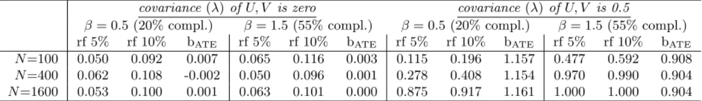
Table 1: Simulation results

covariance (λ) of U, V is zero covariance (λ) of U, V is 0.5

β = 0.5 (20% compl.) β = 1.5 (55% compl.) β = 0.5 (20% compl.) β = 1.5 (55% compl.) rf 5% rf 10% bATE rf 5% rf 10% bATE rf 5% rf 10% bATE rf 5% rf 10% bATE

N =100 0.050 0.092 0.007 0.065 0.116 0.003 0.115 0.196 1.157 0.477 0.592 0.908 N =400 0.062 0.108 -0.002 0.050 0.096 0.001 0.278 0.408 1.154 0.970 0.990 0.904 N =1600 0.053 0.100 0.001 0.063 0.101 0.000 0.875 0.917 1.161 1.000 1.000 0.904

Note: rf 5%, 10%: Rejection frequencies at the 5% and 10% significance level. bATE: Bias of the ATE.

Table 1 reports the rejection frequencies of the Wald test (with heteroskedasticity robust

covariance matrix) at the 5% and 10% significance levels (rf 5%, rf 10%) for 1000 simulations

and three sample sizes N . The bias of estimating the ATE on the entire population by the mean

difference in treated and non-treated outcomes is also provided (bATE). For λ = 0, the rejection

frequencies are close to the nominal sizes while estimation bias is small and decreasing in N . For

λ = 0.5 (violation of Assumption 3), the bias is substantial and does not vanish asymptotically.

The test gains power in the share of compliers and N . Our results suggest that testing is powerful

even in moderate samples if the complier population is not too small.

References

Angrist, J., G. Imbens, andD. Rubin (1996): “Identification of Causal Effects using Instru-mental Variables,” Journal of American Statistical Association, 91, 444–472 (with discussion). de Luna, X., and P. Johansson (2012): “Testing for Nonparametric Identification of Causal

Effects in the Presence of a Quasi-Instrument,” IZA Discussion Paper No. 6692.

Donald, S. G., Y.-C. Hsu, and R. P. Lieli (2011): “Testing the Unconfoundedness As-sumption via Inverse Probability Weighted Estimators of (L)ATT,” unpublished mansucript, University of Texas, Austin.

Pearl, J. (1995): “Causal Diagrams for Empirical Research,” Biometrika, 82, 669–688.

Rubin, D. B. (1974): “Estimating Causal Effects of Treatments in Randomized and Nonran-domized Studies,” Journal of Educational Psychology, 66, 688–701.