Time complexity of concurrent programs

HAL Id: hal-01229068

https://hal.inria.fr/hal-01229068

Submitted on 16 Nov 2015

HAL is a multi-disciplinary open access

archive for the deposit and dissemination of

sci-entific research documents, whether they are

pub-lished or not. The documents may come from

teaching and research institutions in France or

abroad, or from public or private research centers.

L’archive ouverte pluridisciplinaire HAL, est

destinée au dépôt et à la diffusion de documents

scientifiques de niveau recherche, publiés ou non,

émanant des établissements d’enseignement et de

recherche français ou étrangers, des laboratoires

publics ou privés.

Time complexity of concurrent programs

Elena Giachino, Einar Broch Johnsen, Cosimo Laneve, Ka I Pun

To cite this version:

Elena Giachino, Einar Broch Johnsen, Cosimo Laneve, Ka I Pun. Time complexity of concurrent

programs: a technique based on behavioural types. FACS 2015, Oct 2015, Niterói, Rio de Janeiro,

Brazil. �hal-01229068�

Time complexity of concurrent programs

⋆

– a technique based on behavioural types –

Elena Giachino1, Einar Broch Johnsen2, Cosimo Laneve1, and Ka I Pun2

1 _{Dept. of Computer Science and Engineering, University of Bologna – INRIA FOCUS}

2 _{Dept. of Informatics, University of Oslo}

Abstract. We study the problem of automatically computing the time complex-ity of concurrent object-oriented programs. To determine this complexcomplex-ity we use intermediate abstract descriptions that record relevant information for the time analysis (cost of statements, creations of objects, and concurrent opera-tions), called behavioural types. Then, we define a translation function that takes behavioural types and makes the parallelism explicit into so-called cost

equa-tions, which are fed to an automatic off-the-shelf solver for obtaining the time complexity.

1

Introduction

Computing the cost of a sequential algorithm has always been a primary question for every programmer, who learns the basic techniques in the first years of their computer science or engineering curriculum. This cost is defined in terms of the input values to the algorithm and over-approximates the number of the executed instructions. In turn, given an appropriate abstraction of the CPU speed of a runtime system, one can obtain the expected computation time of the algorithm.

The computational cost of algorithms is particularly relevant in mainstream archi-tectures, such as the cloud. In that context, a service is a concurrent program that must comply with a so-called service-level agreement (SLA) regulating the cost in time and assigning penalties for its infringement [3]. The service provider needs to make sure that the service is able to meet the SLA, for example in terms of the end-user response time, by deciding on a resource management policy and determining the appropriate number of virtual machine instances (or containers) and their parameter settings (e.g., their CPU speeds). To help service providers make correct decisions about the resource management before actually deploying the service, we need static analysis methods for resource-aware services [6]. In previous work by the authors, cloud deployments expressed in the formal modeling language ABS [8] have used a combination of cost analysis and simulations to analyse resource management [1], and a Hoare-style proof system to reason about end-user deadlines has been developed for sequential execu-tions [7]. In contrast, we are here interested in statically estimating the computation time of concurrent services deployed on the cloud with a given dynamic resource man-agement policy.

⋆_{Supported by the EU projects FP7-610582 Envisage: Engineering Virtualized Services}

Technically, this paper proposes a behavioural type system expressing the resource costs associated with computations and study how these types can be used to soundly calculate the time complexity of parallel programs deployed on the cloud. To succinctly formulate this problem, our work is developed for tml, a small formally defined con-current object-oriented language which uses asynchronous communications to trigger parallel activities. The language defines virtual machine instances in terms of dynam-ically created concurrent object groups with bounds on the number of cycles they can perform per time interval. As we are interested in the concurrent aspects of these com-putations, we abstract from sequential analysis in terms of a statement job(e), which defines the number of processing cycles required by the instruction – this is similar to the sleep(n) operation in Java.

The analysis of behavioural types is defined by translating them in a code that is adequate for an off-the-shelf solver – the CoFloCo solver [4]. As a consequence, we are able to determine the computational cost of algorithms in a parametric way with respect to their inputs.

Paper overview.The language is defined in Section 2 and we discuss restrictions that ease the development of our technique in Section 3. Section 4 presents the behavioural type system and Section 5 explains the analysis of computation time based on these behavioural types. In Section 6 we outline our correctness proof of the type system with respect to the cost equations. In Section 7 we discuss the relevant related work and in Section 8 we deliver concluding remarks.

2

The language tml

The syntax and the semantics of tml are defined in the following two subsections; the third subsection discusses a few examples.

Syntax. A tml program is a sequence of method definitions T m(T x){ F y ; s }, ranged

over by M, plus a main body { F z ; s′}with k. In tml we distinguish between

sim-ple types T which are either integers Int or classes Class (there is just one class in tml), and types F, which also include future types Fut<T >. These future types let asyn-chronous method invocations be typed (see below). The notation T x denotes any finite sequence of variable declarations T x. The elements of the sequence are separated by

commas. When we write T x ; we mean a sequence T1 x1 ; · · · ;Tn xn ;when the

sequence is not empty; we mean the possibly empty sequence otherwise.

The syntax of statements s, expressions with side-effects z and expressions e of tml is defined by the following grammar:

s::= x = z | if e { s } else { s } | job(e) | return e | s ; s

z::= e | e!m(e) | e.m(x) | e.get | new Class with e | new local Class

e::= this | se | nse

A statement s may be either one of the standard operations of an imperative language or the job statement job(e) that delays the continuation by e cycles of the machine executing it.

An expression z may change the state of the system. In particular, it may be an

execution. When the value computed by the invocation is needed, the caller performs a

non-blocking getoperation: if the value needed by a process is not available, then an awaiting process is scheduled and executed, i.e., await-get. Expressions z also include standard synchronous invocations e.m(e) and new local Class, which creates a new object. The intended meaning is to create the object in the same machine – called cog or concurrent object group – of the caller, thus sharing the processor of the caller: op-erations in the same virtual machine interleave their evaluation (even if in the following operational semantics the parallelism is not explicit). Alternatively, one can create an object on a different cog with new Class with e thus letting methods execute in paral-lel. In this case, e represents the capacity of the new cog, that is, the number of cycles the cog can perform per time interval. We assume the presence of a special identifier

this.capacitythat returns the capacity of the corresponding cog.

A pure expression e can be the reserved identifier this or an integer expression. Since the analysis in Section 5 cannot deal with generic integer expressions, we parse expressions in a careful way. In particular we split them into size expressions se, which are expressions in Presburger arithmetics (this is a decidable fragment of Peano arith-metics that only contains addition), and non-size expressions nse, which are the other type of expressions. The syntax of size and non-size expressions is the following:

nse::= k | x | nse ≤ nse | nse and nse | nse or nse

| nse + nse | nse − nse | nse × nse | nse/nse

se::= ve | ve ≤ ve | se and se | se or se

ve::= k | x | ve + ve | k × ve

k::= rational constants

In the paper, we assume that sequences of declarations T x and method declarations

M do not contain duplicate names. We also assume that return statements have no

continuation.

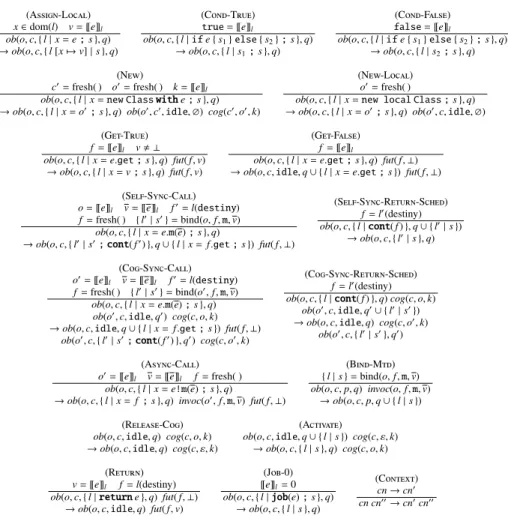
Semantics. The semantics of tml is defined by a transition system whose states are

configurations cnthat are defined by the following syntax.

cn::= ε | fut( f, val) | ob(o, c, p, q) | invoc(o, f, m, v) act::= o | ε

| cog(c, act, k) | cn cn val::= v | ⊥

p::= { l | s } | idle l::= [· · · , x 7→ v, · · · ]

q::= ∅ | { l | s } | q q v::= o | f | k

A configuration cn is a set of concurrent object groups (cogs), objects, invocation messages and futures, and the empty configuration is written as ε. The associative and commutative union operator on configurations is denoted by whitespace. A cog is given as a term cog(c, act, k) where c and k are respectively the identifier and the capacity of the cog, and act specifies the currently active object in the cog. An object is written as ob(o, c, p, q), where o is the identifier of the object, c the identifier of the cog the object belongs to, p an active process, and q a pool of suspended processes. A process is written as { l | s }, where l denotes local variable bindings and s a list of statements. An invocation message is a term invoc(o, f , m, v) consisting of the callee o, the future

f to which the result of the call is returned, the method name m, and the set of actual parameter values for the call. A future fut( f , val) contains an identifier f and a reply value val, where ⊥ indicates the reply value of the future has not been received.

(Assign-Local) x ∈dom(l) v = [[e]]l ob(o, c, { l | x = e ; s }, q) → ob(o, c, { l [x 7→ v] | s }, q) (Cond-True) true= [[e]]l ob(o, c, { l | if e { s1} else { s2} ; s }, q) → ob(o, c, { l | s1;s }, q) (Cond-False) false= [[e]]l ob(o, c, { l | if e { s1} else { s2} ; s }, q) → ob(o, c, { l | s2;s }, q) (New) c′ = fresh( ) o′ = fresh( ) k = [[e]]l ob(o, c, { l | x = new Class with e ; s }, q) → ob(o, c, { l | x = o′_{;s }, q) ob(o}′_,c′_{,idle, ∅) cog(c}′_,o′_,k)

(New-Local)

o′ = fresh( )

ob(o, c, { l | x = new local Class ; s }, q) → ob(o, c, { l | x = o′_{;s }, q) ob(o}′_{,c, idle, ∅)} (Get-True)

f = [[e]]l v , ⊥ ob(o, c, { l | x = e.get ; s }, q) fut( f, v)

→ ob(o, c, { l | x = v ; s }, q) fut( f, v)

(Get-False)

f = [[e]]l

ob(o, c, { l | x = e.get ; s }, q) fut( f, ⊥) → ob(o, c, idle, q ∪ { l | x = e.get ; s }) fut( f, ⊥) (Self-Sync-Call)

o = [[e]]l v = [[e]]l f′= l(destiny) f = fresh( ) { l′_{| s}′_{} = bind(o, f, m, v)} ob(o, c, { l | x = e.m(e) ; s }, q) → ob(o, c, { l′_{| s}′_{; cont( f}′ ) }, q ∪ { l | x = f.get ; s }) fut( f, ⊥) (Self-Sync-Return-Sched) f = l′_(destiny) ob(o, c, { l | cont( f ) }, q ∪ { l′_{| s })} → ob(o, c, { l′_{| s }, q)} (Cog-Sync-Call) o′

= [[e]]l v = [[e]]l f′= l(destiny) f = fresh( ) { l′_{| s}′

} = bind(o′_{,f, m, v)}

ob(o, c, { l | x = e.m(e) ; s }, q)

ob(o′_{,c, idle, q}′_{) cog(c, o, k)} → ob(o, c, idle, q ∪ { l | x = f.get ; s }) fut( f, ⊥)

ob(o′_{,c, { l}′_{| s}′_{; cont( f}′_{) }, q}′_{) cog(c, o}′_,k)

(Cog-Sync-Return-Sched)

f = l′_(destiny)

ob(o, c, { l | cont( f ) }, q) cog(c, o, k)

ob(o′_{,c, idle, q}′_{∪ { l}′_{| s}′_}) → ob(o, c, idle, q) cog(c, o′_,k)

ob(o′_{,c, { l}′_{| s}′_{}, q}′₎

(Async-Call)

o′

= [[e]]l v = [[e]]l f = fresh( ) ob(o, c, { l | x = e!m(e) ; s }, q)

→ ob(o, c, { l | x = f ; s }, q) invoc(o′_{,f, m, v) fut( f, ⊥)}

(Bind-Mtd) { l | s } = bind(o, f, m, v)

ob(o, c, p, q) invoc(o, f, m, v) → ob(o, c, p, q ∪ { l | s })

(Release-Cog)

ob(o, c, idle, q) cog(c, o, k) → ob(o, c, idle, q) cog(c, ε, k)

(Activate)

ob(o, c, idle, q ∪ { l | s }) cog(c, ε, k) → ob(o, c, { l | s }, q) cog(c, o, k)

(Return)

v = [[e]]l f = l(destiny) ob(o, c, { l | return e }, q) fut( f, ⊥)

→ ob(o, c, idle, q) fut( f, v)

(Job-0) [[e]]l= 0 ob(o, c, { l | job(e) ; s }, q) → ob(o, c, { l | s }, q) (Context) cn → cn′ cn cn′′_{→ cn}′_cn′′

Fig. 1. The transition relation of tml – part 1.

The following auxiliary function is used in the semantic rules for invocations. Let

T′m(T x){ F x′_{; s } be a method declaration. Then}

bind(o, f , m, v) = { [destiny 7→ f, x 7→ v, x′_{7→ ⊥] | s{}o_{/this} }}

The transition rules of tml are given in Figures 1 and 2. We discuss the most rel-evant ones: object creation, method invocation, and the job(e) operator. The creation of objects is handled by rules New and New-Local: the former creates a new object inside a new cog with a given capacity e, the latter creates an object in the local cog. Method invocations can be either synchronous or asynchronous. Rules Self-Sync-Call and Cog-Sync-Call specify synchronous invocations on objects belonging to the same cog of the caller. Asynchronous invocations can be performed on every object.

(Tick) strongstablet(cn) cn → Φ(cn, t) where Φ_{(cn, t) =}                                ob(o, c, {l′_|job(k′_{) ; s}, q) Φ(cn}′_,t) if cn = ob(o, c, {l | job(e) ; s}, q) cn′ and cog(c, o, k) ∈ cn′ and k′_{= [[e]]} l− k ∗ t

ob(o, c, idle, q) Φ(cn′_{,t) if cn = ob(o, c, idle, q) cn}′

cn otherwise.

Fig. 2. The transition relation of tml – part 2: the strongly stable case

In our model, the unique operation that consumes time is job(e). We notice that the reduction rules of Figure 1 are not defined for the job(e) statement, except the trivial case when the value of e is 0. This means that time does not advance while non-job statements are evaluated. When the configuration cn reaches a stable state, i.e., no other transition is possible apart from those evaluating the job(e) statements, then the time is advanced by the minimum value that is necessary to let at least one process start. In order to formalize this semantics, we define the notion of stability and the update

operationof a configuration cn (with respect to a time value t). Let [[e]]lreturn the value

of e when variables are bound to values stored in l.

Definition 1. Let t > 0. A configuration cn is t-stable, written stablet(cn), if any object

in cn is in one of the following forms:

1. ob(o, c, { l | job(e); s }, q) with cog(c, o, k) ∈ cn and [[e]]l/k ≥ t,

2. ob(o, c, idle, q) and

i. either q = ∅,

ii. or, for every p ∈ q, p = { l | x = e.get; s } with [[e]]l= f and fut( f, ⊥),

iii. or, cog(c, o′_{,k) ∈ cn where o , o}′_{, and o}′_{satisfies Definition 1.1.}

A configuration cn isstrongly t-stable, written strongstablet(cn), if it is t-stable and

there is an object ob(o, c, { l | job(e); s }, q) with cog(c, o, k) ∈ cn and [[e]]l/k = t.

Notice that t-stable (and, consequently, strongly t-stable) configurations cannot progress anymore because every object is stuck either on a job or on unresolved get statements. The update of cn with respect to a time value t, noted Φ(cn, t) is defined in Figure 2. Given these two notions, rule Tick defines the time progress.

The initial configuration of a program with main method { F x; s } with k is

ob(start, start, { [destiny 7→ fstart,x 7→ ⊥] | s }, ∅)

cog(start, start, k)

where start and start are special cog and object names, respectively, and fstartis a fresh

Examples. To begin with, we discuss the Fibonacci method. It is well known that the computational cost of its sequential recursive implementation is exponential. However, this is not the case for the parallel implementation. Consider

Int fib(Int n) {

if (n<=1) { return 1; }

else { Fut<Int> f; Class z; Int m1; Int m2;

job(1);

z = new Class with this.capacity ; f = this!fib(n-1); g = z!fib(n-2); m1 = f.get; m2 = g.get;

return m1 + m2;

} }

Here, the recursive invocation fib(n-1) is performed on the this object while the invocation fib(n-2) is performed on a new cog with the same capacity (i.e., the object referenced by z is created in a new cog set up with this.capacity), which means that it can be performed in parallel with the former one. It turns out that the cost of the following invocation is n.

Class z; Int m; Int x; x = 1;

z = new Class with x; m = z.fib(n);

Observe that, by changing the line x = 1; into x = 2; we obtain a cost of n/2. Our semantics does not exclude paradoxical behaviours of programs that perform infinite actions without consuming time (preventing rule Tick to apply), such as this one

Int foo() { Int m; m = this.foo(); return m; }

This kind of behaviours are well-known in the literature, (cf. Zeno behaviours) and they may be easily excluded from our analysis by constraining recursive invocations to be prefixed by a job(e)-statement, with a positive e. It is worth to observe that this condition is not sufficient to eliminate paradoxical behaviours. For instance the method below does not terminate and, when invoked with this.fake(2), where this is in a cog of capacity 2, has cost 1.

Int fake(Int n) { Int m; Class x;

x = new Class with 2*n; job(1); m = x.fake(2*n); return m; }

Imagine a parallel invocation of the following method Int one() { job(1); }

on an object residing in a cog of capacity 1. At each stability point the job(1) of the latter method will compete with the job(1) of the former one, which will win every time, since having a greater (and growing) capacity it will require always less time. So at

the first stability point we get job(1−1/2) (for the method one), then job(1−1/2−1/4) and so on, thus this sum will never reach 0.

In the examples above, the statement job(e) is a cost annotation that specifies how many processing cycles are needed by the subsequent statement in the code. We notice that this operation can also be used to program a timer which suspends the current execution for e units of time. For instance, let

Int wait(Int n) { job(n); return 0; } Then, invoking wait on an object with capacity 1

Class timer; Fut<Class> f; Class x; timer = new Class with 1;

f = timer!wait(5); x = f.get;

one gets the suspension of the current thread for 5 units of time.

3

Issues in computing the cost of tml programs

The computation time analysis of tml programs is demanding. To highlight the diffi-culties, we discuss a number of methods.

Int wrapper(Class x) { Fut<Int> f; Int z;

job(1) ; f = x!server(); z = f.get; return z;

}

Method wrapper performs an invocation on its argument x. In order to determine the cost of wrapper, we notice that, if x is in the same cog of the carrier, then its cost is (assume that the capacity of the carrier is 1): 1 + cost(server) because the two invocations are sequentialized. However, if the cogs of x and of the carrier are different, then we are not able to compute the cost because we have no clue about the state of the cog of x. Next consider the following definition of wrapper

Int wrapper_with_log(Class x) { Fut<Int> f; Fut<Int> g; Int z;

job(1) ; f = x!server(); g = x!print_log(); z = f.get; return z;

}

In this case the wrapper also asks the server to print its log and this invocation is not synchronized. We notice that the cost of wrapper_with_log is not anymore

1+cost(server) (assuming that x is in the same cog of the carrier) because print_log

might be executed before server. Therefore the cost of wrapper_with_log is 1 +

cost_{(server) + cost(print log).}

Finally, consider the following wrapper that also logs the information received from the server on a new cog without synchronising with it:

Int wrapper_with_external_log(Class x) { Fut<Int> f; Fut<Int> g; Int z; Class y;

job(1) ; f = x!server(); g = x!print_log(); z = f.get; y = new Class with 1;

f = y!external_log(z) ; return z;

}

What is the cost of wrapper_with_external_log? Well, the answer here is debat-able: one might discard the cost of y!external_log(z) because it is useless for the value returned by wrapper_with_external_log, or one might count it because one wants to count every computation that has been triggered by a method in its cost. In this paper we adhere to the second alternative; however, we think that a better solution should be to return different cost for a method: a strict cost, which spots the cost that is necessary for computing the returned value, and an overall cost, which is the one computed in this paper.

Anyway, by the foregoing discussion, as an initial step towards the time analysis of

tmlprograms, we simplify our analysis by imposing the following constraint:

– it is possible to invoke methods on objects either in the same cog of the caller or on

newly created cogs.

The above constraint means that, if the callee of an invocation is one of the arguments of a method then it must be in the same cog of the caller. It also means that, if an invocation is performed on a returned object then this object must be in the same cog of the carrier. We will enforce these constraints in the typing system of the following section – see rule T-Invoke.

4

A behavioural type system for tml

In order to analyse the computation time of tml programs we use abstract descriptions, called behavioural types, which are intermediate codes highlighting the features of tml programs that are relevant for the analysis in Section 5. These abstract descriptions support compositional reasoning and are associated to programs by means of a type system. The syntax of behavioural types is defined as follows:

t::= -- | se | c[se] basic value

x::= f | t extended value

a::= e | νc[se] | m(t) →t | ν f: m(t) →t | f

X

atom

b::= a⊲ Γ | a#b | (se){b} | b+b behavioural type

where c, c′, · · · range over cog names and f , f′, · · · range over future names. Basic valuestare either generic (non-size) expressions -- or size expressions se or the type

c[se] of an object of cog c with capacity se. The extended values add future names to basic values.

Atomsadefine creation of cogs (νc[se]), synchronous and asynchronous method

invocations (m(t) →tand ν f : m(t) →t, respectively), and synchronizations on

asyn-chronous invocations ( fX

). We observe that cog creations always carry a capacity, which has to be a size expression because our analysis in the next section cannot deal

with generic expressions. Behavioural typesb are sequences of atomsa#b

′

or con-ditionals, typically (se){b} + (¬se){b

′_}

orb+b

′

, according to whether the boolean guard is a size expression that depends on the arguments of a method or not. In order to type sequential composition in a precise way (see rule T-Seq), the leaves of behavioural types are labelled with environments, ranged over by Γ, Γ′_{, · · · . Environments are maps}

from method names m to terms (t) →t, from variables to extended valuesx, and from

future names to values that are eithertort

X

.

The abstract behaviour of methods is defined by method behavioural types of the form: m(tt,t){b}:tr, wherettis the type value of the receiver of the method,tare the

type value of the arguments,bis the abstract behaviour of the body, andtris the type

value of the returned object. The subtermtt,t of the method contract is called header;

tr is called returned type value. We assume that names in the header occur linearly.

Names in the header bind the names inband intr. The header and the returned type

value, written (tt,t) →tr, are called behavioural type signature. Names occurring inb

ortrmay be not bound by header. These free names correspond to new cog creations

and will be replaced by fresh cog names during the analysis. We useCto range over

method behavioural types.

The type system uses judgments of the following form: – Γ ⊢ e :xfor pure expressions e, Γ ⊢ f :tor Γ ⊢ f :t

X

for future names f , and Γ⊢ m(t) :tfor methods.

– Γ ⊢ z :x,

[

a⊲ Γ

′

_]

for expressions with side effects z, wherexis the value,a⊲ Γ

′

is the corresponding behavioural type, where Γ′is the environment Γ with possible

updatesof variables and future names.

– Γ ⊢ s :b, in this case the updated environments Γ

′_{are inside the behavioural type,}

in correspondence of every branch of its.

Since Γ is a function, we use the standard predicates x ∈ dom(Γ) or x < dom(Γ). Moreover, we define Γ[x 7→x](y) def = ( x if y = x Γ(y) otherwise

The multi-hole contexts C[ ] are defined by the following syntax:

C_{[ ] ::=} [ ] | a# C[ ] | C[ ] + C[ ] | (se){ C[ ] }

and, wheneverb= C[a1⊲ Γ1] · · · [an⊲ Γn], thenb[x 7→x] is defined as C[a1⊲ Γ1[x 7→ x]] · · · [an⊲ Γn[x 7→x]].

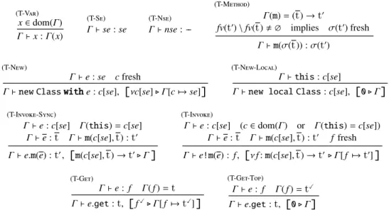
The typing rules for expressions are defined in Figure 3. These rules are not standard because (size) expressions containing method’s arguments are typed with the expres-sions themselves. This is crucial to the cost analysis in Section 5. In particular, cog

cre-ationis typed by rule T-New, with value c[se], where c is the fresh name associated with the new cog and se is the value associated with the declared capacity. The behavioural type for the cog creation is νc[se] ⊲ Γ[c 7→ se], where the newly created cog is added to Γ. In this way, it is possible to verify whether the receiver of a method invocation is within a locally created cog or not by testing whether the receiver belongs to dom(Γ) or not, respectively (cf. rule T-Invoke). Object creation (cf. rule T-New-Local) is typed as the cog creation, with the exception that the cog name and the capacity value are taken

(T-Var) x ∈dom(Γ) Γ⊢ x: Γ(x) (T-Se) Γ⊢ se: se (T-Nse) Γ⊢ nse: --(T-Method) Γ_{(m) = (}t) →t ′ fv(t ′_{) \ fv(} t) , ∅ implies σ(t ′_{) fresh} Γ⊢ m(σ(t)) : σ(t ′₎ (T-New) Γ⊢ e: se cfresh

Γ⊢ new Class with e: c[se],

[

νc[se] ⊲ Γ[c 7→ se]

]

(T-New-Local)

Γ⊢ this: c[se]

Γ⊢ new local Class: c[se],

[

0 ⊲ Γ

]

(T-Invoke-Sync)

Γ⊢ e: c[se] Γ_{(this) = c[se]} Γ⊢ e:t Γ⊢ m(c[se],t) :t ′ Γ⊢ e.m(e) :t ′_,

_[

_m(c[se], t) →t ′_{⊲ Γ}

_]

(T-Invoke)

Γ⊢ e: c[se] (c ∈ dom(Γ) or Γ_{(this) = c[se])}

Γ⊢ e:t Γ⊢ m(c[se],t) :t ′ _ffresh Γ⊢ e!m(e) : f ,

[

νf: m(c[se],t) →t ′_{⊲ Γ[ f 7→} t ′_]

_]

(T-Get) Γ⊢ e: f Γ_{( f ) =}t Γ⊢ e.get:t,

[

f X ⊲ Γ[ f 7→t X ]

]

(T-Get-Top) Γ⊢ e: f Γ_{( f ) =}t X Γ⊢ e.get:t,

[

0 ⊲ Γ

]

Fig. 3. Typing rules for expressions

from the local cog and the behavioural type is empty. Rule T-Invoke types method

invo-cations e!m(e) by using a fresh future name f that is associated to the method name, the cog name of the callee and the arguments. In the updated environment, f is associated with the returned value. Next we discuss the constraints in the premise of the rule. As we discussed in Section 2, asynchronous invocations are allowed on callees located in the current cog, Γ(this) = c[se], or on a newly created object which resides in a fresh cog, c ∈ dom(Γ). Rule T-Get defines the synchronization with a method invocation that corresponds to a future f . The expression is typed with the valuetof f in the

environ-ment and behavioural type fX

. Γ is then updated for recording that the synchronization has been already performed, thus any subsequent synchronization on the same value would not imply any waiting time (see that in rule T-Get-Top the behavioural type is 0). The synchronous method invocation in rule T-Invoke-Sync is directly typed with the return valuet

′_{of the method and with the corresponding behavioural type. The rule}

enforces that the cog of the callee coincides with the local one.

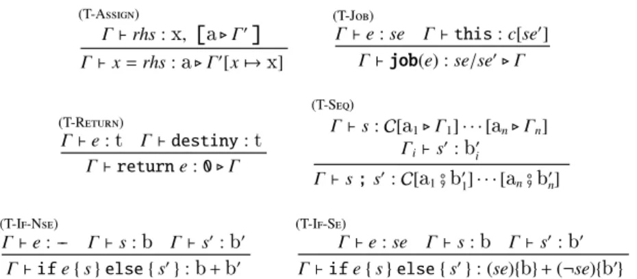
The typing rules for statements are presented in Figure 4. The behavioural type in rule T-Job expresses the time consumption for an object with capacity se′to perform se processing cycles: this time is given by se/se′, which we observe is in general a rational number. We will return to this point in Section 5.

The typing rules for method and class declarations are shown in Figure 5.

Examples The behavioural type of the fib method discussed in Section 2 is fib (c[x],n) {

(n ≤ 1){ 0 ⊲ ∅ } +

(T-Assign) Γ⊢ rhs:x,

[

a⊲ Γ ′

_]

Γ_{⊢ x = rhs :}a⊲ Γ ′_{[x 7→} x] (T-Job) Γ⊢ e: se Γ⊢ this: c[se′_] Γ⊢job(e) : se/se′_{⊲ Γ} (T-Return) Γ⊢ e:t Γ⊢ destiny:t Γ⊢ return e: 0 ⊲ Γ (T-Seq) Γ⊢ s: C[a1⊲ Γ1] · · · [an⊲ Γn] Γi⊢ s′:b ′ i Γ⊢ s ; s′_{: C[} a1#b ′ 1] · · · [an#b ′ n] (T-If-Nse) Γ⊢ e: -- Γ⊢ s:b Γ⊢ s ′_: b ′ Γ⊢ if e { s } else { s′_}: b+b ′ (T-If-Se) Γ⊢ e: se Γ⊢ s:b Γ⊢ s ′_: b ′ Γ⊢ if e { s } else { s′_{}: (se){} b} + (¬se){b ′_}

Fig. 4. Typing rules for statements

(T-Method) Γ(m) = (tt,t) →tr Γ[this 7→tt][destiny 7→tr][x 7→t] ⊢ s : C[a1⊲ Γ1] · · · [an⊲ Γn] Γ⊢ T m(T x) { s } : m(tt,t){ C[a1⊲ ∅] · · · [an⊲ ∅] } :tr (T-Class) Γ⊢ M:C Γ[this 7→ start[k]][x 7→t] ⊢ s : C[a1⊲ Γ1] · · · [an⊲ Γn] Γ⊢ M { T x ; s } with k :C,C[a1⊲ ∅] · · · [an⊲ ∅]

Fig. 5. Typing rules for declarations

(n ≥ 2){ 1/ x # d[x] # νf: fib (c[x],n -1)→ -- # νg: fib (d[x],n -2)→ -- # fX # gX #0 ⊲ ∅ } } :

--5

The time analysis

The behavioural types returned by the system defined in Section 4 are used to compute upper bounds of time complexity of a tml program. This computation is performed by an off-the-shelf solver – the CoFloCo solver [4] – and, in this section, we discuss the translation of a behavioural type program into a set of cost equations that are fed to the solver. These cost equations are terms

m_{(x) = exp [se]}

where m is a (cost) function symbol, exp is an expression that may contain (cost) func-tion symbol applicafunc-tions (we do not define the syntax of exp, which may be derived

by the following equations; the reader may refer to [4]), and se is a size expression whose variables are contained in x. Basically, our translation maps method types into cost equations, where (i) method invocations are translated into function applications, and (ii) cost expressions se occurring in the types are left unmodified. The difficulties of the translation is that the cost equations must account for the parallelism of processes in different cogs and for sequentiality of processes in the same cog. For example, in the following code:

x = new Class with c; y = new Class with d; f = x!m (); g = y!n (); u = g. get ; u = f. get ;

the invocations of m and n will run in parallel, therefore their cost will be max(t, t′_),

where t is the time of executing m on x and t′ _{is the time executing n on y. On the}

contrary, in the code

x = new local Class ; y = new local Class ; f = x!m (); g = y!n (); u = g. get ; u = f. get ;

the two invocations are queued for being executed on the same cog. Therefore the time needed for executing them will be t +t′_{, where t is time needed for executing m on x, and}

t′is the time needed for executing n on y. To abstract away the execution order of the invocations, the execution time of all unsynchronized methods from the same cog are taken into account when one of these methods is synchronized with a get-statement. To avoid calculating the execution time of the rest of the unsynchronized methods in the same cog more than necessary, their estimated cost are ignored when they are later synchronized.

In this example, when the method invocation y!n() is synchronized with g.get, the estimated time taken is t + t′, which is the sum of the execution time of the two unsynchronized invocations, including the time taken for executing m on x because both

xand y are residing in the same cog. Later when synchronizing the method invocation

x!m(), the cost is considered to be zero because this invocation has been taken into account earlier.

The translate function. The translation of behavioural types into cost equations is car-ried out by the function translate, defined below. This function parses atoms, be-havioural types or declarations of methods and classes. We will use the following aux-iliary function that removes cog names from (tuples of)tterms:

⌊ ⌋ = ⌊e⌋ = e ⌊c_{[e]⌋ = e} ⌊t1, . . . ,tn⌋ = ⌊t1⌋, . . . , ⌊tn⌋

We will also use translation environments, ranged over by Ψ , Ψ′, · · · , which map future

names to pairs (e, m(t)) that records the (over-approximation of the) time when the

method has been invoked and the invocation.

In the case of atoms, translate takes four inputs: a translation environment Ψ , the cog name of the carrier, an over-approximated cost e of an execution branch, and the atoma. In this case, translate returns an updated translation environment and the

cost. It is defined as follows. translate(Ψ, c, e,a) =                                                                      (Ψ, e + e′_{) when} a= e ′ (Ψ, e) whena= νc[e ′_] (Ψ, e + m(⌊t⌋)) whena= m(t) →t ′ (Ψ [ f 7→ (e, m(t))], e) whena= (ν f : m(t) →t ′₎ (Ψ \ F, e + e1))) whena= f X and Ψ_{( f ) = (e}f,mf(c[e′],tf)) let F = { g | Ψ (g) = (eg,mg(c[e′],tg)) } then and e1=P { mg(⌊t ′ g⌋) | (eg,mg(t ′ g)) ∈ Ψ (F) } (Ψ \ F, max(e, e1+ e2)) whena= f X and Ψ ( f ) = (ef,mf(c′[e′],tf)) and c , c ′ let F = { g | Ψ (g) = (eg,mg(c′[e′],tg)) } then e1=P { mg(⌊t ′ g⌋) | (eg,mg(t ′ g)) ∈ Ψ (F) } and e2= max{ eg|(eg,mg(t ′ g)) ∈ Ψ (F) } (Ψ, e) whena= f X and f < dom(Ψ )

The interesting case of translate is when the atom is fX

. There are three cases: 1. The synchronization is with a method whose callee is an object of the same cog.

In this case its cost must be added. However, it is not possible to know when the method will be actually scheduled. Therefore, we sum the costs of all the methods running on the same cog (worst case) – the set F in the formula – and we remove them from the translation environment.

2. The synchronization is with a method whose callee is an object on a different cog c′. In this case we use the cost that we stored in Ψ ( f ). Let Ψ ( f ) = (ef,mf(c′[e′],tf)),

then ef represents the time of the invocation. The cost of the invocation is therefore

ef+ mf(e′,⌊tf⌋). Since the invocation is in parallel with the thread of the cog c, the

overall cost will be max(e, ef + mf(e′,⌊tf⌋)). As in case 1, we consider the worst

scheduler choice on c′_{. Therefore, instead of taking e}

f + mf(e′,⌊tf⌋), we compute

the cost of all the methods running on c′_{– the set F in the formula – and we remove}

them from the translation environment.

3. The future does not belong to Ψ . That is the cost of the invocation which has been already computed. In this case, the value e does not change.

In the case of behavioural types, translate takes as input a translation environ-ment, the cog name of the carrier, an over-approximated cost of the current execution branch (e1)e2, where e1 indicates the conditions corresponding to the branch, and the

behavioural typea. translate(Ψ, c, (e1)e2,b) =                                          {(Ψ′_,(e

1)e′₂) } whenb=a⊲ Γ and translate(Ψ, c, e2,a) = (Ψ

′_,e′ 2) C whenb=a#b ′ _{and translate(Ψ, c, e} 2,a) = (Ψ ′_,e′ 2) and translate(Ψ′_,c,(e 1)e′2,b ′ ) = C C ∪ C′ _when b=b1+b2 and translate(Ψ, c, (e1)e2,b1) = C and translate(Ψ, c, (e1)e2,b2) = C ′ C whenb= (e){b ′_{} and translate(Ψ, c, (e} 1∧ e)e2,b ′ ) = C

The translation of the behavioural types of a method is given below. Let dom(Ψ ) = { f1,· · · , fn}. Then we define ΨX def= f1

X # · · · #fn X . translate(m(c[e],t){b}:t) =              m(e, e) = e′ 1+ e ′′ 1 [e1] . . . m(e, e) = e′ n+ e′′n [en] where translate(∅, c, 0,b) = { Ψi,(ei)e ′ i |1 ≤ i ≤ n }, and e = ⌊t⌋, and e′′ i = translate(Ψi,c, 0, ΨiX⊲ ∅) .

In addition, [ei] are the conditions for branching the possible execution paths of method

m(e, e), and e′

i + e

′′

i is the over-approximation of the cost for each path. In particular,

e′

i corresponds to the cost of the synchronized operations in each path (e.g., jobs and

gets), while e′′

i corresponds to the cost of the asynchronous method invocations

trig-gered by the method, but not synchronized within the method body.

Examples We show the translation of the behavioural type of fibonacci presented in

Section 4. Let b = (se){0 ⊲ ∅} + (¬se){b

′_}

, where se = (n ≤ 1) and b

′ _{= 1/e #}

νf: fib(c[e], n − 1) → -- # νg: fib(c′_{[e], n − 2) → -- # f}X

# gX

# 0 ⊲ ∅}. Let also Ψ= Ψ1∪Ψ2, where Ψ1 = [ f 7→ (1/e, fib(e, n−1))] and Ψ2 = [g 7→ (1/e, fib(e, n−2))].

The following equations summarize the translation of the behavioural type of the fibonacci method.

translate(∅, c, 0,b)

= translate(∅, c, 0, (se) { 0 ⊲ ∅ }) ∪ translate(∅, c, 0, (¬se) {b

′_})

= translate(∅, c, (se)0, { 0 ⊲ ∅ }) ∪ translate(∅, c, (¬se)0, { 1/e # . . . }) = { (se)0 } ∪ translate(∅, c, (¬se)(1/e), { ν f : fib(c[e], n − 1) → -- # . . . }) = { (se)0 } ∪ translate(Ψ1,c,(¬se)(1/e), { νg: fib(c′[e], n − 2) → -- # . . . })

= { (se)0 } ∪ translate(Ψ, c, (¬se)(1/e), { fX

#gX

# . . . })

= { (se)0 } ∪ translate(Ψ2,c,(¬se)(1/e + fib(e, n − 1)), { gX# . . . })

= { (se)0 } ∪ translate(∅, c, (¬se)(1/e + max(fib(e, n − 1), fib(e, n − 2))), { 0 ⊲ ∅ }) = { (se)0 } ∪ { (¬se)(1/e + max(fib(e, n − 1), fib(e, n − 2))) }

translate(∅, c, 0, 0) = (∅, 0) translate(∅, c, 0, 1/e) = (∅, 1/e)

translate(∅, c, 1/e, ν f : fib(c[e], n − 1) → -- ) = (Ψ1,1/e)

translate(Ψ1,c,1/e, νg: fib(c′[e], n − 2) → -- ) = (Ψ, 1/e)

translate(Ψ, c, 1/e, fX

) = (Ψ2,1/e + fib(e, n − 1))

translate(Ψ2,c,1/e + fib(e, n − 1), gX) = (∅, 1/e + max(fib(e, n − 1), fib(e, n − 2)))

translate(fib (c[e], n){b}: --) =          fib(e, n) = 0 [n ≤ 1]

Remark 1. Rational numbers are produced by the rule T-Job of our type system. In

particular behavioural types may manifest terms se/se′where se gives the processing

cycles defined by the job operation and se′specifies the number of processing cycles per unit of time the corresponding cog is able to handle. Unfortunately, our backend solver – CoFloCo – cannot handle rationals se/se′_{where se}′_{is a variable. This is the}

case, for instance, of our fibonacci example, where the cost of each iteration is 1/x, where x is a parameter. In order to analyse this example, we need to determine a priori the capacity to be a constant – say 2 –, obtaining the following input for the solver: eq(f(E,N),0,[],[-N>=1,2*E=1]).

eq(f(E,N),nat(E),[f(E,N-1)],[N>=2,2*E=1]). eq(f(E,N),nat(E),[f(E,N-2)],[N>=2,2*E=1]). Then the solver gives the following upper bound: nat(N-1)* (1/2).

It is worth to notice that fixing the fibonacci method is easy because the capacity does not change during the evaluation of the method. This is not always the case, as in the following alternative definition of fibonacci:

Int fib_alt ( Int n) {

if (n <=1) { return 1; }

else { Fut <Int > f; Class z; Int m1 ; Int m2; job (1);

z = new Class with ( this . capacity *2) ; f = this ! fib_alt (n -1); g = z! fib_alt (n -2); m1 = f. get ; m2 = g. get ;

return m1 + m2; } }

In this case, the recursive invocation z!fib alt(n-2) is performed on a cog with twice the capacity of the current one and CoFloCo is not able to handle it. It is worth to observe that this is a problem of the solver, which is otherwise very powerful for most of the examples. Our behavioural types carry enough information for dealing with more complex examples, so we will consider alternative solvers or combination of them for dealing with examples like fib alt.

6

Properties

In order to prove the correctness of our system, we need to show that (i) the behavioural type system is correct, and (ii) the computation time returned by the solver is an upper bound of the actual cost of the computation.

The correctness of the type system in Section 4 is demonstrated by means of a subject reduction theorem expressing that if a runtime configuration cn is well typed and

cn → cn′_{then cn}′_{is well-typed as well, and the computation time of cn is larger or equal}

to that of cn′_{. In order to formalize this theorem we extend the typing to configurations}

and we also use extended behavioural typeskwith the following syntax

k::= b | [b]

c

The type [b] c

f expresses the behaviour of an asynchronous method bound to the future f

and running in the cog c; the typekk k

′

expresses the parallel execution of methods inkand ink

′

.

We then define a relation Dtbetween runtime behavioural types that relates types.

The definition is algebraic, andkDtk

′

is intended to mean that the computational time ofkis at least that ofk

′_{+ t (or conversely the computational time of}

k

′_{is at most that}

ofk− t). This is actually the purpose of our theorems.

Theorem 1 (Subject Reduction). Let cn be a configuration of a tml program and letk

be its behavioural type. If cn is not strongly t-stable and cn → cn′_{then there exists}

k

′

typing cn′_{such that}

kD0k

′_{. If cn is strongly t-stable and cn → cn}′_{then there exists}

k

′

typing cn′_{such that}

kDtk

′_.

The proof of is a standard case analysis on the last reduction rule applied.

The second part of the proof requires an extension of the translate function to runtime behavioural types. We therefore define a cost of the equations Ekreturned by

translate(k) – noted cost(E

k) – by unfolding the equational definitions.

Theorem 2 (Correctness). IfkDtk

′_{, then cost(E}

k) ≥ cost(Ek

′) + t.

As a byproduct of Theorems 1 and 2, we obtain the correctness of our technique, mod-ulo the correctness of the solver.

7

Related work

In contrast to the static time analysis for sequential executions proposed in [7], the paper proposes an approach to analyse time complexity for concurrent programs. Instead of using a Hoare-style proof system to reason about end-user deadlines, we estimate the execution time of a concurrent program by deriving the time-consuming behaviour with a type-and-effect system.

Static time analysis approaches for concurrent programs can be divided into two main categories: those based on type-and-effect systems and those based on abstract interpretation – see references in [9]. Type-and-effect systems (i) collect constraints on type and resource variables and (ii) solve these constraints. The difference with respect to our approach is that we do not perform the analysis during the type inference. We use the type system for deriving behavioural types of methods and, in a second phase, we use them to run a (non compositional) analysis that returns cost upper bounds. This dichotomy allows us to be more precise, avoiding unification of variables that are per-formed during the type derivation. In addition, we notice that the techniques in the liter-ature are devised for programs where parallel modules of sequential code are running. The concurrency is not part of the language, but used for parallelising the execution.

Abstract interpretation techniques have been proposed addressing domains carrying quantitative information, such as resource consumption. One of the main advantages of abstract interpretation is the fact that many practically useful optimization techniques have been developed for it. Consequently, several well-developed automatic solvers for cost analysis already exist. These techniques either use finite domains or use expedients

(widening or narrowing functions) to guarantee the termination of the fix-point gener-ation. For this reason, solvers often return inaccurate answers when fed with systems that are finite but not statically bounded. For instance, an abstract interpretation tech-nique that is very close to our contribution is [2]. The analysis of this paper targets a language with the same concurrency model as ours, and the backend solver for our analysis, CoFloCo, is a slightly modified version of the solver used by [2]. However the two techniques differ profoundly in the resulting cost equations and in the way they are produced. Our technique computes the cost by means of a type system, therefore every method has an associated type, which is parametric with respect to the arguments. Then these types are translated into a bunch of cost equations that may be composed with those of other methods. So our approach supports a technique similar to separate

com-pilation, and is able to deal with systems that create statically an unbounded but finite number of nodes. On the contrary, the technique in [2] is not compositional because it takes the whole program and computes the parts that may run in parallel. Then the cost equations are generated accordingly. This has the advantage that their technique does not have any restriction on invocations on arguments of methods that are (currently) present in our one.

We finally observe that our behavioural types may play a relevant role in a cloud computing setting because they may be considered as abstract descriptions of a method suited for SLA compliance.

8

Conclusions

This article presents a technique for computing the time of concurrent object-oriented programs by using behavioural types. The programming language we have studied fea-tures an explicit cost annotation operation that define the number of machine cycles required before executing the continuation. The actual computation activities of the pro-gram are abstracted by job-statements, which are the unique operations that consume time. The computational cost is then measured by introducing the notion of (strong)

t-stability (cf. Definition 1), which represents the ticking of time and expresses that up to t time steps no control activities are possible. A Subject Reduction theorem (The-orem 1), then, relates this stability property to the derived types by stating that the consumption of t time steps by job statements is properly reflected in the type system. Finally, Theorem 2 states that the solution of the cost equations obtained by translation of the types provides an upper bound of the execution times provided by the type system and thus, by Theorem 1, of the actual computational cost.

Our behavioural types are translated into so-called cost equations that are fed to a solver that is already available in the literature – the CoFloCo solver [4]. As discussed in Remark 1, CoFloCo cannot handle rational numbers with variables at the denom-inator. In our system, this happens very often. In fact, the number pc of processing cycles needed for the computation of a job(pc) is divided by the speed s of the machine running it. This gives the cost in terms of time of the job(pc) statement. When the ca-pacity is not a constant, but depends on the value of some parameter and changes over time, then we get the untreatable rational expression. It is worth to observe that this is a problem of the solver (otherwise very powerful for most of the examples), while

our behavioural types carry enough information for computing the cost also in these cases. We plan to consider alternative solvers or a combination of them for dealing with complex examples.

Our current technique does not address the full language. In particular we are still not able to compute costs of methods that contain invocations to arguments which do not live in the same machine (which is formalized by the notion of cog in our language). In fact, in this case it is not possible to estimate the cost without any indication of the state of the remote machine. A possible solution to this issue is to deliver costs of methods that are parametric with respect to the state of remote machines passed as argument. We will investigate this solution in future work.

In this paper, the cost of a method also includes the cost of the asynchronous invo-cations in its body that have not been synchronized. A more refined analysis, combined with the resource analysis of [5], might consider the cost of each machine, instead of the overall cost. That is, one should count the cost of a method per machine rather than in a cumulative way. While these values are identical when the invocations are always synchronized, this is not the case for unsynchronized invocation and a disaggregated analysis might return better estimations of virtual machine usage.

References

1. E. Albert, F. S. de Boer, R. H¨ahnle, E. B. Johnsen, R. Schlatte, S. L. Tapia Tarifa, and P. Y. H.

Wong. Formal modeling of resource management for cloud architectures: An industrial

case study using Real-Time ABS. Journal of Service-Oriented Computing and Applications, 8(4):323–339, 2014.

2. E. Albert, J. C. Fern´andez, E. B. Johnsen, and G. Rom´an-D´ıez. Parallel cost analysis of distributed systems. In Proceedings of SAS 2015, volume 9291 of Lecture Notes in Computer

Science. Springer, 2015. To appear.

3. R. Buyya, C. S. Yeo, S. Venugopal, J. Broberg, and I. Brandic. Cloud computing and emerging IT platforms: Vision, hype, and reality for delivering computing as the 5th utility. Future

Generation Comp. Sys., 25(6):599–616, 2009.

4. A. Flores Montoya and R. H¨ahnle. Resource analysis of complex programs with cost equa-tions. In Proceedings of 12th Asian Symposium on Programming Languages and Systems, volume 8858 of Lecture Notes in Computer Science, pages 275–295. Springer, 2014. 5. A. Garcia, C. Laneve, and M. Lienhardt. Static analysis of cloud elasticity. In Proceedings of

PPDP 2015, 2015.

6. R. H¨ahnle and E. B. Johnsen. Resource-aware applications for the cloud. IEEE Computer, 48(6):72–75, 2015.

7. E. B. Johnsen, K. I. Pun, M. Steffen, S. L. Tapia Tarifa, and I. C. Yu. Meeting deadlines, elastically. In From Action Systems to Distributed Systems: the Refinement Approach. CRC Press, 2015. To Appear.

8. E. B. Johnsen, R. Schlatte, and S. L. Tapia Tarifa. Integrating deployment architectures and resource consumption in timed object-oriented models. Journal of Logical and Algebraic

Methods in Programming, 84(1):67–91, 2015.

9. P. W. Trinder, M. I. Cole, K. Hammond, H. Loidl, and G. Michaelson. Resource analyses for parallel and distributed coordination. Concurrency and Computation: Practice and