HAL Id: hal-01307716
https://hal.sorbonne-universite.fr/hal-01307716
Submitted on 26 Apr 2016
HAL is a multi-disciplinary open access
archive for the deposit and dissemination of
sci-entific research documents, whether they are
pub-lished or not. The documents may come from
teaching and research institutions in France or
abroad, or from public or private research centers.
L’archive ouverte pluridisciplinaire HAL, est
destinée au dépôt et à la diffusion de documents
scientifiques de niveau recherche, publiés ou non,
émanant des établissements d’enseignement et de
recherche français ou étrangers, des laboratoires
publics ou privés.
Sea during summer: contrasting river inputs, ecosystem
metabolism and air–sea CO2 fluxes
A Forest, P Coupel, B Else, S Nahavandian, B Lansard, Patrick Raimbault, T
Papakyriakou, Y Gratton, L Fortier, J.-É Tremblay, et al.
To cite this version:
A Forest, P Coupel, B Else, S Nahavandian, B Lansard, et al.. Synoptic evaluation of carbon cycling
in the Beaufort Sea during summer: contrasting river inputs, ecosystem metabolism and air–sea CO2
fluxes. Biogeosciences, European Geosciences Union, 2014, 11 (10), pp.2827-2856.
�10.5194/bg-11-2827-2014�. �hal-01307716�
www.biogeosciences.net/11/2827/2014/ doi:10.5194/bg-11-2827-2014
© Author(s) 2014. CC Attribution 3.0 License.
Synoptic evaluation of carbon cycling in the Beaufort Sea during
summer: contrasting river inputs, ecosystem metabolism and
air–sea CO
2
fluxes
A. Forest1,*, P. Coupel1, B. Else2, S. Nahavandian3, B. Lansard4, P. Raimbault5, T. Papakyriakou2, Y. Gratton3,
L. Fortier1, J.-É. Tremblay1, and M. Babin1,6
1Takuvik Joint International Laboratory, Université Laval (Canada) – CNRS (France), Département de Biologie and Québec-Océan, Université Laval, Québec, G1V 0A6, Canada
2Centre for Earth Observation Science, University of Manitoba, Winnipeg, R3T 2N2, Canada
3Institut National de la Recherche Scientifique – Eau Terre Environnement, Québec, G1K 9A9, Canada
4Laboratoire des Sciences du Climat et de l’Environnement, IPSL-CEA-CNRS-Université de Versailles Saint-Quentin, 91198, Gif-sur-Yvette, France
5Aix-Marseille Univ., Mediterranean Institute of Oceanography (MIO), UMR7294, CNRS/INSU, UMR235, IRD, 13288, Marseille, CEDEX 09, Université du Sud Toulon-Var (MIO), 83957, La Garde CEDEX, France
6Laboratoire d’Océanographie de Villefranche, Université Pierre et Marie Curie (adjunct professor), 06238 Villefranche-sur-Mer Cedex, France
*now at: Golder Associates Ltd. 200-1170 boul Lebourgneuf, Québec, G2K 2E3, Canada
Correspondence to: A. Forest (alexandre_forest@golder.com)
Received: 5 August 2013 – Published in Biogeosciences Discuss.: 7 October 2013 Revised: 17 March 2014 – Accepted: 3 April 2014 – Published: 27 May 2014
Abstract. The accelerated decline in Arctic sea ice and
an ongoing trend toward more energetic atmospheric and oceanic forcings are modifying carbon cycling in the Arctic Ocean. A critical issue is to understand how net community production (NCP; the balance between gross primary pro-duction and community respiration) responds to changes and modulates air–sea CO2 fluxes. Using data collected as part of the ArcticNet–Malina 2009 expedition in the southeastern Beaufort Sea (Arctic Ocean), we synthesize information on sea ice, wind, river, water column properties, metabolism of the planktonic food web, organic carbon fluxes and pools, as well as air–sea CO2exchange, with the aim of documenting the ecosystem response to environmental changes. Data were analyzed to develop a non-steady-state carbon budget and an assessment of NCP against air–sea CO2 fluxes. During the field campaign, the mean wind field was a mild upwelling-favorable wind (∼ 5 km h−1) from the NE. A decaying ice cover (< 80 % concentration) was observed beyond the shelf, the latter being fully exposed to the atmosphere. We detected some areas where the surface mixed layer was net autotrophic owing to high rates of primary
produc-tion (PP), but the ecosystem was overall net heterotrophic. The region acted nonetheless as a sink for atmospheric CO2, with an uptake rate of −2.0 ± 3.3 mmol C m−2d−1 (mean ± standard deviation associated with spatial variabil-ity). We attribute this discrepancy to (1) elevated PP rates (> 600 mg C m−2d−1) over the shelf prior to our survey, (2) freshwater dilution by river runoff and ice melt, and (3) the presence of cold surface waters offshore. Only the Mackenzie River delta and localized shelf areas directly af-fected by upwelling were identified as substantial sources of CO2 to the atmosphere (> 10 mmol C m−2d−1). Daily PP rates were generally < 100 mg C m−2d−1 and cumu-lated to a total PP of ∼ 437.6 × 10³t C for the region over a 35-day period. This amount was about twice the or-ganic carbon delivery by river inputs (∼ 241.2 × 10³t C). Subsurface PP represented 37.4 % of total PP for the whole area and as much as ∼ 72.0 % seaward of the shelf break. In the upper 100 m, bacteria dominated (54 %) to-tal community respiration (∼ 250 mg C m−2d−1), whereas protozoans, metazoans, and benthos, contributed to 24, 10, and 12 %, respectively. The range of production-to-biomass
ratios of bacteria was wide (1–27 % d−1), while we esti-mated a narrower range for protozoans (6–11 % d−1) and metazoans (1–3 % d−1). Over the shelf, benthic biomass was twofold (∼ 5.9 g C m−2) the biomass of pelagic heterotrophs (∼ 2.4 g C m−2), in accord with high vertical carbon fluxes on the shelf (956 ± 129 mg C m−2d−1). Threshold PP (PP at which NCP becomes positive) in the surface layer oscillated from 20 to 152 mg C m−2d−1, with a pattern from low-to-high values as the distance from the Mackenzie River de-creased. We conclude that (1) climate change is exacerbating the already extreme biological gradient across the Beaufort shelf–basin system; (2) the Mackenzie Shelf acts as a weak sink for atmospheric CO2, suggesting that PP might exceed the respiration of terrigenous and marine organic matter in the surface layer; and (3) shelf break upwelling can transfer CO2to the atmosphere, but CO2outgassing can be attenuated if nutrients brought also by upwelling support diatom pro-duction. Our study underscores that cross-shelf exchange of waters, nutrients and particles is a key mechanism that needs to be properly monitored as the Arctic transits to a new state.
1 Introduction
As the seasonal ice zone (SIZ) expands with the ongoing re-treat in summer ice (Parkinson and Comiso, 2013), increased transport of water, solutes and particles is expected across the Arctic shelf break (Carmack and Chapman, 2003; For-est et al., 2007; Anderson et al., 2010). This is because sea ice and newly opened waters are both exposed to a more dynamic atmospheric forcing, which is a collateral effect of the amplified warming taking place at high northern latitudes (Francis and Vavrus, 2012). The synergy between a fractured, more mobile, sea ice cover and the development of large ar-eas devoid of sea ice creates the ideal pre-conditioning for increased cross-shelf exchange (e.g., O’Brien et al., 2011; Janout et al., 2013). The trend in atmospheric circulation over the Arctic since the late 1990s is an acceleration of the anticyclonic (clockwise) regime (Ogi and Rigor, 2013), recently exacerbated (since ∼ 2006–2007) by a marked in-tensification of the Beaufort Sea High (a prominent feature of high sea-level pressure) in early summer, which now fre-quently extends from northern North America to over Green-land (OverGreen-land et al., 2012; Moore, 2012). This intensifi-cation has translated into an increase in downward Ekman pumping in the Beaufort Gyre and stronger geostrophic cur-rents on its periphery (McPhee, 2013). Although the cyclonic (anticlockwise) regime is apparently in a declining trend in the Arctic during summer (Moore, 2012), coastal storminess is increasing (Vermaire et al., 2013) and the late summer sea-son is affected by a significant rise in the strength and size of cyclones (Simmonds and Keay, 2009). This trend in late summer storm activity apparently culminated in 2012 with the development of the so-called great Arctic cyclone
(Sim-monds and Rudeva, 2012; Zhang et al., 2013). As a result, stronger winds induced by both intensified high-pressure sys-tems and large-scale storms increase the potential for mo-mentum transfer and facilitate cross-shelf exchange during and around the period of minimum sea ice.
A prime consequence of increased lateral cross-shelf ex-change for ecosystem function and biogeochemical cycling in the Arctic is the upwelling of nutrient-rich and CO2 -rich (acidic) halocline waters (> 100 m) along the continental slope and over shallow shelves. On the one hand, upwelled nutrients sustain high primary production and associated ver-tical carbon export, thus resulting in the uptake of CO2by the surface biota and its subsequent storage at depth through the biological pump (e.g., Anderson et al., 2010; Tremblay et al., 2011). This process is, however, tightly linked to the structure of the pelagic food web, which dictates the pathways of bio-genic carbon flow in the water column (Forest et al., 2011). For example, a large biomass of microbial and/or metazoan heterotrophs in the surface layer could possibly negate the potential for CO2uptake if respiration exceeds primary pro-duction (e.g., Ortega-Retuerta et al., 2012). But if the respi-ration occurs below the mixed layer instead, such as when animals migrate to depth during the day or at the end of sum-mer, heterotrophic respiration might actually contribute to CO2storage in deeper waters (e.g., Darnis and Fortier, 2012; Kobari et al., 2013). On the other hand, upwelling brings up-ward acidic waters supersaturated in CO2with respect to the atmosphere (up to > 600 ppm), promoting CO2 outgassing and possibly impairing pelagic and benthic organisms sen-sitive to low pH (Yamamoto-Kawai et al., 2009; Mathis et al., 2012). These phenomena can be particularly strong in the Pacific sector of the Arctic Ocean where a water layer of Pacific origin containing ca. twice as much CO2as the deep Atlantic water mass lies at intermediate depths (see Lansard et al. 2012 for details).
Analyzing the interplay between hydrodynamics and ecosystem metabolism is a critical task if the implications of increased cross-shelf exchange for ocean acidification and CO2 sink-source balance are to be understood. Despite be-ing utterly needed, such analysis is challengbe-ing to realize, as a synoptic view of physical forcings, geochemical set-ting, and planktonic food web structure is logistically dif-ficult to obtain – especially for the Arctic marine environ-ment. Such evaluation is also complexified by the multiple timescales affecting the environmental and biological factors that govern carbon flux dynamics. Ecosystem metabolic bal-ance can be simplified as the net result of carbon fixation by autotrophic organisms minus that used by the whole biologi-cal community for respiration, which encompasses numerous processes in between (e.g., trophic transfer, reproduction, so-matic maintenance, motility). However, studies on ecosystem metabolism rarely go beyond the quantification of organic carbon production vs. remineralization, so the phenology of production vs. respiration, the food web components at play,
and the implications for air–sea CO2exchange often remain unexplored.
Here we synthesize information on atmospheric and hydrographic forcings, biogeochemical context, plankton metabolism, and air–sea CO2fluxes, as measured during the ArcticNet–Malina campaign that took place in July–August 2009 across the Mackenzie Shelf region (southeastern Beau-fort Sea, Arctic Ocean). This spatial-temporal window was particularly relevant to investigate the potential effects of changing atmospheric and sea ice patterns on the Arctic ma-rine ecosystem. Over that period, the Beaufort Sea was influ-enced by a shift from a high-pressure system fostering clear sky and strong northerly winds to a more cyclonic regime that promoted clouds and ice melt across the area (NSIDC, 2009). Our objective is to evaluate quantitatively the differ-ent fluxes and reservoirs of carbon across the shelf–basin in-terface to identify key indices of ecosystem response to cli-mate change. Hence, we pose three questions that will sup-port concluding on the potential interactions and feedbacks between ecological and biogeochemical processes with re-spect to carbon fluxes in the future Arctic Ocean: (1) to what extent was net ecosystem metabolism coupled with sea-to-air CO2fluxes? (2) What were the roles of cross-shelf exchange, river inputs and sea ice in driving carbon fluxes? (3) How did the planktonic food web respond and feed back to organic and inorganic carbon cycling?
2 Material and methods
2.1 Study area and sampling strategy
The Mackenzie Shelf in the southeastern Beaufort Sea is a narrow rectangular shelf (120 km width × 530 km length) bordered by the Alaskan Beaufort Shelf to the west, the Amundsen Gulf to the east, and by the Canada Basin to the north (Fig. 1). Galley et al. (2013) reviewed the atmo-spheric and sea ice conditions of the southern Beaufort Sea from 1996 to 2010. Over that period, ocean currents and sea ice circulation patterns were closely coupled, showing an anomalous anti-cyclonic pattern associated with an ac-centuated Beaufort Sea High when compared with the mean over 1981–2010 (Overland, 2009). The Beaufort Sea High was particularly strong in 2007, when Arctic sea ice ex-tent dramatically declined to 4.1 × 10⁶km2. Although less developed, a similar atmospheric pattern prevailed in sum-mer 2008 and for most of sumsum-mer 2009 (i.e., until August; NSIDC, 2009). Sea ice in the southern Beaufort Sea typically reaches a maximum thickness of ∼ 2–3 m in March–April and is usually melted by mid-September (Barber and Hane-siak, 2004). In April 2009, Haas et al. (2010) surveyed sea ice thicknesses in the region and found a wide range of condi-tions, from a multi-year sea ice cover of 2.3–3.3 m advected south by the anti-cyclonic motion of the Beaufort Gyre, to
a thin first-year ice of 1.1 m northwest of the Mackenzie Canyon.
Despite being the fourth largest river input in terms of freshwater discharge (330 km3yr−1), the Mackenzie River ranks first for sediment load among Arctic rivers, with an annual mean of 124 × 106t yr−1 (Gordeev, 2006). In 2009, the water discharge from the Mackenzie was above the mean of 1998–2008 from May to July (∼ 20.5 vs.
∼17.4 × 10³m3s−1) as well as during September–October (∼ 12.8 vs. ∼ 10.5 × 10³m3s−1), but was near the average in August (Forest et al., 2013). Typically in summer, ice melt and river runoff generate a stratified surface layer in the top 5–10 m of the water column (Carmack and Macdonald, 2002). Water masses in the region come from various sources and comprise sea ice meltwater, the Mackenzie River, the po-lar mixed layer (above ∼ 50 m), summer and winter water of Pacific origin (∼ 50–200 m), Atlantic Water (∼ 200–800 m), and Canada Basin deep water (> 800 m depth) (Lansard et al., 2012). Ocean circulation is complex and driven by wind and sea ice dynamics. Northwesterly winds retain sur-face waters and the Mackenzie River plume inshore (down-welling conditions), whereas easterlies push them seaward (upwelling conditions) (Macdonald and Yu, 2006). The re-cent wind-driven acceleration of the Beaufort Gyre (strength-ening of the Beaufort Sea High) has promoted the upwelling regime. Accordingly, a progressive switch from eastward to northwestward routing of surface waters has been observed since 2002 (Fichot et al., 2013).
Primary production (PP) in the Beaufort Sea is usu-ally known as being low when compared with other Arctic shelves, with an annual range from 30 to 70 g C m−2yr−1 (Sakshaug, 2004; Carmack et al., 2004). With the ongoing transformation of the atmosphere-ice regime in the Beaufort Sea, the vertical transport of nutrient-rich intermediate wa-ters to the surface through wind-driven upwelling appears to be able to increase PP on the shelf (Tremblay et al., 2011) and at its periphery (Forest et al., 2011). The strength of the spring bloom is closely related to the renewal of nitrate in the upper water column during winter (Tremblay et al., 2008). Then, a subsurface chlorophyll maximum (SCM) rapidly de-velops and progressively lowers the nitracline over summer (Martin et al., 2010). While large-sized diatom cells domi-nate the spring bloom, the SCM harbors a more diverse phy-toplankton community, numerically dominated by small flag-ellates. Planktonic and benthic food webs in the Macken-zie Shelf region are fueled by both allochthonous and au-tochthonous carbon sources (Parsons et al., 1989; Morata et al., 2008; Connelly et al., 2012). But the exact contribution of riverine material to overall ecosystem metabolism remains difficult to quantify, especially as stable isotopes and ele-mental ratios might provide a distorted view on food web linkages in the Beaufort Sea – i.e., biased toward terrige-nous inputs while PP is the primary organic carbon source (Sallon et al., 2011; Pineault et al., 2013). Nevertheless, it is impossible to dismiss the large organic matter flux from the
North America Arctic Ocean
141°W
138°W
135°W
132°W
129°W
126°W
Depth (m)
50
100
250
500
750
1000
25
Mackenzie River Mackenzie Delta72°N
71°N
70°N
69°N
Tuktoyaktuk Peninsula Cape Bathurst Amundsen Gulf Mackenzie Shelf Canada Basin Kugmallit Valley Mackenzie Canyon Anderson RiverSampling stations
Liverpool Bay Amundsen Gulf MouthSoutheast Beaufort Sea
Line 100 Line 200 Line 400 Line 500 St. 345 Line 300 Line 600 Line 700 ArcticNet stations Herschel Island
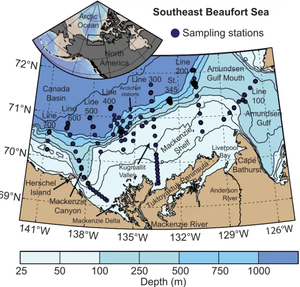
Figure 1. Map of the Mackenzie Shelf region (Beaufort Sea, Arctic Ocean) with position of sampling stations visited in July–August 2009
as part of the ArcticNet–Malina campaign. The ArcticNet sampling stations were located within the exploration license area EL446, whereas transects 100–700 and station 345 correspond to the Malina sampling grid. On each Malina transect, station numbers are listed in descending order from south to north (e.g., stations 170 to 110 from south to north on line 100). In this study, we used the following geographical limits when discussing the spatial variability: (i) the boundary between the shelf and the slope/basin is delineated by the 100 m isobath; and (ii) the western, central and eastern regions correspond to the areas delimited by 136–141◦W, 131–136◦W and 126–131◦W, respectively.
Mackenzie River. Previous studies comparing heterotrophic carbon demand versus local PP in the region typically pro-posed that riverine organic carbon input is the major factor explaining the imbalance between the two (e.g., Garneau et al., 2008; Ortega-Retuerta et al., 2012). While this might be appropriate for microbial communities, metazooplankton ac-tivity (dominated by copepods) is rather linked to pulses in fresh food supply during spring–summer (e.g., Forest et al., 2011, 2012). Similarly, carbon turnover by benthic organisms is largely related to the distribution of phyto-detritus in sur-face sediments (Renaud et al., 2007).
Here we used data from the ArcticNet and Malina oceano-graphic expeditions that successively investigated the south-eastern Beaufort Sea in July–August 2009 from the Canadian
research icebreaker CCGS Amundsen. The ArcticNet sam-pling stations were located within a small, enclosed area at the shelf break; whereas the Malina sampling grid was pri-marily composed of 7 shelf–basin transects (Fig. 1). Two of the Malina transects extended to very shallow waters (∼ 3 m depth) where sampling was conducted using a zodiac or a barge (see Doxaran et al., 2012). The ensemble of sampling stations conducted in July–August 2009 constitutes one of the most comprehensive spatial coverage of the Mackenzie Shelf region, within which a wide range of hydrographic, cryospheric and biogeochemical conditions were thoroughly sampled over a ∼ 1-month period.
Mixed-layer depth Air--sea CO2 exchange Bacteria Protozooplankton Metazooplankton Phytoplankton Respiration Respiration Respiration Respiration Production Production Production Production Excretion &
egestion Excretion &egestion
Excretion & egestion Excretion & egestion Biomass Biomass Biomass Biomass POC DOC Benthos Respiration Production Biomass Excretion & egestion Vertical fluxes River inputs Winds Ice concentration Remote sensing of primary production Nutrients T° and S Measured Data/model calculation Estimated
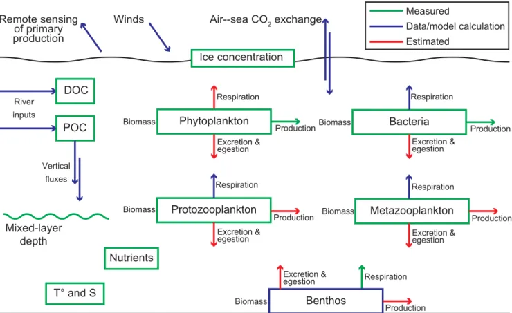
Figure 2. Diagram showing which variables have been directly measured on the field during ArcticNet–Malina, versus which ones have
been calculated using a combination of in situ data and statistical models, or rather estimated using knowledge from the literature or deduced from previous regional studies. This schematic aims at facilitating the reading of the methodological Sects. 2.2–2.6. The biophysical context at a regional scale prior and during the field campaign was documented using sea ice, wind and ocean color PP estimates gathered from different sources. For a detailed description of equations linking metabolic pathways of the planktonic and benthic compartments, please see Appendix B in Forest et al. (2011).
This study represents an effort to synthesize a wide range of observations made during the ArcticNet–Malina campaign in the context of previous work in the region and com-prises diverse data sets acquired through distinct approaches. Hence, to facilitate the reading of the following methodolog-ical sections, we provide a diagram (Fig. 2) showing which variables have been directly measured in the field, versus which ones have been calculated using a combination of in situ data and empirical/statistical models, or rather estimated using knowledge from the literature or deduced from pre-vious regional studies. Standard equations linking metabolic pathways of planktonic and benthic compartments were used (Forest et al., 2011). These equations bind ingestion (I ) to respiration (Re), egestion/excretion (e), secondary produc-tion (Ps), assimilation efficiency (AE), gross growth effi-ciency (GGE, for metazoans), or bacterial growth effieffi-ciency
(BGE, for bacteria).
I = Ps+Re+e (1) GGE = Ps/I (2) AE = (Ps+Re)/I (3) Re=I · (AE − GGE) (4) e = I · (1 − AE) (5) BGE = Ps/(Ps+Re) (6)
2.2 Sea ice conditions, wind reanalysis and ocean color
remote sensing
Daily averaged sea ice concentrations (% of cover) were ob-tained from the Ifremer-CERSAT team (http://cersat.ifremer. fr/) as initially acquired from the Special Sensor Microwave Imager (SSM/I) located onboard the orbiting sensor of the Defense Meteorological Satellite Program (DMSP). The CERSAT team processes ice maps at 12.5 km resolution using the daily brightness temperature maps from the Na-tional Snow and Ice Data Center (NSIDC; Maslanik and Stroeve, 1999) combined with the Artist Sea Ice algorithm of
Kaleschke et al. (2001). Sea ice concentrations for the study area were averaged over two 35-day periods (14 June–19 July and 20 July–24 August) to produce gridded composites of sea ice conditions in summer 2009.
Daily mean wind velocity and direction (meridional and zonal wind at 10 m) were obtained from the National Centers for Environmental Prediction (NCEP) North American Re-gional Reanalysis (NARR) (http://www.esrl.noaa.gov/psd/ data/gridded/data.narr.html). The NARR data are obtained from the high-resolution NCEP Eta Model (32 km, 45 lay-ers) together with the Regional Data Assimilation System (RDAS) and converted to a Northern Lambert Conformal Conic grid. Wind composites for the same periods as sea ice averages were computed.
Ocean color images from the Moderate Resolution Imag-ing Spectroradiometer (MODIS-Aqua; Level-3 daily Rrs at 412, 443, 488, 531, 555 and 667 nm) were downloaded from the NASA Goddard Earth Sciences Data and Informa-tion Services Center (http://oceancolor.gsfc.nasa.gov). For each image, PP rates were calculated using the processing chain and the photosynthesis-irradiance model of Bélanger et al. (2013). This procedure makes use of the state-of-the-art development in ocean color remote sensing and combines sea ice and cloud properties in order to model the incident spec-tral solar irradiance below the sea surface. It also accounts for absorption by colored dissolved organic matter (CDOM) and non-algal particles, which are known to increase artificially the ratio of chlorophyll (chl) a concentration to the diffuse attenuation coefficient of photosynthetically usable radiation. As this problem still remains a major issue in the coastal Arc-tic Ocean where river inputs are important (Ben Mustapha et al., 2012), we set a maximum chl a threshold of 30 mg m−3 (Ardyna et al., 2013). The final products were daily maps of PP (4.64 km resolution) that we averaged for the same peri-ods as sea ice and wind conditions.
2.3 Ocean properties, mixed layer depth and sea-to-air
CO2fluxes
A conductivity-temperature-depth system (CTD, Seabird SBE-911+) was deployed at every sampling station across the study area (Fig. 1). CTD data were calibrated and verified following the UNESCO Technical Papers (Crease, 1988). Water samples, collected with a rosette system equipped with 22 × 12 L Niskin bottles, were taken for salinity calibration using a Guildline Autosal salinometer. All verified CTD data were averaged over 1 m bins.
The mixed layer depth (MLD) was calculated using the method proposed by Holte and Talley (2009), but modi-fied for the Arctic waters by using only the density profiles. In brief, this algorithm first calculates four possible MLD values with different methods (i.e., threshold value method at 0.05 kg m−3, maximum density gradient, intersection be-tween straight line on the mixed layer of density and fitted line on pycnocline, and gradient method) and then analyzes
the groupings and patterns within the possible MLDs to se-lect a final MLD estimate (see Holte and Talley, 2009 for a detailed description of each step of the MLD calculation).
Water samples for the determination of total alkalinity (AT) and pH were collected at sea following the protocol of Mucci et al. (2010). AT and pH were measured onboard within 4 h of sample collection. AT was measured using an automated Radiometer potentiometric titrator and a Red Rod combination pH electrode. The pH of samples with salin-ity > 20 was determined colorimetrically using a UV visible diode array spectrophotometer and a 5 cm quartz cell. Phe-nol red and m-cresol purple were used as indicators. The pH of brackish water samples (salinity < 20) was measured with a potentiometric electrode setup. In situ seawater CO2 fu-gacity (f CO2SW) and total inorganic carbon (TIC) concen-tration were calculated from ATand pH measurements with the freeware CO2SYS (Lewis and Wallace, 1998) and the carbonate dissociation constants of Mehrbach et al. (1973) as refit by Dickson and Millero (1987). In addition to bottle sampling, a continuous sampling ofpCO2SW was conducted using an underway system (General Oceanics model 8050; Pierrot et al., 2009) delivering water from a nominal depth of ∼ 5 m and equipped with a flow-through CTD (Idronaut Ocean Seven 315) as described in Else et al. (2013a). CO2 data from the underway system were corrected for thermody-namic effects and were discarded when the flow to the equili-brator was below 2 L per min. Validated pCO2SW data from the underway system were merged with the bottle data set in a unique database to provide a comprehensive overview of sea surface CO2concentrations across the study area. Con-version of f CO2 to pCO2 and vice-versa was made using the virial equation of Weiss (1974).
Sea-to-air CO2fluxes were calculated using the bulk for-mulation, linearly scaled to sea ice concentration (e.g., Bates et al., 2006; Mucci et al., 2010; Else et al., 2012):
FCO2=kα(pCO2SW − pCO2ATM)(100 − SIC/100), (7) where F CO2 is the flux of CO2 (mmol m−2d−1, negative values indicate a sink into the ocean while positive values indicate a source for the atmosphere), k is the gas trans-fer velocity, α is the solubility of CO2 in seawater, pCO2 is the partial pressure of CO2 in the atmosphere (ATM) and surface seawater (SW), and SIC is the sea ice concen-tration from 0 to 100 %. pCO2ATM over the study area was calculated using atmospheric CO2 mixing ratio from the Scripps Facility located in Point Barrow (Keeling et al., 2001; http://scrippsco2.ucsd.edu), according to the equations of Weiss (1974) and Weiss and Price (1980) that make use of in situ sea surface temperature (SST), sea surface salin-ity, and barometric pressure (from the ship meteorological tower). To keep coherency with previous studies in the re-gion (Mucci et al., 2010; Else et al., 2012), we adopted the Sweeney et al. (2007) parameterization for k
where U is the wind speed at 10 m, and Sc is the Schmidt number. For a discussion on the uncertainty about the param-eterization of k and resulting CO2 fluxes, see Appendix A. The sea surface temperature (SST) (required for Sc) was available from both our underway system and from the CTD-rosette. Wind speed was measured at 14.5 m above sea level using a wind monitor (RM Young model 05106) housed on a meteorological tower located on the ship’s foredeck. Wind speed was scaled to 10 m assuming the log-linear wind speed relationship to height. Wind data with direction ex-ceeding ± 100◦from the ship’s bow were removed from the analysis (Mucci et al., 2010).
2.4 Riverine inputs, organic carbon pools and vertical
particle fluxes
Daily water discharge and particulate matter load from the Mackenzie River (station Arctic Red River 10LC014, 67◦2702100N, 133◦4501100W) and Anderson River (station Carnwath River 10NC001, 68◦3705000N, 128◦2501700W) were obtained from the Water Survey of Canada (http://www. wsc.ec.gc.ca). It should be noted, however, that the Anderson River contributes to less than 0.01 % of the total river runoff in the Beaufort Sea when compared against the Mackenzie River. Water discharge data collected at Arctic Red River represent roughly 94 % of the total Mackenzie catchment, as they correspond to the most downstream station before the Mackenzie River splits into many channels in the estuary (Leitch et al., 2007). For the purpose of our study, the actual delivery of sediment beyond the Mackenzie estuary was es-timated at 50 % of the load at Arctic Red River, which was further segmented into 83 % in the western side of the delta and 17 % in the Kugmallit Bay east of the delta (O’Brien et al., 2006). The output from the Anderson River in Liver-pool Bay (Fig. 1) was assumed to be 50 % of what is mea-sured at Carnwath River. The mean percentage of POC in riverine particulate load at both rivers was assumed to be 2 % (Doxaran et al., 2012). The concentration of DOC at the Mackenzie and Anderson River mouths was estimated using the linear equation of Matsuoka et al. (2012) (DOC = 486– 16 × salinity; r2=0.89; p < 0.0001) and a salinity of zero.
Concentrations of POC in the water column were deter-mined using two methodologies. The first one involved the filtration of known volumes of seawater in triplicates through pre-weighed and pre-combusted 25 mm GF/F Whatman fil-ters (0.7 µm pore size). These samples were stored at −80◦C
on the ship before further acidification (to remove the inor-ganic carbon fraction) followed by a classical CHN analysis (Perkin Elmer 2400, combustion at 925◦C) on land (as de-scribed in Doxaran et al., 2012). The second method used a similar filtration procedure, but the determination of POC was carried using the wet-oxidation technique of Raimbault et al. (1999a). In total, 130 samples were processed with the CHN and 248 samples were analyzed with the wet-oxidation
method. The two data sets were subsequently compared for coherency and combined into one single database.
Samples for the determination of total organic carbon were collected into 50 mL glass Schott bottles, immediately acid-ified with H2SO4 and stored for further analysis. Prior to oxidation, samples were bubbled with a high-purity oxy-gen/nitrogen gas stream for 15 min. Persulfate wet-oxidation was used to digest the organic matter in these unfiltered sam-ples (Raimbault et al. (1999b). The concentration of DOC was calculated from the total organic fraction by subtract-ing POC values obtained from the correspondsubtract-ing GF/F frac-tion. Reference water from the Sargasso Sea was used to ver-ify the accuracy of DOC measurements (Hansell Laboratory, Bermuda Biological Station for Research). All reagents and blanks were prepared using fresh Millipore Milli-Q plus wa-ter.
Vertical POC fluxes during ArcticNet–Malina 2009 were determined using a combination of sediment trap measure-ments and camera recordings (Forest et al., 2013). Briefly, particles in the range 0.08–4.2 mm (in equivalent spherical diameter, ESD) recorded with an Underwater Vision Profiler 5 (UVP5, Picheral et al., 2010) were transformed into vertical POC fluxes with a regional empirical algorithm linking sed-iment trap fluxes and the UVP5 data set. The algorithm was developed using an optimization procedure following Guidi et al. (2008) and provided a good agreement between sedi-ment trap POC fluxes and UVP5 fluxes (r2=0.68, n = 21). This methodology allowed us to obtain vertical POC fluxes at high vertical resolution at 154 stations.
2.5 Nutrients, gross primary production and
phytoplankton dynamics
Nutrient samples were collected at standard depths in the water column (Tremblay et al., 2008; Martin et al., 2010). Samples for the determination of nitrate [NO−3] and nitrite [NO−2] were dispensed into polyethylene flasks and poi-soned with mercuric chloride (Kirkwood, 1992) for later analysis. Nitrate and nitrite were measured using a Techni-con AutoAnalyzer II (Tréguer and LeCorre (1975) following Raimbault et al. (1990). Ammonium concentration [NH+4] was measured directly on board using the sensitive fluo-rescent method of Holmes et al. (1999). The reproducibil-ity of nutrient measurements was also assessed (0.1 %) us-ing in-house standards compared with commercial products (http://www.osil.co.uk/Products/SeawaterStandards).
Rates of carbon fixation, nitrate and ammonium uptake were measured using a dual13C /15N isotopic technique as described by Raimbault and Garcia (2008) (see also Ortega-Retuerta et al., 2012). Briefly, water samples were collected at 6 depths between the surface and the 1–0.3 % light irradi-ance and poured into acid-cleaned polycarbonate flasks. La-beled13C sodium bicarbonate (NaH13CO3) and15N-tracers (K15NO3 or 15NH4Cl) were added to each bottle to ob-tain ≈ 10 % final enrichment. Incubations were carried out
immediately following tracer addition. On-deck incubators consisted of 6–8 opaque boxes allowing 50, 25, 15, 8, 4, 1 and 0.3 % light penetration. Incubators were maintained at sea-surface temperature (∼ 0◦C) with ice packs for 24 h. Incubations were terminated by filtration through precom-busted (450◦C) Whatman GF/F filters (25 mm diameter, 0.7 µm pore) using a low vacuum pressure to measure the fi-nal15N /13C enrichment ratio in the particulate organic mat-ter and the concentrations of particulate carbon and partic-ulate nitrogen. The f ratios were calcpartic-ulated as the ratio of nitrate uptake to the sum of nitrate and ammonium uptake as measured on particles retained on filters (Tremblay et al., 2006). The dual isotopic enrichment analysis was performed on an Integra-CN mass spectrometer. Net, daily fixation rates of 13C into particulate organic matter were calculated from the mean of 2 replicates according to Collos and Slawyk (1984), with a time 0 enrichment of 1.085 % ± 0.009 % (n = 15). We estimated gross PP by (1) summing the net particu-late rates of carbon fixation 9Raibmault and Garcia, 2008); (2) using estimates of respiration and DOC production, as-suming that these components represent 10 and 15 % of gross PP, respectively (as identified as suitable percentages for the Beaufort Sea ecosystem by Forest et al., 2011).
Phytoplankton biomass estimates were based on 88 sam-ples acquired at 20 stations across the study area. Samsam-ples for microscopic analysis were preserved in acidic Lugol’s solu-tion and stored in the dark at 4◦C until analysis. Counting was performed following the Utermöhl method (Lund et al., 1958) using an inverted microscope (Wild & Zeiss Axiovert 10). Phytoplankton abundance obtained by taxonomy (cells
>3 µm) and cytometry (picoeukaryotes 1–3 µm) were con-verted into carbon biomass by multiplying the mean cellular carbon content by abundance (Menden-Deuer and Lessard, 2000) by abundance.
2.6 Biomass, respiration and production of bacteria,
zooplankton and benthos
Bacterial biomass and bacterial production (BP) during Ma-lina 2009 were obtained from Ortega-Retuerta et al. (2012) (see also Forest et al., 2013). Bacterial abundance was esti-mated at sea using a FACS ARIA cytometer (Becton Dickin-son, San Jose, USA) after DNA staining with SYBR Green. Abundance was converted to biomass using a cell-to-carbon conversion factor of 15.2 fg C cell−1as based on a mean esti-mated cellular biovolume of 0.040 ± 0.009 µm3and the fac-tor of 380 fg C µm−3from Lee and Fuhrman (1987). BP was measured using the3H-leucine incorporation method (Kirch-man, 1993) as modified by Smith and Azam (1992). Leucine incorporation rates were converted into carbon production using the conversion factor of 1.2 kg C produced per mole of leucine (Forest et al., 2011, 2013). Bacterial respiration (BR) was calculated using the inverse of Eq. (6) as follows:
BR = (BP/BGE) − BP, (9)
where BGE is the bacterial growth efficiency. Here, we im-plemented BGEs as variable parameters (from 0.5 to 25) depending on the stratum (surface or subsurface) within which BR was estimated. Varying BGEs in the surface layer were calculated using a linear relationship found between the surface BGEs estimated from field measurements by Ortega-Retuerta et al. (2012) and the water column stand-ing stocks of chl a (mg chl a m−2) assessed by Forest et al. (2013) during Malina. The relationship provided the fol-lowing equation: BGE = 0.952 (chl a) + 2.21 (r2=0.99, n = 5). Since there was only one subsurface BGE value available in Ortega-Retuerta et al. (2012), the subsurface BGEs were rather calculated using the linear relationship of Nguyen et al. (2012) linking BP and BGE in the southern Beaufort Sea. The abundance of protozooplankton was measured us-ing taxonomic work (Utermöhl method) on Lugol-preserved samples and the carbon biomass was estimated following Menden-Deuer and Lessard (2000). We further estimated protozooplankton respiration according to the log-log equa-tion of Caron et al. (1990) linking the biovolume of proto-zoans to weight-specific respiration rates. Since this equa-tion provides respiraequa-tion rates normalized to 20◦C, proto-zoan respiration estimates were corrected for in situ tempera-ture using a Q10of 2 (Fenchel, 2005). Biovolume conversion factors for the different protist species were compiled from Olenina et al. (2006) or estimated based on cell shape and di-mensions (Bérard-Therriault et al., 1999) using appropriate geometric formulas (Olenina et al., 2006).
The carbon biomass of mesozooplankton was obtained from Forest et al. (2012, 2013) who documented the meso-zooplankton community structure in summer 2009 across the Mackenzie Shelf with a combination of zooplankton net tows (1 m2, 200 µm mesh size) and underwater images ob-tained with the UVP5 (validated manually). The proportion of mesozooplankton versus small zooplankton (including copepod nauplii) collected with a 50 µm mesh size (Robert et al., 2011) at the ArcticNet stations (Fig. 1) was used to correct the whole metazooplankton biomass with the aim of providing biomass estimates for the broadest size spec-trum as possible. We then divided the whole metazooplank-ton biomass into two size categories (< 1 mm and > 1 mm) as based on their apparent ESD. The biomass in the > 1 mm size-class was dominated by large calanoid copepods, while cyclopoids and small calanoids dominated in the < 1 mm size-class (see Forest et al., 2012 for further details). Biomass of metazooplankton was converted into respiration outflows using the conversion factors of Darnis and Fortier (2012) who measured specific respiratory carbon rates per unit of dry weight (DW) biomass on bulk size-fractions (< 1 mm and > 1 mm) of zooplankton over a quasi-annual cycle in the Beaufort Sea in 2007–2008. For our study spanning late July to mid-August, we used a conversion factor of 10 µg C mg DW−1d−1for the large zooplankton fraction and a factor of 15 µg C mg DW−1d−1for the small fraction.
The inverse modeling estimates of zooplankton gross growth efficiency and assimilation efficiency of Forest et al. (2011) (see their Table 7) were used to calculate the sec-ondary production of protozoans and metazooplankton on the basis of carbon respiration outflows.
Respiration fluxes from the benthos were based on the benthic oxygen fluxes measured in triplicates at 8 stations across the study area (see Table 2 in Link et al., 2013) and a molar ratio of oxygen to carbon of 1.25 (Langdon, 1988). It is known that oxygen fluxes are not perfect proxies for car-bon turnover rates (Link et al., 2013), but they provide at least minimal estimates that can be used to obtain a rough picture of benthic activity. Benthic carbon demand was cal-culated assuming a net growth efficiency of 0.3 and an as-similation efficiency of 0.8 (Brey, 2001). The relationship of Renaud et al. (2007) linking benthic carbon demand to epi-faunal biomass in the Beaufort Sea (r2=0.86, p < 0.001,
n =11) was used to provide a coarse estimation of benthic biomass.
2.7 Data analyses, mapping and net community
production estimates
The various data sets collected during ArcticNet–Malina were analyzed to explore spatial variability and large-scale differences in physical, biogeochemical and ecological func-tioning. Sub-regions and sub-layers were defined as follows. The mixed-layer depth was used to delimit the boundary be-tween the surface and subsurface layer, while the subsur-face layer extended down to 100 m depth maximum. The threshold between the on-shelf and off-shelf region was set at the 100 m isobath. The northward bound of the off-shelf zones was set to the 2000 m isobath. The western, central and eastern regions used for averaging diverse values corre-sponded to the areas delimited by 136–141◦W, 131–136◦W and 126–131◦W, respectively. The whole study region was defined as the area confined within 126–141◦W and within the 2–2000 m isobaths. It corresponds to a parallelogram of ca. 254.5 km width × 550.5 km length (∼ 140.1 × 10³km2). All observational data maps presented in this study were computed using the Gridfit function developed for Matlab (MathWorks, USA) by D’Errico (2006). Gridfit is a powerful modeling tool that produces a surface representing the behav-ior of supplied data as closely as possible. It handily allows for replicates, regular and scattered data, noise and extreme values – as it builds a mesh-grid directly from the data instead of interpolating a linear estimate to a 2D surface. As such, it is more convenient than Kriging and standard interpolation methods (e.g., nearest neighbor, linear) when working with irregular oceanographic data. Gridfit is also able to smoothly extrapolate beyond the convex envelope of the supplied data set in a more clever way than polynomial models. It is fully flexible and uses a differential equation solver to compute a set of nodes forming a rectangular lattice that contains the
data points. For further details on the methodological and philosophical underpinnings of Gridfit, see D’Errico (2006). Net community production (NCP) estimates were calcu-lated using the following equation:
NCP = GPP − CR, (10)
where GPP is the total gross primary production as estimated from in situ PP measurements (i.e., not from remote sens-ing), and CR is the total community respiration calculated as the sum of all respiration fluxes from phytoplankton, bacte-ria, protozooplankton, as well as small and large metazoo-plankton. Respiration fluxes from the benthos over the shelf (< 100 m isobath) were included in the NCP estimates of the subsurface layer that extended from the MLD down to 100 m maximum. For a discussion on the uncertainty related to the NCP estimates, see Appendix A.
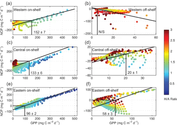
Linear regressions of NCP against GPP were conducted with the aim of estimating threshold GPP, i.e., the GPP value at which NCP becomes positive (Duarte and Regaudie-de-Gioux, 2009). Here, threshold GPPs were used as further indicators of the spatial variability of heterotrophy vs. au-totrophy across the Mackenzie Shelf. Given that GPP and NCP are both dependent variables, regressions were com-puted using a model II least squares bisector equation (Ge-ometric Mean Functional Relationship; Sprent and Dolby, 1980). These linear models determine the slope of the line (through the centroid) that bisects the minor angle between the regressions of Y-on-X and X-on-Y. The Matlab function
lsqbisec (Peltzer, 2008) was used to compute the model II
least squares bisector regressions.
3 Results
In addition of the results presented here, we refer the reader to the supplementary material available online. This supple-mentary material presents a detailed summary of all key re-sults from the gridded maps produced in the framework of our synthesis study.
3.1 Overview of sea ice, wind and satellite-derived
primary productivity
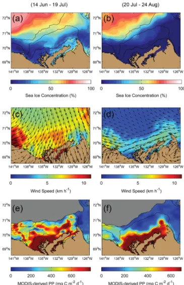
Sea ice and wind conditions in summer 2009 in the Beaufort Sea were influenced by a shift in the atmospheric pattern that occurred between July and August. Over the early summer, the region was affected by a high-pressure system (anticy-clone) located around 70◦N 156◦W that brought clear-sky
conditions, southward advection of old sea ice from the Arc-tic pack (Fig. 3a), and persistent northerly winds (Fig. 3c). In early August, the atmospheric conditions that were observed in the months of June and July collapsed and the mid-to-late summer season was characterized by a low-pressure system that caused cloudy conditions. This cyclone had a catalytic effect on the melt of sea ice through the dispersal of ice floes,
which resulted in what can be seen in Fig. 3b – i.e., large ar-eas of open water over the Mackenzie Shelf and a maximum ice concentration of ∼ 80 % over the deep basin. The mean wind pattern observed over the field campaign (Fig. 3d) was computed as a weak easterly wind (< 5 km h−1), which was a result of the disruption of the anticyclone.
Remote sensing estimates of PP (Fig. 3d and e) showed that PP appeared to be primarily intertwined with the Mackenzie River plume that propagated westward along the Alaskan coast under the influence of northerly winds in June–July. Hence, given the easterly wind pattern that was calculated for late July–August, turbid waters from the Mackenzie River had, presumably, no impact at all on PP es-timates east of Kugmallit Valley or Canyon in summer 2009.
3.2 Sea surface physics, inorganic carbon and sea-to-air
CO2fluxes
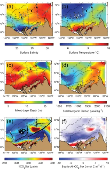
The trajectory of the Mackenzie River plume during July– August was clearly visible on the map of sea surface salinity (Fig. 4a). This confirmed that the eastern portion of the study area was not influenced by any substantial freshwater input. Even surface waters on the eastern shelf remained around a salinity of 30, which is not a particularly low value for the Beaufort Sea. Surface waters with a salinity < 20 were restricted to the inner shelf close to the Mackenzie delta. Brackish surface waters were also generally characterized by increased temperature (up to ∼ 10◦C in very shallow waters, Fig. 4b). Near-0◦C surface waters were associated with the presence of sea ice and a transition from 0◦C to 10◦C was measured as the distance to the ice edge increased.
The vertical extent of the MLD generally increased as sea surface salinity increased and as temperature decreased (Fig. 4c). There was no clear difference between stations af-fected by the absence or presence of sea ice. Mapping of MLDs showed that the mouth of the Amundsen Gulf was the zone where the MLD extended the deepest (down to ∼ 17 m), but MLD values were small overall, with a mean ± standard deviation (SD) of 8.1 ± 3.1 m for the whole study area. Here, MLDs were used to delimit the surface and subsurface lay-ers.
Gridded concentrations of TIC at the ocean surface showed a clear gradient from west to east (Fig. 4d). TIC concentrations were significantly (p < 0.01) related to salin-ity (S) in the mixed layer (TIC = 48.4 × S + 562.6; r2=0.88;
n =77) if we omit data strongly influenced by the Mackenzie River plume (i.e., the inner shelf)
The spatial variability of CO2 fugacity at the sea sur-face was high (ranging from 198 to 660 µatm, mean ± SD of 322 ± 60 µatm), with marked maxima on the outer eastern shelf, near the Mackenzie River delta and toward the Alaskan coast, and to some extent in the Amundsen Gulf (Fig. 4e).
The computation of sea-to-air CO2fluxes revealed that the zones affected by elevated CO2 fugacity were the only re-gions acting as sources of carbon to the atmosphere (Fig. 4f),
Figure 3. Composites of (a, b) sea ice concentration (% ice
cov-erage) from the SSM/I-DMSP orbiting sensor, (c, d) wind velocity and vectors from the NCEP-NARR reanalysis, and (e, f) rates of primary production (PP) derived from the MODIS satellite, as aver-aged for the 35-day period just before (14 June–19 July, left panels) and just during (20 July–24 August, right panels) the ArcticNet– Malina field campaign. The grayscale masks in panels (e, f) depict the areas where no satellite pixels could be extracted from the dis-crete MODIS images because of the presence of sea ice. Bathymet-ric contours are 20, 100 and 1000 m.
especially the river delta (up to ∼ 20 mmol C m−2d−1) and the localized hotspot northwest of Cape Bathurst (up to
∼10 mmol C m−2d−1). Other areas were acting as a car-bon sink, with maximum drawdown of CO2on the mid-to-outer shelf north of the Mackenzie River delta and near the Banks Island shelf (down to ∼ −10 mmol C m−2d−1). Over-all, the southeastern Beaufort Sea acted as a weak sink of atmospheric CO2 in July–August 2009 with a mean uptake of −2.0 ± 3.3 mmol C m−2d−1.
Figure 4. Gridded composites of in situ physico-chemical data
ob-tained at the sampling stations (white dots) conducted in the Beau-fort Sea in mid-summer 2009 (Fig. 1): (a) surface salinity, (b) sur-face temperature, (c) depth of the mixed layer delimiting the sursur-face and subsurface layers as used in this study, (d) concentration of dis-solved inorganic carbon, (e) sea surface CO2 fugacity (combined
data set from the underway system and bottle data), and (f) the sea-to-air CO2fluxes (blue: flux to the ocean; red: to the atmosphere) as
computed following the methodology described in Sect. 2.3. Bathy-metric contours are 20, 100, 1000, and 2000 m. The region close to Cape Bathurst on the eastern shelf is known to be a region where wind-driven upwelling is enhanced by the steep topography (see Williams and Carmack, 2008).
3.3 Bulk budget of organic carbon pools, river inputs
and vertical fluxes
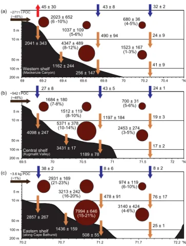
We developed a non-steady-state budget of bulk carbon fluxes and pools for the Mackenzie Shelf in July–August 2009 (Fig. 5) using estimates of organic carbon inputs from the Mackenzie River and Anderson River, POC and DOC measurements in the water column, and vertical POC fluxes. The budget summary is presented as spatial averages across the western, central and eastern zones of the study area as
delimited by 136–141◦W, 131–136◦W and 126–131◦W,
re-spectively.
The main result of this bulk budget is the fact that POC inventories were overall higher on the eastern shelf than on the central and western shelf, despite the tremendous POC input from the Mackenzie River, which delivered a daily average load of 3253 ± 2183 t POC d−1 in these two zones combined. The mean total inventory of POC (inte-grated vertically, sum of the surface and subsurface layers) in the eastern region (Fig. 5c) was 18.3 ± 1.5 g C m−2, whereas it was 9.6 ± 1.0 g C m−2 in the western zone (Fig. 5a) and 11.7 ± 1.6 g C m−2in the central region (Fig. 5b). Similarly, the quantity of POC relative to ambient DOC roughly dou-bled from west to east (from ∼ 6.0 % to ∼ 13.7 %; Fig. 5). This suggests that DOC concentrations remain relatively the same across the study area when integrated vertically in the upper 100 m.
A second key result of this summary concerns ver-tical POC fluxes that did not follow the same pat-tern as POC inventories. When averaged across the three zones, mean vertical POC fluxes were higher in the central zone (1790 ± 122 mg C m−2d−1), compared against the eastern (897 ± 98 mg C m−2d−1) and western (669 ± 141 mg C m−2d−1) regions. In addition, vertical POC fluxes injected into the benthic boundary layer (as derived from UVP5 recordings) were particularly high on the inner-mid shelf (< 60 m isobath, ∼ 1200–4100 mg C m−2d−1) when compared to the relatively low POC inventories found in shallow waters (∼ 1600–2900 mg C m−2), implying that the residence time of POC in the water column near the coast is very low and/or that the area is affected by resuspension. Overall, estimates of vertical POC fluxes over the shelf were one to two orders of magnitude greater than offshore.
3.4 Nutrient dynamics, phytoplankton biomass and
primary production
During ArcticNet–Malina 2009, nitrate represented 96.6 % of the total nitrogenous nutrient concentrations in the up-per 100 m, while nitrite and ammonium accounted for 1.4 and 2.0 %, respectively. In surface waters, nitrate concentra-tions were typically lower than 0.01 µM, except close to the Mackenzie River delta, where undiluted freshwater with a nitrate of 3.6 µM was found. Below the surface mixed layer (Fig. 4c), nitrate remained depleted typically down to 40– 50 m depth, followed by a clear nitracline associated with the increasing presence of Pacific-derived waters that occu-pied the 50–200 m layer. A three-dimensional view of nitrate concentrations (as measured at the Malina cross-shelf tran-sects) provided synoptic insights on the geographical and vertical variability of the nitracline during our study (Fig. 6). In this figure, we can observe a clear cross-shelf structure of nitrate-rich waters that propagated inshore within the bottom 10–15 m of the water column. This oblique expansion (along the isopycnals) of the nitracline from the basin to the shelf
69 69.2 69.4 69.6 69.8 70 70.2 70.4 69.5 70 70.5 71 71.5 72 70.2 70.7 71.2 71.7 72.2 10 m 100 m 200 m 5 m 50 m 10 m 100 m 200 m 5 m 50 m 10 m 100 m 200 m 5 m 50 m °N °N °N 2023 ± 652 (6 -10%) 1684 ± 180 (7-8%) 2931 ± 169 (21-23%) 1037 ± 109 (5-6%) 1512 ± 119 (8-10%) 680 ± 36 (4-5%) 700 ± 31 (5-6%) 3213 ± 242 (16-20%) 974 ± 119 (6-10%) 4347 ± 489 (8-12%) 1523 ± 167 (1-3%) 5371 ± 378 (10-14%) 2453 ± 274 (3-5%) 7994 ± 646 (15-21%) 3140 ± 424 (4-6%) 2041 ± 343 4098 ± 247 2857 ± 267 1162 ± 244 490 ± 94 24 ± 9 1197 ± 184 19 ± 3 478 ± 91 76 ± 17 41 ± 9 17 ± 2 25 ± 1 3431 ± 17 1436 ± 159 256 ± 147 1189 ± 78 508 ± 55 ~2711 t POC (~48%) ~542 t POC (~48%) ~3.6 kg POC (~1%) 45 ± 30 43 ± 8 32 ± 2 27 ± 8 43 ± 5 24 ± 1 38 ± 2 8 ± 6 8 ± 2 Western shelf (Mackenzie Canyon) Central shelf (Kugmallit Valley) Eastern shelf (along Cape Bathurst)
(a)
(b)
(c)
Figure 5. Cross-shelf averages (mean ± 0.95 confidence interval)
of particulate organic carbon (POC) inventories (dark brown cir-cles), vertical POC fluxes (light brown arrows), riverine POC inputs (black arrows), and sea-to-air CO2fluxes (red and dark blue
ar-rows). All pool units (circles) are in mg C m−2and all flux units (arrows) are in mg C m−2d−1, except the riverine inputs (which are in tons or kg per day). The percentage in brackets associated with every POC inventory and river input is the fraction of POC in total organic carbon (particulate + dissolved) that each value represents. The western, central and eastern regions correspond to the areas de-limited by 136–141◦W, 131–136◦W and 126–131◦W, respectively (Fig. 1). For a detailed description on how each variable has been estimated, please see Sect. 2.4.
was particularly visible at transects conducted north of Cape Bathurst and in the Mackenzie Canyon. In the head of the canyon, we estimated using Delaunay triangulation that wa-ters just below the surface contained nitrate concentration up to 6–7 µM (Fig. 6).
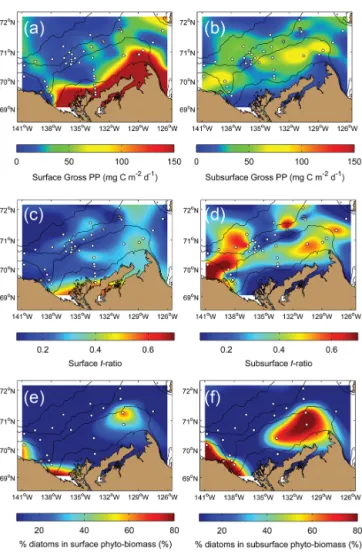
Relatively high GPP rates (∼ 200–500 mg C m−2d−1; based on on-deck incubations) during our field survey were confined to the surface (above MLD) inshore en-vironment (within the 20 m isobath) and to some extent to the mid-shelf region close to Cape Bathurst (Fig. 7a). Elsewhere, GPP in surface waters remained at very low levels (∼ 10–50 mg C m−2d−1). Beyond the inner shelf, GPP was actually higher below the surface (below MLD) than within the surface mixed layer, with rates up to
Figure 6. Three-dimensional view of the Mackenzie Shelf region
showing the nitrate concentration as measured at transects 100, 200, 300, 400, 600 and 700 (from left to right) during the Malina expedi-tion (Fig. 1). Each vertical slice corresponds to a gridded compos-ite of nitrate concentration measured at standard depths along the cross-shelf sampling line.
75–90 mg C m−2d−1. When spatially averaged over the whole study area (∼ 140.1 × 10³km2), GPP in the sur-face layer was 55.9 ± 82.7 mg C m−2d−1, which represented on the average 62.6 % of the total GPP in the upper 100 m (89.2 ± 102.1 mg C m−2d−1). Using a study period of 35 days for ArcticNet–Malina, this yielded a cumulated GPP of 3.1 ± 3.6 g C m−2. It also provided a total GPP for the whole study region of ∼ 437.6 × 10³t C, which was roughly twice the total organic carbon delivery (POC + DOC) by the Mackenzie and Anderson River (∼ 241.2 × 10³t C) from 20 July to 24 August 2009.
The ratios of new production to total GPP (f ratio, as based on nitrate and ammonium uptake) were relatively low in the surface layer (∼ 0.2), except close to Cape Bathurst (∼ 0.4) and near the Mackenzie River delta (∼ 0.6), which re-flected localized sources of nitrate from upwelling and river-ine input, respectively (Fig. 7c). Below the surface mixed layer, f ratios were also very variable, but relatively high
f ratios (> 0.6) were found along the Alaskan coast, close to Cape Bathurst and at few locations offshore (Fig. 7d). At some stations west of the Mackenzie Canyon and on the outer eastern shelf, diatoms overwhelmingly dominated (> 80 %) phytoplankton biomass. At stations where the abundance of diatoms was low, autotrophic flagellates dominated the phy-toplankton assemblage (not shown).
Further details on the geographic and vertical variability of phytoplankton biomass (B) and production (P ) are presented in Table 1. This enables us to calculate an ensemble of P : B ratios. Highest P : B ratios (up to ∼ 41 % d−1) were found within the surface mixed layer, whereas P : B ratios found in association with subsurface productivity were 5–10 times lower (Table 1).
T able 1. Spatial av erages (mean ± 0.95 confidence interv al) of biomass (B ), production (P ), and P : B ratios (e xpressed in % per day), of pelagic autotrophs (ph ytoplankton) and heterotrophs (bacteria, protozoans and metazooplankton) as estimated from the ArcticNet–Malina data set collected o v er July– August 2009 in southeast Beaufort Sea (Fig. 1). The mean mix ed-layer depth delimits the bound ary between the surf ace and subsurf ace layer . The subsurf ace layer extends do wn to 100 m maximum. The threshold between the on-shelf and of f-shelf re gion is the 100 m isobath. The western, central and eastern re gions correspond to the areas delimited by 136–141 ◦W , 131–136 ◦W and 126–131 ◦W , respecti v ely . Surf ace (abo v e mix ed-layer depth) Subsurf ace (belo w mix ed-laye r depth until 100 m) On-shelf re gion Of f-shelf re gion On-shelf re gion Of f-shelf re gion W estern Central Eastern W estern Central Eastern W estern Central Eastern W estern Central Eastern Ph ytoplankton Production (mg C m − 2d − 1) 63.4 ± 13.5 68 .2 ± 9.6 15 3 ± 13 15.8 ± 1.2 12.0 ± 1.1 43 .3 ± 3.8 32.1 ± 3.1 37.4 ± 1.9 3 7.2 ± 3.4 40.5 ± 1.8 26. 8 ± 1.8 25.5 ± 1.3 Biomass (mg C m − 2) 264 ± 36 328 ± 20 374 ± 13 69.6 ± 3.8 64.1 ± 4.1 128 ± 7 795 ± 55 767 ± 40 148 0 ± 54 341 ± 11 535 ± 23 6 86 ± 27 P : B ratio (% per day) 24.0 ± 3.6 2 0.8 ± 1.6 40.8 ± 2.0 22.7 ± 1.3 18.8 ± 1.3 33 .8 ± 2.1 4.0 ± 0.3 4.9 ± 0.3 2.5 ± 0.1 11.9 ± 0.4 5 .0 ± 0.2 3.7 ± 0.1 Bacteria Production (mg C m − 2d − 1) 18.0 ± 2.8 18 .6 ± 1.9 22.2 ± 1.0 3.1 ± 0.5 1.5 ± 0.2 7 .4 ± 0.6 25.8 ± 4.1 19.5 ± 1.4 2 4.9 ± 2.0 9.3 ± 0.6 5. 7 ± 0.5 12.2 ± 1.2 Biomass (mg C m − 2) 126 ± 4 12 0 ± 5 82.9 ± 3.7 74.7 ± 4.4 37.1 ± 2.2 67 .3 ± 4.3 437 ± 36 328 ± 12 24 1 ± 27 557 ± 14 496 ± 22 7 32 ± 49 P : B ratio (% per day) 14.3 ± 0.7 1 5.5 ± 0.8 26.8 ± 1.2 4.1 ± 0.3 3.9 ± 0.2 11 .0 ± 0.7 5.9 ± 0.5 5.9 ± 0.2 10.3 ± 1.1 1.7 ± 0.0 1 .2 ± 0.1 1.7 ± 0.1 Protozooplankton Production (mg C m − 2d − 1) 28.5 ± 3.9 19 .1 ± 1.7 5.7 ± 0.4 6.6 ± 0.5 5.1 ± 0.3 6 .1 ± 0.4 19.6 ± 0.6 15.2 ± 0.4 1 5.2 ± 0.6 17.2 ± 0.8 22. 9 ± 0.9 22.6 ± 1.0 Biomass (mg C m − 2) 333 ± 34 167 ± 12 93.1 ± 5.1 95.4 ± 6.9 84.7 ± 4.1 110 ± 3 335 ± 10 257 ± 5 2 73 ± 4 284 ± 15 378 ± 13 3 51 ± 12 P : B ratio (% per day) 8.6 ± 0.9 1 1.4 ± 0.9 6.2 ± 0.3 6.9 ± 0.5 6.1 ± 0.3 5 .6 ± 0.2 5.9 ± 0.2 5.9 ± 0.1 5.6 ± 0.1 6.1 ± 0.3 6. 1 ± 0.2 6.4 ± 0.2 Nauplii & small Production (mg C m − 2d − 1) 0.2 ± 0.0 1 .6 ± 0.1 1.5 ± 0.1 0.1 ± 0.0 0.1 ± 0.0 0 .2 ± 0.0 0.6 ± 0.1 6.4 ± 0.5 6.1 ± 0.6 0.8 ± 0.1 1.6 ± 0.2 1.6 ± 0.2 metazooplankton Biomass (mg C m − 2) 13.9 ± 2.2 68 .3 ± 5.2 69.1 ± 5.5 3.2 ± 0.4 5.3 ± 1.4 8 .5 ± 1.0 21.9 ± 4.0 274 ± 23 21 5 ± 18 36.9 ± 3.2 78.6 ± 10.7 73.4 ± 7.3 P : B ratio (% per day) 1.3 ± 0.2 2 .3 ± 0.2 2.1 ± 0.2 2.1 ± 0.3 2.1 ± 0.6 2 .2 ± 0.3 2.8 ± 0.5 2.3 ± 0.2 2.8 ± 0.2 2.2 ± 0.2 2. 0 ± 0.3 2.2 ± 0.2 Lar ge metazooplankton Production (mg C m − 2d − 1) 0.2 ± 0.0 0 .5 ± 0.0 1.5 ± 0.1 0.1 ± 0.0 0.2 ± 0.0 0 .5 ± 0.1 1.9 ± 0.2 19.7 ± 1.6 1 6.7 ± 1.2 4.4 ± 0.3 7. 9 ± 0.6 9.9 ± 0.6 Biomass (mg C m − 2) 17.8 ± 2.4 38 .9 ± 3.7 13 9 ± 13 4.1 ± 0.4 13.0 ± 2.0 47 .5 ± 4.9 86.2 ± 32.3 1820 ± 149 1603 ± 143 519 ± 30 1004 ± 55 105 2 ± 100 P : B ratio (% per day) 1.3 ± 0.2 1.2 ± 0.1 1.1 ± 0.1 1.3 ± 0.1 1.2 ± 0.2 1 .1 ± 0.1 2.2 ± 0.8 1.1 ± 0.1 1.0 ± 0.1 0.9 ± 0.0 0. 8 ± 0.0 0.9 ± 0.1 T otal heterotrophs Production (mg C m − 2d − 1) 46.8 ± 6.8 39 .8 ± 3.7 31.0 ± 1.8 9.7 ± 1.1 6.9 ± 0.5 14 .2 ± 1.1 47.9 ± 5.0 60.7 ± 3.9 6 2.9 ± 4.3 31.7 ± 1.7 38. 2 ± 2.2 46.3 ± 2.8 Biomass (mg C m − 2) 491 ± 43 395 ± 26 384 ± 28 177 ± 12 14 0 ± 10 233 ± 13 880 ± 83 26 80 ± 190 2332 ± 193 1397 ± 63 1956 ± 101 220 9 ± 168 P : B ratio (% per day) 9.5 ± 0.9 1 0.1 ± 0.7 8.1 ± 0.6 5.5 ± 0.4 4.9 ± 0.3 6 .1 ± 0.4 5.4 ± 0.5 2.3 ± 0.2 2.7 ± 0.2 2.3 ± 0.1 2. 0 ± 0.1 2.1 ± 0.2 T otal heterotroph-to-autotroph produ ction ratio (unitless) 0.74 ± 0.14 0.5 8 ± 0.07 0.20 ± 0.02 0.62 ± 0.06 0 .57 ± 0.05 0.33 ± 0.03 1.49 ± 0.15 1.63 ± 0.10 1. 69 ± 0.13 0.78 ± 0.04 1.42 ± 0.09 1.81 ± 0.10 T otal heterotroph-to-autotroph biomass ratio (unitless) 1.86 ± 0.19 1.2 0 ± 0.08 1.03 ± 0.05 2.55 ± 0.16 2 .18 ± 0.15 1.82 ± 0.10 1.11 ± 0.09 3.49 ± 0.23 1. 58 ± 0.10 4.09 ± 0.17 3.66 ± 0.18 3.22 ± 0.22
Figure 7. Gridded composites of variables related to phytoplankton
dynamics as measured in the surface and subsurface layer of the study region: (a, b) total gross primary production (PP) from field measurements, (c, d) the f ratio of new PP to total PP as estimated on the basis of nitrate and ammonium uptake incubations, and (e, f) the percentage of diatoms in the total phytoplankton biomass. The white dots correspond to the sampling sites. Bathymetric contours are 20, 100, 1000, and 2000 m.
3.5 Biomass, production and respiration of bacteria,
zooplankton and benthos
Estimates (and 95 % confidence intervals) of biomass and secondary production of pelagic heterotrophs are listed in Table 1. Secondary production within the surface layer was equally dominated by protozoans (48 %) and bacteria (47 %), while metazooplankton (sum of the two size-fractions) ac-counted for 5 %. Below the surface layer, metazooplank-ton represented 28 % of the secondary production, whereas bacteria and protozoans contributed on the average to 33 and 39 %, respectively. Relative biomass of heterotrophs in the surface layer was more homogenous than their produc-tion (i.e., protozoans 48 %, bacteria 29 %, metazooplankton, 24 %). Below the surface, protozoans and bacteria accounted
for 16 and 24 %, while metazooplankton dominated the total heterotroph biomass at 60 %. It is worth mentioning that the biomass of metazooplankton was roughly 300 % greater in the central and eastern zones than in the western region of the study area, which was affected by the Mackenzie River plume. A spatial match between the biomass of metazoo-plankton and phytometazoo-plankton was detected in the eastern on-shelf subsurface layer where these two groups accounted for 87 % of the whole plankton biomass.
Unsurprisingly, bacteria and protozooplankton had higher
P : Bratios (range ∼ 1.2–26.8 % d−1) than metazooplankton
(range ∼ 0.8–2.8 % d−1), likely because of their low struc-tural carbon content (i.e., high carbon turnover capacity). The highest bacterial P : B ratio (∼ 26.8 % d−1) was found in the surface layer of the eastern on-shelf region, while the pro-duction of protozoans relative to their biomass was strongest (∼ 11.4 % d−1) in the central on-shelf zone. Interestingly, the
P : Bratios of protozoans was ca. 3 times higher than that of
bacteria in the subsurface layer off the shelf, contrary to what was seen in other areas (Table 1).
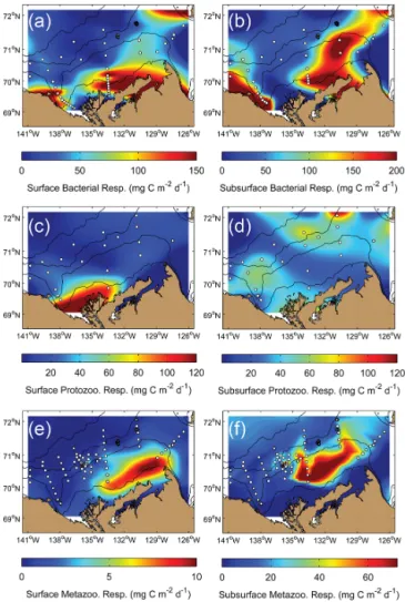
The gridded maps of respiration fluxes (Fig. 8) com-plemented the biomass and production data of Table 1 by providing an overview of the spatial variability of het-erotrophic activity. When averaged over the whole study area (see definition in Sect. 2.7), respiration outflows from bacteria in the surface and subsurface layers (48 ± 44 and 87 ± 88 mg C m−2d−1, respectively) were both statistically greater (Mann–Whitney U test, p < 0.001) than those of pro-tozoans (23 ± 30 and 38 ± 14 mg C m−2d−1, respectively), which were themselves both statistically higher (same test and p value) than those of total metazooplankton (2 ± 3 and 23 ± 21 mg C m−2d−1). Therefore, an interesting feature that we can discern from the respiration maps is the emer-gence of an anti-correlation pattern between respiration by bacteria and respiration by protozoans (Fig. 8a and b vs. Fig. 8c and d); and between respiration by protozoans and respiration by metazooplankton (Fig. 8c and d vs. Fig. 8e and f). For example, protozoan activity was high in the Macken-zie River delta, a zone where bacterial respiration was sur-prisingly low. Similarly, protozoan respiration was low on the central and eastern shelf, exactly where metazooplankton activity was greatest.
Estimates of benthic respiration on the shelf (derived from field measurements) are presented in Fig. 9. Respiration rates were converted to production rates, which yielded val-ues ranging from 15–40 mg C m−2d−1. Further estimates of epifaunal benthic biomass on the shelf (using an empirical model, see Sect. 2.6) lead to a range of ∼ 3.4–8.9 g C m−2. This implies that, on the average, benthic biomass was at least more than twice (∼ 5.9 g C m−2) the cumulated biomass of pelagic heterotrophs in the surface and subsurface lay-ers on the shelf (∼ 2.4 g C m−2), although pelagic organisms overwhelmingly dominated (∼ 88%) total respiration fluxes (Fig. 9).
Figure 8. Gridded composites of estimated values related to
het-erotroph respiration in the surface (left panels) and subsurface (right panels) layer: (a, b) bacterial respiration, (c, d) protozooplankton respiration, and (e, f) metazooplankton respiration. The white dots correspond to the sampling stations upon which respiration esti-mates were calculated. For a detailed description on how each res-piration flux has been estimated, please see Sect. 2.6.
3.6 Ecosystem metabolic balance and net community
production estimates
The ecosystem metabolic balance, as being defined as the in-terplay between GPP and CR, is depicted schematically in Fig. 9 and via the surface and subsurface gridded maps of Fig. 10. The cross-shelf averages of GPP and respiration out-flows (Fig. 9) aim at simplifying the large spatial variability presented in Figs. 7 and 8. As seen above, bacteria domi-nated the overall organic carbon remineralization across the study region, but protozoans were important players near the Mackenzie River delta and beyond the shelf break. The im-portance of metazooplankton was only really noticed in the subsurface layer of the central and eastern regions (Fig. 9b and c). 69 69.2 69.4 69.6 69.8 70 70.2 70.4 69.5 70 70.5 71 71.5 72 70.2 70.7 71.2 71.7 72.2 10 m 100 m 200 m 5 m 50 m 10 m 100 m 200 m 5 m 50 m 10 m 100 m 200 m 5 m 50 m °N °N °N 104 ± 12 36 ± 4 94 ± 9 20 ± 5 91 ± 5 63 ± 6 28 ± 6 16 ± 1 29 ± 3 12 ± 1 96 ± 9 43 ± 4 193 ± 25 101 ± 6 294 ± 13 99 ± 6 219 ± 16 139 ± 10 37 ± 2 27 ± 2 32 ± 3 41 ± 2 37 ± 3 26 ± 1 203 ± 31 220 ± 19 144 ± 10 94 ± 12 84 ± 2 52 ± 3 66 ± 3 35 ± 9 41 ± 2 45 ± 30 43 ± 8 32 ± 2 27 ± 8 43 ± 5 24 ± 1 38 ± 2 8 ± 6 8 ± 2 8 Western shelf (Mackenzie Canyon) Central shelf (Kugmallit Valley) Eastern shelf (along Cape Bathurst)
(a) (b) (c) 12 Auto Hetero smallZoo 8 4 174 ± 26 264 ± 21 172 ± 36
Figure 9. Cross-shelf average estimates (mean ± 0.95 confidence
interval) of gross primary production (green circles), total pelagic heterotroph respiration (pie charts), benthic respiration (orange cir-cles in the sediment), and sea-to-air CO2fluxes (red and dark blue
arrows; same as in Fig. 4). Every pie chart represents the com-bined respiration of phytoplankton (green), bacteria (dark blue), protozooplankton (dark orange), small metazooplankton and nau-plii (dark red), and large metazooplankton (yellow). All units are in mg C m−2d−1. The western, central and eastern regions corre-spond to the areas delimited by 136–141◦W, 131–136◦W and 126– 131◦W, respectively (Fig. 1). For a detailed description on how each variable has been estimated, please see Sects. 2.5 and 2.6.
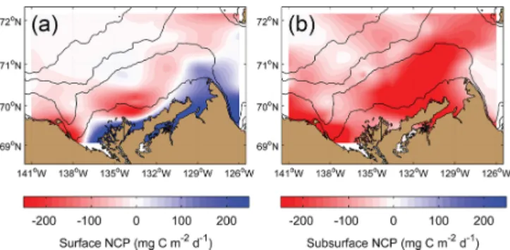
Generally, respiration in the surface mixed layer exceeded GPP, which resulted in the NCP map shown in Fig. 10a. Surface NCP was clearly positive only near to shore and around Cape Bathurst, where increased GPP has been esti-mated through both remote sensing (Fig. 3f) and in situ field measurements (Fig. 7a). However, surface NCP was close to zero and/or slightly positive in some regions affected by the persistent presence of sea ice (Fig. 3b). Below the sur-face layer down to 100 m depth, NCP was negative every-where (Fig. 10b) with a signal dominated by BR (Fig. 8b). When averaged for the whole region, NCP in the surface and subsurface layer was −22.6 ± 70.6 mg C m−2d−1 and