HAL Id: hal-01242608
https://hal.archives-ouvertes.fr/hal-01242608
Submitted on 24 Apr 2016
HAL is a multi-disciplinary open access
archive for the deposit and dissemination of
sci-L’archive ouverte pluridisciplinaire HAL, est
destinée au dépôt et à la diffusion de documents
Externalisation of Time-Triggered communication
system in BIP high level models
Hela Guesmi, Belgacem Ben Hedia, Simon Bliudze, Saddek Bensalem
To cite this version:
Hela Guesmi, Belgacem Ben Hedia, Simon Bliudze, Saddek Bensalem. Externalisation of
Time-Triggered communication system in BIP high level models. 8th Junior Researcher Workshop on
Real-Time Computing (JRWRTC 2014), Oct 2014, Versailles, France. pp.47-50. �hal-01242608�
Externalisation of Time-Triggered communication system
in BIP high level models
Hela Guesmi, Belgacem
Ben Hedia
CEA, LIST[email protected]
Simon Bliudze
EPFL[email protected]
Saddek Bensalem
Verimag, UJF[email protected]
ABSTRACT
To target a wider spectrum of Time-Triggered(TT) imple-mentations of hard real-time systems, we consider approaches for building component-based systems that provide a phys-ical model from a high-level model of the system and TT specifications. The obtained physical model is thus suitable for direct transformation into languages of specific TT plat-forms. In addition, if these approaches provide correctness-by-construction, they can help to avoid the monolithic a posteriori validation.
In this paper, we focus on the TT interface concept of the TT paradigm. And we present a method that transforms the interaction in classic BIP (Behavior, Interaction, Prior-ity) Model into a TT interface by source-to-source transfor-mations. The method is based on the successive application of two types of source-to-source transformations; Transfer functions internalisation and n + 1-ary connector to TT in-terface transformation. The first simplifies the connector transfer functions by modifying components automata. The second transforms connector with simple transfer function into TT interfaces.
Keywords
TT paradigm; correctness-by-construction; Source-to-source transformation; BIP; interaction expressions; connectors;
1. INTRODUCTION
In hard real time computer systems, correctness of a re-sult depends on both the time and the value domains. With the increasing complexity of these systems, ensuring their correctness using a posteriori verification becomes, at best, a major factor in the development cost and, at worst, simply impossible. An error in the specifications is not de-tectable. We must, therefore, define a structured and simpli-fied design process which allows the development of correct-by-construction system. Thereby, monolithic a posteriori verification can be avoided as much as possible.
Two fundamentally different paradigms for the design of real-time systems are identified; Event-Triggered(ET) and TT paradigms. In ET paradigm, all communication and processing activities are initiated whenever a considerable event, i.e., change of state in the observed variable, is no-ticed. It doesn’t cope with demands for predictability and determinism that must be met in hard real-time systems. Activities in TT paradigm are initiated periodically at pre-determined points in time. These statically defined activa-tion instants enforce regularity and make TT systems more predictable than ET systems. This approach is well-suited for hard real-time systems.
A system model of this paradigm is essential to speed-up understanding and smooth design task. It requires explic-itly manipulating not only the value domain specifications,
but also temporal constraints for which high abstraction level primitives are not provided. Kopetz [7] presents a TT-Model of computation, based on essential properties of the TT paradigm: the global notion of time that must be established by a periodic clock synchronization in order to enable a TT communication and computation, the tempo-ral structure of each task, consisting of predefined start and worst-case termination instants attributed statically to each task and TT interfaces which is a memory element shared between two interfacing subsystems. TT-Model sep-arates the design of interactions between components from the design of the components themselves.
To target a wider spectrum of TT implementations, we consider approaches for building component-based systems that provide a physical model from a high-level model of the system and TT specifications. In addition, if these ap-proaches provide correctness-by-construction, they can avoid the monolithic a posteriori validation. We focus in particu-lar on the framework BIP [1]. It is a component framework for constructing systems by the superposition of three lay-ers: Behaviour, Interaction, and Priority. The Behaviour layer consists of a set of atomic components represented by transition systems. The second layer describes possible in-teractions between atomic component. Inin-teractions are set of ports and are specified by a set of connectors. The third layer includes priorities between interactions using mecha-nisms for conflict resolution. In this paper, we consider Real-Time BIP version [2] where atomic components are repre-sented by timed automata. We limit ourselves to connectors and leave priorities for future work.
From a high-level BIP system model, a physical model containing all TT concepts (such as TT interfaces, the global notion of time and the temporal structure of each task) is generated using a set of source-to-source transformations. This physical model (called also BIP-TT model) is then translated to the programming language specific to the par-ticular TT platform. The program in this language is then compiled using the associated compilation chain. Thus, BIP-TT model is not dedicated to an exemplary architecture.
There have been a number of approaches exposing the rel-evant features of the underlying architectures at high level design tool. [8] presents a design framework based on UML diagrams for applications running on Time Triggered Ar-chitecture(TTA). This approach doesn’t support earlier ar-chitectural design phase and needs a backward mechanisms for the generated code verification. Since BIP design flow is unique due to its single semantic framework used to support application modelling and to generate correct-by-construction code, many approaches tend to use it to translate high level models into physical models including architectural features. In [5], a distributed BIP model is generated from a high level
one. In [4], a method is presented for generating a mixed hardware/software system model for many-core platforms from an application software and a mapping. These two ap-proaches take advantages from BIP framework but they do not address the TT paradigm. To the best of our knowl-edge, our approach is the first to address the problem of generating TT application from BIP high level models.
In this paper we address the issue of source-to-source transformations that explicit TT communications in the phys-ical model, in BIP framework. Other TT concepts ( the global synchronized time and task temporal structure) trans-formations are beyond the scope of this paper.
The remainder of this paper is structured as follows: Sec-tion 2 introduces BIP framework and explains the relevant TT concepts. Section 3, presents a method using a set of source-to-source transformations for generating a BIP model expliciting TT communication interfaces, from a high level classic BIP model. In Section 4, we conclude the paper by discussing advantages and downsides of our method.
2. RELATED CONCEPTS
In this section, we present first the basic semantic model of BIP, and main TT concepts that must clearly appear in the final BIP-TT model.
2.1 The BIP component framework
In the BIP framework, for each layer, a concrete model is provided. Atomic components model the behaviour layer. The interaction layer is modelled with connectors and finally Priorities is a mechanism for scheduling interactions.
An atomic component consists of a timed automaton with local data and an interface consisting of ports. Transitions in the component automaton are labelled by ports and can execute C code to transform local data. LetP be a set of ports. We assume that every port p∈ P has an associated data variable xp. This variable is used to exchange data
with other components, when interactions take place. Definition 1. (atomic component):
An atomic component B is defined by B = (L, P, T, X, {gτ}τ∈T,{fτ}τ∈T), where,
• (L, P, T ) is a labelled transition system, that is: – L is a set of control states
– P is a set of communication ports, – T⊆ L × 2P× L is a set of transitions
• X is a set of variables and for each transition τ ∈ T , gτis a guard and fτis an update function that is state
transformer defined on X.
Interactions which are sets of ports allowing synchroniza-tions between components, are defined and graphically rep-resented by connectors. The execution of interactions may involve transfer of data between the participating compo-nents. For every interaction, data transfer functions of an interaction a are specified by an U p and a Down actions. The action U p is supposed to update the local variables of the connector, using the values of variables associated with the ports. Conversely, the action Down is supposed to up-date the variables associated with the ports, using the values of the connector variables.
Definition 2. (Connector) A connector γ defines sets of ports of atomic components Biwhich can be involved in an
interaction a. It is formalized by γ = (P, a, q, g, U p, Down) where:
• P is the support set of synchronized ports of γ with P = a
• q is its exported port.
• g is the boolean guard expression.
• Up is the upward transfer function of the form xq :=
U p({xp}p∈a),.
• and Down is the downward transfer functions of the form xp:= Downp(xq) for each p∈ a.
The interaction presented by this connector is of the form: (q← a).[g({xp}p∈a) : xq:= U p({xp}p∈a)//xp∈a:=
Downd p(xq)]
2.2 TT Paradigm [6, 7]
TT paradigm encompasses these 3 key concepts; The global synchronized time: It allows definition of
in-stances when communication and computation of tasks take place in a TT system. It is established by a pe-riodic clock synchronization from which other clocks can be derived.
The temporal control structure of the task sequence: The TT paradigm is based on a set of static schedules. These schedules have to provide an implicit synchro-nization of the tasks at run time. This introduces a fixed task activation rates during system design. Thus to each task is allocated predefined start instant (Tb)
and the worst-case termination instant (Te). These
in-stants are triggered by the progression of the global time.
Time-Triggered interface(Firewall): It is a data-sharing boundary between two communicating subsystems. Ex-changed messages are state messages, informing about the state of the relevant variable at a particular point in time. A new version of a state message overwrites the previous version. State messages are not consumed on reading and they are produced periodically at pre-determined points in real-time. Thus TT interfaces contain real-time data which is a valid image of the observed variable.
These three notions should clearly appear in the final BIP-TT model to facilitate its translation into the programming language specific to the particular TT platform.
3. TIME-TRIGGERED ARCHITECTURES
IN BIP
The methodology that integrates TT concepts in BIP, is based on the transformation of an arbitrary BIP model with additional TT annotations (task, TT interfaces) into more restricted models called BIP-TT, which are suitable for di-rect transformation into languages of specific TT platforms. In order to understand the transformation process of a BIP model into BIP-TT one, we present first the original BIP and final BIP-TT models and then we detail the trans-formation rules that transform the former into the latter.
3.1 The original BIP Model
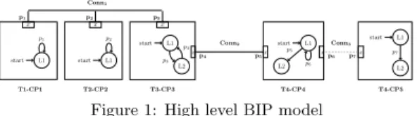
We assume that the considered original BIP model con-sists only of atomic components and flat connectors, exam-ple cf.Figure1. Indeed, these assumptions do not impose restrictions on the components since we can use the ”compo-nent flattening” transformation [5] to replace every compos-ite component by its equivalent set of atomic components.
Figure 1 shows a BIP model, made up of five atomic com-ponents executing four different tasks. We assume that a task is a set of elementary actions. Thus two or more com-ponents can execute separately elementary actions belong-ing to the same task. Each component is annotated by the
L1 start p1 L1 start p2 L1 start L2 p3 p4 start L1 L2 p6 p5 L1 start L2 p7 T1-CP1 T2-CP2 T3-CP3 T4-CP4 T4-CP5 Conn1 Conn2 Conn3 p1 x p2 x p3 x p4 x p5x xp6 p7x
Figure 1: High level BIP model
task it is executing and the component identifier. Take for example the first component, annotated by ”T1-CP1”, i.e., ”CP1” is its identifier and ”T1” is the executed task identi-fier. Two different components may execute the same task, e.g components ”CP4” and ”CP5”. The connector relating such components is shown by dotted lines. To simplify the presentation of figures’ automata in this paper, the temporal aspect is not displayed.
3.2 BIP_TT Model
The final BIP-TT Model presents a hand-made transla-tion of the TT paradigm, introduced by Kopetz, into a BIP model. It clearly includes TT three main concepts. Figure 2b shows roughly how should be the BIP-TT model of the BIP model of Figure 2a. Red components are BIP components and presents TT concepts.
L1 start L2 p1 T1-CP1 L1 start L2 p2 T2-CP2 p1 p2
(a) Original BIP model
L1 start L2 p1 tick T1-CP1 [Tb, Te] L1 start L2 p2 tick T2-CP2 [Tb, Te] p1 p2 Clock System
Global clock Derived clock
tick tick TT in te rfa ce
(b) Final BIP-TT model
Figure 2: Modelling TT paradigm in BIP As here we settle for studying source-to-source transfor-mations to obtain TT interfaces from BIP connectors, we model in Figure 3 the TT interface in BIP. It is an atomic two-port component which behaviour is modelled by a la-belled automaton with one state and two transitions, one for reading action (labelled by the port WIT T) and one for
writing(labelled by the port RIT T).
L WIT T
RIT T
TTinterface WITTx xRITT
Figure 3: BIP model of the TT interface
3.3 Transformations from BIP classic model
to BIP-TT model: from the
communica-tion concept point of view
The high level BIP model refinement process is based on the operational semantics of BIP [3] which allows to com-pute the meaning of a BIP model with simple connectors as a behaviourally equivalent BIP model that contains TT interfaces cf.Figure 3. The transformation process follows these two steps: 1) Transfer functions internalisation and 2) n + 1-ary connector to TT interface transformationFn.
These two transformations are described in reverse, from the most specific to the most general N−ary connector case. We use the high level BIP model in Figure 1 as a running example throughout the paper to illustrate these transfor-mation rules.
3.3.1
n + 1-ary connector to TT interface transfor-mation (Fn)This transformation is applied only on n + 1−ary connec-tor with only one writer, n readers, and with simple
assig-nation transfer functions, i.e., we just copy the value of the associated variable to the writer port in the local variable of the connector (the U p function), and copy the latter in readers’ ports’ variables(Down functions). Note that this behaviour is similar to the TT interface one which is used to make and transfer copy from the producer to consumers. We denote this transformation function byFn, it transforms an
n + 1−ary connector C = (PC, aC, qC, gC, U pC, DownC), in
the source model, into the triplet; binary connector C1, TT
interface IT T, and an n−ary connector C2n, in the resulting
model. These are defined below in function of the initial connector C. Let PCbe the set of ports of the connector C
such as PC={pWC,{pRCi}i∈[1..n]}.
Rule 1. C1
C1is formalized by C1= (P1, a1, q1, g1, U p1, Down1). The
interaction presented by this connector is then of the form: (q1← a1={pWC, pWIT T}) . [gC(xpWC) :
xq1:= U p1(xpWC) = xpWC//xp∈a1:= Down1(xq1) = xq1]
Rule 2. ITT
The atomic component IT T= (L, P, T, X,{gτ}τ∈ T, {fτ}τ∈
T ) where L ={l} , P = {pWIT T, pRIT T} , T is a set of the
two possible transitions, each labeled by one of the two ports. Rule 3. Cn
2
Cn
2 is formalized by C2n = (P2n, a2, q2, g2, U p2, Down2).
The interaction presented by this connector is of the form: (q2← a2={pRIT T,{pRCi}i∈[1..n]}) .
[gC({xpRCi}i∈[1..n]) : xq2:= U p2(xpRIT T) =
xpRIT T//xp∈a2:= Down2(xq2) = xq2]
Example 1. If we suppose that there exists only one writer among the first three components in the example of Figure 1 ( for example CP 1), then this transformation will trans-form connectors Conn1(usingF2) and Conn2(usingF1)
as shown in Figure 4. L1 start p1 L1 start p2 L1 start L2 p3 p4 L1 start L2 p6 p5 L1 start L2 p7 T1-CP1 T2-CP2 T3-CP3 T4-CP4 T4-CP5 Conn3 p1 x p2 x p3 x p4 x p5x p6 x p7 x L WIT T RIT T TTinterface WITT x RITT x L WIT T RIT T TTinterface WITT x RITT x
Figure 4: Conn1 and Conn2 connectors to TT interfaces
transformation
3.3.2
Transfer functions internalisationThis transformation takes an arbitrary N−ary connector with transfer functions different from the simple assignation and produces a connector with simple assignations transfer functions. Then the transformation functionFncan be
ap-plied on the obtained connector. U p and Down functions are internalised by modifying components’ automata. In this transformation readers and writers are detected. Suppose that there are m writers, m≥ 1 and n readers, N ≤ n + m, i.e., a component can be both reader and writer. One com-ponent writer is randomly chosen to be ”the maestro” (in the rest of the paper the maestro is the mthwriter). It is then
connected to all the rest of writers via m− 1 binary connec-tors, so that to aggregate all their data, and to readers via an n−ary connector.
Automata of Writers Wj,j∈[1,m−1] and readers Ri,i∈[1,n],
are modified so that to internalize their concerned Down functions. The maestro M component and automaton are modified by adding ports, variables, states and transitions. We denote their refined models respectively by Wr
Rr
i,i∈[1,n]and Mr. Thus the initial connector C = (PC, aC, qC,
gC, U pC, DownC) is split into m− 1 binary connectors
Cb
i,i∈[1,m−1]if m > 1, and an n−ary connector Cn.
We denote the sets of ports and interactions of the initial connector C respectively by PC={{pWi}i∈[1..m]
S
{pRj}j∈[1..n]}
and aC. Ports pMand pRiare respectively ports of the
mae-stro and the component Riinvolved in the interaction aC.
The derived connectors after transformation and the refined components are defined below.
Rule 4. Connector Cb i,i∈[1,m−1]
Cb
i is formalized by Cib= (Pib, abi, qbi, gib, U pbi, Downbi).
The interaction presented by this connector is then of the form: (qb i ← abi={pWi, pMi}) . [gC(xpWi) : xqb i := U p b i(xpWi) = xpWi//xpMi:= Downbi(xqb i) = xqbi]
Cn connector, relating the maestro writer component to
the n reader components is defined below; Rule 5. Connector Cn
Cn is formalized by Cn= (Pn, an, qn, gn, U pn, Downn),
where:
The interaction presented by this connector is then of the form: (qn← an={p M,{pRj}j∈[1..n]}) . [gC({pRj}j∈[1..n]) : xqn:= U pn(xp M) = xpM//xpRj := Down n(x qn) = xqn]
We now present how we transform a writer component M in original BIP model, into a maestro component Mrthat is
capable to aggregate all other writers data, to internalize U p transfer function of the initial connector and then to send the result of this function to readers. The maestro compo-nent Mr, has m− 1 ports p
Miallowing its connection with
the rest of writers and a port pM relating the maestro to
readers. Old exported variable x is kept as a local variable, and a new variable z is associated with the port pM. To be
able to internalize the U p function of the initial connector, m−1 states and transitions are added before each transition labelled by the port pM. Each new transition is labelled by
a port PMi. Then U p function is executed in the last new
transition. Then, after executing the interaction involving PM port, we copy z variable to x variable. Figure 5 shows
an example of the maestro transformation, in case of a con-nector with 2 writers m = 2, and which transfer functions are U p and Down.
L1 start L2 pM process(x) pM x L1 start L2’ L2 pM1 z = Up(x, x1) pM x = DownpM(z) process(x) pM pM1 z x1 x
Figure 5: Example of a writer to a maestro transformation with m = 2
Example 2. Based on the example model of figure1, we suppose that the connector Conn1have the following
trans-fer functions. The transtrans-fer functions of the connector C2
are simple assignations; U p : xConn1 = U (xp1) and
Down : xp1 = D1(xConn1), xp2 = D2(xConn1) and xp3 =
D3(xConn1).
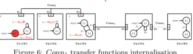
By applying the transformation to this connector, we ob-tain the model of Figure 6. Since the initial model con-tains just one writer, the connector topology remains in-tact, only its transfer functions and component behaviours are modified in that example. Functions U and D1 will
be integrated to CP 1 component. D2 (resp. D3) function
will be internalized in CP 2 (resp. CP 3). In each compo-nent, we export a new variable z (instead of x) in ports pi,
i∈ [1, 3]. For down functions ( D1, D2 and D3), we add
a C function in every transition labelled by port pi. This
function is of the form x = Di(z), i ∈ [1, 3].
Concern-ing U p function, a state and a transition are added before each transition labelled by the writing port p1 in the
com-ponent T 1− CP 1. The new transition executes a C func-tion of the form z = U (x). The new connector Conn0
1have
the following transfer functions: U p : xConn0
1 = zp1 and Down : zp1= zp2= zp3= xConn0 1. L1 L1’ start p1 z = U(x) x = D1(z) L1 start p2 x = D2(z) start L1 L2 p3 p4 x = D3(z) L1 start L2 p6 p5 L1 start L2 p7 T1-CP1 T2-CP2 T3-CP3 T4-CP4 T4-CP5 Conn0 1 Conn2 Conn3 p1 z x p2 z x p3 z x p4 x p5x xp6 p7x
Figure 6: Conn1transfer functions internalisation
4. DISCUSSION & CONCLUSION
BIP connectors, can be transformed into TT interfaces by successive application of two types of source-to-source transformations; Transfer functions internalisation and n + 1-ary connector to TT interface transformation. The first simplifies the connector transfer functions by mod-ifying components automata while keeping the same general behaviour of the model. The second transforms connector with simple transfer functions to TT interfaces.
The major asset of these source-to-source transformations, is that we don’t add new components requiring adding new tasks, a part from TT interfaces. These transformations focus on transforming atomic components by adding new ports, new variables and extending automata with new states and transitions. The number of added states strongly de-pends on the number of writers in the model and the number of transitions labeled by the port involved in the interaction. For that we propose in our future work to study differ-ent cases and to decide whether to modify compondiffer-ents au-tomata or add a task that orchestrates all interactions with-out altering components’ automata. Then, based on system constraints, a trade-off can be defined.
5. REFERENCES
[1] BIP2 Documentation, July 2012.
[2] T. Abdellatif, J. Combaz, and J. Sifakis. Model-based implementation of real-time applications. pages 229–238, May 2010.
[3] A. Basu, P. Bidinger, M. Bozga, and J. Sifakis. Distributed semantics and implementation for systems with interaction and priority. In Formal Techniques for Networked and Distributed Systems–FORTE 2008, pages 116–133. Springer, 2008.
[4] P. Bourgos. Rigorous design flow for program-ming manycore platforms.
[5] M. Bozga, M. Jaber, and J. Sifakis. Source-to-source architecture transformation for performance optimization in bip. Industrial Informatics, IEEE Transactions on, 6(4):708–718, 2010.
[6] H. Kopetz. The time-triggered approach to real-time system design. Predictably Dependable Computing Systems. Springer, 1995.
[7] H. Kopetz. The time-triggered model of computation. In Real-Time Systems Symposium, 1998. Proceedings., The 19th IEEE, pages 168–177. IEEE, 1998.
[8] K. D. Nguyen, P. Thiagarajan, and W.-F. Wong. A uml-based design framework for time-triggered applications. In Real-Time Systems Symposium, 2007. RTSS 2007. 28th IEEE International, pages 39–48. IEEE, 2007.