HAL Id: hal-01494509
https://hal.archives-ouvertes.fr/hal-01494509
Submitted on 23 Mar 2017
HAL is a multi-disciplinary open access
archive for the deposit and dissemination of
sci-entific research documents, whether they are
pub-lished or not. The documents may come from
teaching and research institutions in France or
L’archive ouverte pluridisciplinaire HAL, est
destinée au dépôt et à la diffusion de documents
scientifiques de niveau recherche, publiés ou non,
émanant des établissements d’enseignement et de
recherche français ou étrangers, des laboratoires
Volatility Strategies for Global and Country Specific
European Investors
Marie Brière, Jean-David Fermanian, Hassan Malongo, Ombretta Signori
To cite this version:
Marie Brière, Jean-David Fermanian, Hassan Malongo, Ombretta Signori. Volatility Strategies for
Global and Country Specific European Investors. Bankers Markets & Investors : an academic &
professional review, Groupe Banque, 2012, pp.17-30. �hal-01494509�
Volatility Strategies for Global and Country Specific European Investors
Marie Bri`ere1,3
Amundi Asset Management, France.
Universit´e Libre de Bruxelles, SBS-EM, Centre Emile Bernheim, Belgium.
Email : marie.briere@amundi.com
Jean-David Fermanian2,4
Universit´e de Paris-Dauphine, Ceremade, France.
Centre de Recherche en ´Economie et Statistiques (CREST), France.
Email : jean-david.fermanian@ensae.fr
Hassan Malongo2,3 Amundi Asset Management, France.
Universit´e de Paris-Dauphine, Ceremade, France.
Email : hassan.malongo@amundi.com
Ombretta Signori5
AXA Investments Managers, France.
Email : ombretta.signori@axa-im.com
This Version : 17 october, 2010
1Universit´e Libre de Bruxelles, Centre Emile Bernheim - Solvay Business School, Av. F.D. Rooselvelt, 50, CP 145/1, 1050 Brussels, Belgium.
2Universit´e de Paris-Dauphine, Centre de Recherche en Math´ematiques de la D´ecision (Ceremade), Place du Mar´echal De Lattre De Tassigny, 75775 Paris, France.
3Amundi Asset Management, 90 Boulevard Pasteur, 75015 Paris, France.
4Centre de Recherche en ´Economie et Statistiques (CREST), 15 Boulevard Gabriel Peri, 92245 Malakoff, France.
5AXA Investment Managers, 100 Esplanade du G´en´eral de Gaulle, 92932 Paris, France.
Abstract
Adding volatility exposure to an equity portfolio offers interesting opportunities for long-term investors. This
article discusses the advantages of adding a long volatility strategy for a protection to a global European equity
portfolio and to specific equity portfolios based in “core” or “peripheral” countries within the euro zone. A
European investor today has the choice of investing in US or European equity volatility. We check whether a
long volatility strategy based on VSTOXX futures is better than a strategy based on VIX futures. The benefit of
using volatility strategies as a hedge for equities is shown through a Mean/Modified-CVaR portfolio optimization.
We find that long volatility strategies offer valuable protection to all European equity investors. A long volatility
strategy based on VSTOXX futures offers better protection than a similar one based on VIX futures. It reduces
the risk of an equity portfolio more significantly, while providing more attractive returns. For specific European
investors, and despite major differences in local European equity markets, our long volatility strategy shows a
certain homogeneity and provides efficient protection, whatever the country.
Keywords : Investment strategy, Portfolio choice, Conditional Value-at-Risk, Implied volatility, Hedging.
JEL codes : G11, G15, G17
1
INTRODUCTION
Since the financial crisis in 2008-2010, many investors have shown greater interest in volatility strategies
be-cause of their attractive characteristics. Volatility tends to spike in times of market stress, and its movements are
known to be negatively correlated with risky asset returns. The US subprime crisis of 2008 or the recent European
sovereign debt crisis of 2010 are particularly good examples of this phenomenon (see Figure 1 in Appendix II).
Accordingly, adding volatility exposure to an equity portfolio can offer interesting opportunities for long-term
investors. This has been well documented in the academic literature. Daigler and Rossi (2006) show that the
strong negative correlation between the S&P 500 index and the VIX (implied volatility index of the S&P 500)
offers significant diversification benefits. Dash and Moran (2005) explore the relationship between the VIX and
hedge fund returns. They show that being long implied volatility is an excellent hedge against the risks of
port-folios that contain alternative-type investments. Bri`ere et al. (2010) examine the advantage of incorporating two
volatility strategies into an equity portfolio for long-term investors. They use a long volatility strategy with time
varying exposure that protects against equity risk and a short variance swap strategy that reduces the overall
cost of the long volatility strategy and which is partially hedged by the long volatility strategy in times of crises.
Taken separately, each of the strategies shifts the efficient frontier significantly outward, but combining the two
produces even better results.
One of the simplest ways to get exposure to volatility is to invest in implied volatility futures such as VIX or
VSTOXX futures. VIX futures are based on the 30-day implied volatility deduced from S&P 500 traded options
and were introduced on the CBOE in March 2004. VSTOXX futures are the equivalent1of VIX futures in Europe and are based on EuroStoxx 50 options. They were introduced on the Eurex exchange market in September 20052.
1. VDAX, VCAC or VSMI are other implied volatility indices on respectively German, French and Swiss equity indices, but futures on these indices are not listed yet.
2. These futures are listed with monthly expiries which are usually on the Wednesday prior the second to last Friday of their respective expiration/maturity month.
While the situation of US investors has been extensively investigated, this is not the case in Europe. At
present, such an investor has the choice between two types of strategies : one based on VSTOXX futures that
appears as the most logical hedge for his European equity risk but which is relatively less liquid than the US
equivalent strategy based on VIX, or the alternative VIX futures strategy. As most of the work on this topic has
been done for US investors in the academic literature, we reconsider the problem from the viewpoint of European
investors facing this choice. We first analyze the relationship between a global European equity index and long
volatility strategies based on VIX and VSTOXX futures. Next, we check whether these strategies provide a way
to hedge European country equity risk exposures. Specific country equity markets are represented by a selection
of core European countries (France and Germany) and peripheral countries (Portugal, Ireland, Greece and Spain)
which are currently experiencing economic difficulties (high unemployment and budget deficits, high risk on their
sovereign debt). The “country per country” analysis is interesting in itself, beside obvious practical implications.
Indeed, it is a way of checking the robustness of a long volatility strategy as a hedge against equity exposures,
when the strategy is related to the Euro (or US)-zone globally and the exposure is purely national. Our results
show that it is not clear whether the choice between VSTOXX and VIX futures is definitive, independently of
the specification of each national equity market. In fact, some disparities may exist across the European equity
markets themselves. And even if the correlation between US and EU equity indices is high, indices in implied
volatility like VSTOXX and VIX highlight the equity risks for two different regions which rely partly on different
specific drivers. We finish the study by giving the benefit of using this kind of volatility strategy through a
Mean/Modified-CVaR portfolio optimization for both the global and the specific European investor.
We believe this research is original for two reasons. First, unlike most previous research (e.g. Dash and Moran
(2005) or Daigler and Rossi (2006)), we propose a long volatility strategy which uses real future prices data and
thus takes explicitly into account the cost (or the gain) of rolling these futures positions. Actually, in the academic
without calculating the rolling cost (or gain) associated with these futures when they evaluate their volatility
strategies. In this article, we build a long volatility strategy which is more realistic and we examine the advantage
of incorporating it into an equity portfolio. Second, since the returns of volatility strategies are asymmetric and
leptokurtic, we propose an appropriate optimization technique through a measure of risk which captures higher
order moments. In fact, most of the previous studies in the literature use mean-variance optimization even if
there is empirical evidence that financial asset returns are not normally distributed (e.g. Andersen et al. (2000),
Goetzmann et al. (2002)). Investors who are sensitive to extreme events of return distributions should not use
mean-variance optimization because by ignoring the underlying skewness and kurtosis, this technique allocates
the assets sub-optimally (Leland (1999), Cremers et al. (2005)). In this paper, our reference measure of risk is
a Conditional ”Modified” Value-at-Risk (CVaR) proposed by Cao et al. (2010). We use this semi-parametric
measure of risk because it provides a good picture of tail risks, especially under strongly adverse conditions.
We find that long volatility strategies offer valuable protection to European equity investors. A long volatility
strategy based on VSTOXX futures offers better protection than the addition of a long volatility strategy based
on VIX futures for a global European investor. To be specific, a long volatility VSTOXX strategy offers a way
of reducing more than half of the modified CVaR of the equity-only portfolio of a global European investor, and
the returns are more attractive than when using the VIX strategy. This is explained by the fact that rolling
VSTOXX futures is much less costly than rolling VIX futures, as the volatility term structure tends to be steeper
for VIX than for VSTOXX futures. For all specific European investors, our volatility hedging strategy has shown
a certain homogeneity. Our findings show that adding futures on implied volatility to a specific equity portfolio
provides results close to those obtained with a global European equity portfolio, at least qualitatively. In
particu-lar, we find that specific equity portfolios with VSTOXX futures are generally better than those with VIX futures.
The paper is organized as follows. In section 2, we detail the methodology used to build the volatility strategy
the descriptive statistics. Section 4 is related to the empirical results of optimal portfolios for a global European
investor and for specific country investors. Section 5 summarizes our conclusions and outlines the implications
for further research.
2
METHODOLOGY
Long exposure to volatility
We consider a European equity investor willing to take systematic exposure to volatility in his equity portfolio.
From a practical point of view, this investor can hedge his equity risk by using volatility options or rolling futures
on implied volatility. As in Bri`ere et al. (2010), we build a volatility strategy which tries to take advantage of
the mean-reverting property of volatility and which rolls a long position in futures. Our long volatility strategy
consists in rolling monthly the third3 nearest futures contract (compared to the last day of the current month). Broadly, the investment consists in putting a portion of the investor’s capital in cash (which is used for the futures
margin deposits) and another portion in a specified number of VSTOXX or VIX futures such that the impact
of a 1-point variation in the prices of the futures is equal to F1
t−1 ∗ 100% (where Ft−1 is the price of the future
at time t-1). As the three-month VIX and VSTOXX futures prices are available only since February 2007, we
have estimated their prices before this date by estimating the average linear relation between futures prices and
their respective index during their period of existence. These estimated values of this linear model provide the
futures prices before their period of existence4. Moreover, when we constructed the volatility strategy, we took into account the cost (or the gain)5of rolling these futures. As we want to use the volatility strategy as an equity
3. Actually, several futures contract maturities are possible (one month, two months etc). In general, we seek a hedge against equity index movements in the short run through volatility exposure. Thus, the shorter the maturity of the futures, the better our hedge should perform. In fact, this is not the case. Indeed, rolling one-month or two-month futures at the end of each month generates negative returns for a similar level of risk. Conversely, three-month futures seem to provide a good balance between relevance (time-horizon of the underlying) and smoothness.
4. The R2 of the linear regression between the three-month VIX futures and VIX index over the period from February 2007 to
December 2010 is equal to 0.78 while it is equal to 0.75 for the regression with the three-month VSTOXX futures over the period from February 2007 to December 2010.
5. The cost (or gain) of rolling the three-month VIX and VSTOXX futures prior to their respective period of existence is taken equal to the average cost (or gain) to roll these futures during their period of existence.
hedge and exploit the negative correlation between implied volatility and equity returns, we have normalized the
volatility exposure by setting its monthly 95% modified CVaR at the same targeted level of risk as the equity
reference asset class. Implicitly, it means that we want the worst scenarios for the index to be the best ones for
the volatility strategy, broadly speaking. Once calibrated, we have written the return of the volatility strategy
as the risk-free return plus a fixed proportion (also called degree of leverage) of the capital in VSTOXX or VIX
futures (see Bri`ere et al. (2010) for more details on the strategy). The returns of the long volatility strategies
between t and t + 1 are then calculated as follows :
rLVt+1= rft+1+ θ ∗ P &LF utures (1)
P &LF utures= 1
Ft(Ft+1− Ft) (2)
where rft is the cash return and Ft6 is the price of the future at time t. θ is the so-called degree of leverage, chosen so that the modified CVaR of the long volatility strategy is the same as the modified CVaR of the equity
portfolio. The detailed methodology used to calibrate θ is given in Appendix I.
Risk measure
When asset returns are not normally distributed, their variance is no longer an appropriate measure of risk.
To be more specific, variance often leads to an underestimation or a biased view of the true underlying risks since
asset returns are generally both skewed and leptokurtic. Even if there is empirical evidence that financial asset
returns are not normally distributed, one of the most commonly used measures of risk in the financial industry is
Value-at-Risk7(VaR) based on the standard normal distribution. Its success is largely due to its equivalence with the standard deviation in the case of underlying Gaussian distributions (see Jorion (2007) e.g.). As an alternative
6. The investor should consider that the contract value for VSTOXX futures is EUR 100 per index point of the underlying while it is$1000 per index point of the underlying for VIX futures. As the amount to invest in the long volatility strategy evolves with time, the investor will invest each month in a number of futures equal to Nt∗θ
M ∗Ft where Nt is the part of the investor’s capital allocated to
the volatility strategy (cash + futures position) at date t and M = 100 if he/she invests in VSTOXX futures or M = 1000 if he/she invests in VIX futures.
to dealing with non-normally distributed assets, Favre and Galeano (2002) have proposed a new measure of
risk called “modified Value-at-Risk ”. This risk measure takes into account higher-order moments and replaces
the quantile of the standard normal distribution with a modified quantile approximated by the Cornish-Fisher
expansion8 (see e.g. Ord and Stuart (1999)). Modified VaR is defined by :
Mod V aR(1 − α) = −[µ + σ ∗ Q(α)] Q(α) = zα+1 6(z 2 α− 1) ∗ S + 1 24(z 3 α− 3zα) ∗ (K − 3) − 1 36(2z 3 α− 5zα) ∗ S 2 ,
where µ, σ, S and K denote the mean, the standard deviation, the skewness and the kurtosis of the portfolio’s
returns respectively. Obviously, zαdenotes the α-quantile of the standard normal distribution N (0, 1).
Another way to measure the risk of a portfolio is to invoke Conditional Value-at-Risk (CVaR), as introduced
by Rockafellar and Uryasev (2000). It is defined as the average of the loss quantiles exceeding the VaR at the
threshold α, but rescaled by 1 − α. In the case of continuous underlying distributions, as in our framework, CVaR
is equal formally to the Expected Shortfall (also called Tail Conditional Expectation)9: see Tasche (2002). Since CVaR is a so-called “coherent measure of risk”, in the sense of Artzner et al. (1999), it has become a standard
in risk management. In this article, however, our reference measure of risk will be Conditional Value-at-Risk
(CVaR) based on a “modified Value-at-Risk ”. This measure is a semi-parametric approach proposed by Cao et al.
(2010), who introduce it to hedge different long positions in equity indices with index futures contracts. We have
chosen modified CVaR instead of modified VaR because the latter risk measure still suffers from some well-known
“drawbacks” of a VaR measure. Most of these are well documented in the literature (see Danielsson (2002), e.g.).
For instance, instability is greater for VaR (modified or not) than for CVaR (modified or not) when dealing with
very high/small levels of α, and particularly when the return distributions are strongly non normal (Boudt et
8. The higher-order moments taken into account in the modified VaR formula are skewness and kurtosis. Some authors have considered more “correction” terms in the Cornish-Fisher expansions and have found that increasing the order does not necessarily improve the approximation (see e.g. Jaschke (2002)).
al. (2007)). Moreover, beside its property of coherence, CVaR is superior to VaR in optimization applications
(Rockafellar and Uryasev (2000)) and has nicer mathematical properties10 than VaR. In practice, VaR is less than CVaR with the same confidence level, and a risk-averse investor may prefer CVaR because it copes with
large losses when they occur. From an analytic point of view, the modified CVaR is written as :
Mod CV aR(1 − α) = 1 α Z 1 1−α Mod V aR(x) dx = −[µ + σ α Z 1 1−α Q(1 − x)dx].
Being simple to implement, this expression can be rewritten (Cao et al. (2010)) as
Mod CV aR(1 − α) = −µ − σ ∗ [M1+ 1 6(M2− 1) ∗ S + 1 24(M3− 3M1) ∗ K − 1 36(2M3− 5M1) ∗ S 2], where Mi= α1Rzα −∞x
if (x)dx and where f (.) is the standard normal probability density function.
3
THE DATA
The study covers the period between January 1999 and December 2010. We use the MSCI EMU index in total
return terms (performance includes reinvested dividend gains) for the global European equity index11. For the specific European equity indices, we rely on the MSCI France, Germany, Portugal, Ireland, Greece and Spain,
also in total return12. To build the long volatility strategy, our underlyings are the third next to expire VSTOXX and VIX futures contracts (three-month maturity at buying date). The risk-free rate for cash investment is the
one-month Euribor rate. As all the strategies are considered from the point of view of a European investor, we
have converted the US investment in VIX futures into euro. VSTOXX and VIX futures are provided by
Bloom-berg, all other series (equity and implied volatility indices, EUR/USD exchange rate and Euribor rate) come from
10. In financial applications, the CVaR of a portfolio is a continuous and convex function of the underlying portfolio positions whereas its VaR may be a discontinuous function (Pflug (2000)).
11. As of December 2010, the MSCI EMU contains 267 stocks which represent 11 country indices within the European Monetary Union at December 31, 2010 : Austria (1.06%), Belgium (3.04%), Finland (3.42%), France (32.71%), Germany (28.35%), Greece (0.75%), Ireland (0.82%), Italy (9.27%), the Netherlands (8.40%), Portugal (0.88%), and Spain (11.30%). Full details are available at www.msci.com.
12. MSCI France, Germany, Portugal, Ireland, Greece and Spain contain respectively 75, 52, 8, 4, 8 and 26 stocks in December 2010.
Datastream. Monthly closing prices are used for the equity indices, the VSTOXX and VIX indices, the risk-free
rates, the exchange rates and the corresponding monthly settlement prices of the futures contracts.
Table 1 (Appendix III) provides descriptive statistics for the MSCI-EMU index and the two long volatility
strategies over the period February 1999 and December 2010. In terms of annualized returns, the long volatility
strategy based on VSTOXX futures (LV-VSTOXX) appears to be the most attractive, followed by the long
vola-tility strategy based on VIX futures (LV-VIX) and the equity index (4.50%, 2.84% and 1.76% respectively). The
substantial difference in performances between the long volatility strategies based on VSTOXX and VIX futures
is explained by the fact that the former are less costly to roll than the latter13. To keep a volatility exposure month after month, the investor has to buy at month end the third to expire future and sell the one bought
the month before (which now becomes the second to expire), thus paying (or receiving) each month the spread
between the third and the second futures contracts. This induces a cost (or a gain) which can be substantial : the
rolling gain is 0.43% for VSTOXX futures, whereas it is costly (-1.16%) for VIX futures14. This explanation is highlighted by Figures 2 and 3 (Appendix II). The spread between the third and the second futures VIX contracts
is 61.7% of the time larger than the equivalent VSTOXX spread (Figure 2). Even if this spread decreases with
maturity (see Figure 3), it appears that it is always larger for VIX than for VSTOXX futures.
Modified CVaR has been calibrated15 to be identical for the volatility strategies and the equity exposure. However, volatility differs quite sharply. Whereas it is 19.45% for equities, it is much stronger for both volatility
strategies (33.89% and 30.76% for VSTOXX and VIX respectively). An analysis of higher-order moments shows
that the three assets’ distribution departs strongly from normality. While the skewness of the MSCI EMU is
negative (-0.38), confirming the high extreme risks of the equity exposure, it is strongly positive for both
vola-13. Note that the observed differences in performance between the two strategies are not due to exchange rates. We obtained very similar results when we considered the strategies’ performances in local currency terms.
14. If we did not take into account this rolling cost, the annualized return of the long volatility strategies would be much closer, 4.07% for VSTOXX vs 4.00% for VIX futures respectively.
tility strategies (1.39 and 1.66 for VSTOXX and VIX respectively). This confirms the attractive role that long
volatility strategies may play in an equity portfolio, providing valuable protection against the leftward
asymme-try of the equity exposure. The kurtosis of all three assets is greater than 3 (4.00, 7.27 and 10.60 for the equity
index, VSTOXX and VIX respectively) and the Jarque-Bera statistic rejects the null hypothesis of normality
for the three series at the 5% significance level. These results confirm the importance of taking into account the
higher-order moments when evaluating the risk.
Table 2 (Appendix III) provides the correlation matrix between the European equity index and the two
vo-latility strategies. We observe that the two vovo-latility strategies are strongly correlated (0.80). The correlation
coefficient between European equities and volatility strategies is -0.66 for VSTOXX while it is equal to -0.63 for
the VIX. This strong negative correlation confirms the role of volatility strategies as a partial hedge for the equity
exposure (Dash and Moran (2005), Daigler and Rossi (2006), Bri`ere et al. (2010)). However, even if VSTOXX
futures appear to have a slightly lower correlation with equities than do VIX futures, this difference is not
signi-ficant when we apply the Hotelling/Williams test16.
Table 3 (Appendix III) provides descriptive statistics for the equity indices of specific countries over the period
February 1999 to December 2010. The Spanish equity index has the highest annualized returns (4.08%) followed
by France and Germany (2.48% and 2.40% respectively). Ireland and Greece have the worst returns (-9.97%
and -7.16% respectively) and also the strongest volatility (23.10% and 29.33% respectively) and modified CVaR
(16.79% and 19.85% respectively) compared to the others indices (for example 13.77% for Portugal modified
CVaR and 12.21% for France). These results are hardly surprising considering the recent European crisis, which
has fuelled investors’ concerns about the economic situation of these two countries (budget deficit, sovereign debt
risk). Maximum drawdowns are also particularly high for both countries (-81.56% for Ireland and -76.43% for
Greece). The analysis of higher order moments of the return distribution clearly highlights that all country returns
16. The Hotelling/Williams test checks whether the correlation between Z and X differs from the correlation between Z and Y, where X, Y and Z are three variables measured on the same set of observational units.
are non normally distributed (negative skewness and excess kurtosis), a result confirmed by the Jarque-Bera test.
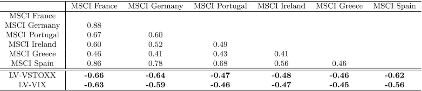
Table 4 (Appendix III) reports the correlation matrix between country equity returns and the two volatility
strategies. As expected, we observe a stronger correlation of stock indices between the “core” European countries,
namely France and Germany (0.88), than between the peripheral ones (around 0.5, for Portugal, Ireland, Greece
and Spain). The correlations between the country equity indices and the long volatility strategies based on
VSTOXX and VIX futures are strongly negative (between -0.45 and -0.66). These negative correlations are
greater with the core European countries than with the peripheral ones. Moreover, they are always higher with
VSTOXX futures than with VIX futures. In line with what we found for global European equity investment, we
observe that VSTOXX futures provide a slightly higher diversification benefit than VIX futures for each specific
European country investor, but the differences in correlations are not significant when the Hotelling/Williams
test is applied.
4
OPTIMAL PORTFOLIOS
In what follows, we examine the advantages for a European investor of adding a volatility strategy based
on VSTOXX or VIX futures. We first build optimal portfolios made of global European equities and volatility
strategies and then compare them with a pure equity investment. Next, we consider the case of specific European
investors who want to hedge their local equity exposure with volatility strategies. We check if these advantages
are unique whatever the specific characteristics of each equity market.
Optimal portfolio for a global European Investor
To determine the interest of adding a systematic exposure to volatility to a European equity portfolio and
compare VIX with VSTOXX futures investments, we consider two basic types of portfolios : Equity with a long
we compare them with the global European equity investment. Efficient frontiers made of VIX and
equity-VSTOXX (Figure 4 in Appendix II) are calculated by minimizing the Modified CVaR at threshold α = 95% for
different levels of expected returns. We provide global minimum CVaR portfolios compositions and performances
in Table 5 (Appendix III).
Allocating around 45% (45.47% for the VSTOXX strategy and 42.77% for the VIX) of the portfolio to the
long volatility strategies is necessary to achieve the minimum level of risk. The addition of long volatility
stra-tegies makes it possible to reduce more than half the modified CVaR of the equity-only portfolio (4.97% for the
equity-VSTOXX and 5.16% for the equity-VIX vs 13.14% for the equity-only portfolio). Moreover, both portfolios
have much more attractive returns (5.94% vs 4.72% ) than the equity-only portfolio (1.76%).
An analysis of extreme negative events shows that the maximum monthly loss is more than halved (-5.85%
and -8.61% ) when including VIX and VSTOXX strategies respectively, compared with the equity-only portfolio
(-17.53%). Furthermore, looking at the maximum drawdown, we observe that the equity-VSTOXX portfolio has
the smallest drawdown (-11.19%) compared to the equity-VIX portfolio (-25.72%) and the equity-only (-55.69%).
The portfolio’s skewness also becomes positive (1.30 and 0.67 when adding VSTOXX and VIX respectively), and
should be compared to the strong negative skewness of the equity-only investment (-0.38).
On the whole, our findings show that while both volatility strategies are attractive for hedging a strategic
equity exposure, a long volatility strategy based on VSTOXX futures offers better protection for a European
equity investor than a similar strategy based on VIX futures. Not only are extreme risks smaller, but the returns
of the portfolio are also substantially higher. This is true not only for the minimum 95% modified CVaR but also
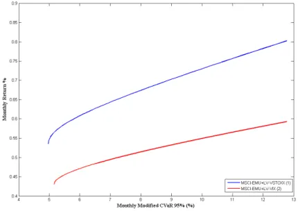
for most levels of risk17. This result is highlighted by Figure 4 (Appendix II), which gives the efficient frontiers for the MSCI-EMU index with long volatility strategies. We clearly observe that the efficient frontier of the equity
portfolio with VSTOXX futures is always above the efficient frontier of the equity portfolio with VIX futures and
we see that this gap increases with the risk level of the strategy.
Optimal portfolios for specific European investors
Tables 6 and 7 (Appendix III) give the optimal weights and performances of the portfolios with VSTOXX
and VIX futures (respectively) for the six specific country investors. By and large, for all country investors, our
findings are consistent with what we found in the previous section. Adding around 45% (between 36.40% and
46.14%) of a volatility strategy based on VSTOXX or VIX futures to a European equity portfolio greatly improves
the risk-adjusted returns of the portfolios. The equity-VSTOXX portfolios have much higher annualized returns
than the equity-VIX portfolios for all country investors. In some cases (Greece and Ireland), adding a VSTOXX
strategy makes the portfolio’s performances positive (1.07% and 0.01% respectively), whereas the inclusion of VIX
strategies is not sufficient to counterbalance the strong negative performances of these equity markets (-7.16%
and -9.97% respectively over the period).
As in the case of the global European investor, we observe that adding volatility exposure strongly reduces
the risks of the equity-only portfolios. For example, the 95% modified CVaR of the German equity portfolio
is equal to 16.06% (see Table 3, Appendix III) compared with 6.17% and 6.51% when we add long volatility
based on VSTOXX and VIX futures respectively. Moreover, for all specific European investors, the addition of a
long volatility strategy to an equity portfolio is an interesting way to reduce the maximum losses and maximum
drawdown, without significantly diminishing the maximum monthly gain. For instance, for an Irish equity
inves-tor, the maximum drawdown (-81.56%) is reduced to -45.54% and -40.46% when a volatility strategy with VIX
and VSTOXX (respectively) is added, whereas the maximum gain is actually increased from 14.15% to 21.80%.
Finally, our results show that, on the whole, a long volatility investment in VSTOXX futures is a better hedge
than VIX futures for all specific investors. Not only are returns significantly higher, but the portfolios also exhibit
Our hedging strategy with volatility futures has shown a remarkable homogeneity even though there may be
disparities between European equity markets. Actually, country equity indices differ in terms of sector composition
(Cooper and Kaplanis (1994), Tesar and Werner (1995)) and as economic difficulties are regional in nature,
national markets respond differently to global shocks (Rouwenhorst (1998)). These disparities are reflected in the
fact that European equity markets are not particularly highly correlated18. On the whole, for both the core EU economies (France and Germany) and the peripheral countries (Portugal, Ireland, Greece and Spain), we find
that a long volatility strategy based on VSTOXX futures provides a good way to hedge local equity exposures. In
fact, it is better than a similar VIX futures exposure. These results confirm that, compared with VIX, VSTOXX
better reflects the financial risks19 in Europe.
5
CONCLUSION
Since the recent financial crisis, the need to find strategies for hedging exposures to risky assets, especially
equities, has aroused a great deal of interest among long-term investors, and the appeal of volatility strategies
has increased considerably. If the case of US investors has been extensively studied, the particular situation of
European investors has not received much attention. This paper tries to fill the gap by investigating the interest
of adding volatility exposure to a European equity portfolio, whether global or on a specific country index. In
the context of the recent European crisis, we believe this research may be of practical value for many investors.
By and large, our results confirm the interest of adding volatility exposure (based on VSTOXX or VIX futures)
to a European equity portfolio. We show that a long volatility strategy based on VSTOXX futures offers better
18. Only Germany, France and Spain show a high correlation over the studied period (see Table 4, Appendix III).
19. For instance, when Fitch rating agency downgraded Greece’s government debt to BBB+ from A- with a negative outlook at December 8, 2009, the EuroStoxx 50 index fell of -2.70% whereas VSTOXX and VIX index increased of 13.81% and 2.53% respectively between December 7 and December 9, 2009. The impact of this news reflected by the spike of VSTOXX index, had affected more the European market than the US market.
protection than a long volatility strategy based on VIX futures when dealing with a European equity investment,
whether global or specific to a euro zone country. This result is explained by the fact that the steepness of the
curve for VIX futures incurs a higher cost of carry compared with that for VSTOXX futures. In addition, as
VSTOXX and VIX index price the risk in different regions with specifics drivers, the fall in the European equity
index will be higher than that in the US equity index during a European crisis for instance. VSTOXX futures
are then better candidates than VIX futures to hedge the European equity risk.
One of the limitations of our work relates to the period of time needed to roll the futures. Although the period
from 1999 to 2010 contains some major economic and financial crises, we cannot be sure that, in future, there
will be no volatility movements that induce high rolling costs and could impair the performances of the proposed
hedge. Having a systematic long exposure in futures on implied volatility is still a sophisticated investment
strategy that can produce substantial losses if not managed appropriately, according to the phases of the stock
market. One interesting continuation of this work would be to build a tactical strategy based on specific signals
and making it possible to refine the volatility exposure and buy an optimal number of futures on implied volatility,
References
[1] Andersen J.V., Simonetti P. and Sornette D. (2000). Portfolio Theory for Fat Tails. International Journal of
Theoretical and Applied Finance 3(3):523-535.
[2] Artzner P., Delbaen F., Eber J.M. and Heath D. (1999). Coherent Measures of Risk. Mathematical Finance
9(3):203-228.
[3] Boudt K., Croux C. and Peterson B.G. (2007). Estimation and decomposition of downside risk for portfolios
with non-normal returns. MPRA Paper. University Library of Munich.
[4] Bri`ere M., Burgues A. and Signori O. (2010). Volatility Exposure for Strategic Asset Allocation. The Journal
of Portfolio Management 36(3):105-116.
[5] Cao Z., Harris R.D.F. and Shen J. (2010). Hedging and Value at Risk: A Semi-Parametric Approach. Journal
of Futures Markets 30(8):780-794.
[6] Cooper I. and Kaplanis E. (1994). Home Bias in Equity Portfolios, Inflation Hedging, and Intemational Capital
Market Equilibrium. Review of Financial Studies 7(1):45-60.
[7] Cremers J.H., Kritzman M. and Page S. (2005). Optimal Hedge Fund Allocations. The Journal of Portfolio
Management 31(3):70-81.
[8] Daigler R.T. and Rossi L. (2006). A Portfolio of Stocks and Volatility. The Journal of Investing 15(2):99-106.
[9] Danielsson J. (2002). The emperor has no clothes: Limits to risk modelling. Journal of Banking & Finance
26(7):1273-1296.
[10] Dash S. and Moran M.T. (2005). VIX as a Companion for Hedge Fund Portfolios. The Journal of Alternative
Investments 8(3):75-80.
[11] Favre L. and Galeano J.A, (2002). Mean-modified Value at Risk Optimization With Hedge Funds. The
Journal of Alternative Investment 5(2):21-25.
[12] Goetzmann W., Ingersoll J., Spiegel M. and Welch I. (2002). Sharpening Sharpe Ratios. NBER Working
Paper No. 9116.
[13] Jaschke S.R. (2002). The Cornish-Fisher expansion in the context of deltagamma- normal approximations.
Journal of Risk 4(4):33-52.
[14] Jorion P. (2007). Value At Risk. 3rd Ed., McGraw Hill.
[15] Leland H., (1999). Beyond mean-variance: risk and performance measures for portfolios with nonsymetric
[16] Ord K. and Stuart A. (1999). Kendall’s Advanced Theory of Statistics, Volume 1 : Distribution Theory, 6th
edition. Oxford University Press.
[17] Pflug G.C. (2000). Some remarks on the value-at-risk and the conditional value-at-risk, in Uryasev S.P. (ed),
Probabilistic Constrainted Optimization: Methodology and Applications. Kluwer, Norwell, MA, 278-287.
[18] Rockafellar R.T. and Uryasev S.P. (2000). Optimization of conditional value-at-risk. Journal of Risk
2(3):21-42.
[19] Rouwenhorst K.G. (1999). European Equity Markets and EMU: Are the Differences Between Countries
Slowly Disappearing? Financial Analysts Journal 55(3):57-64.
[20] Tasche D. (2002). Expected Shortfall and Beyond. Journal of Banking & Finance 26(7):1519-1533.
[21] Tesar L.L. and Werner I.M. (1995). Home Bias and High Turnover. Journal of International Money and
Appendices
Appendix I
From a practical standpoint, we specify here the way the parameter θ is calibrated, as well as the optimization
procedure we used to obtain the optimal portfolios. Let us denote
– rft the (monthly) short rate, – Ft the spot level of the future,
– It the spot level of the equity index,
– PLV
t the t-value of the LV strategy, – PG
t the t-value of the global strategy, mixing a certain amount of the index and of the LV strategy, – PtF is the market value of a future at t,
– NLV
t the amount of cash that will be invested in the LV strategy at t, – M the reference notional of a VIX (or VSTOXX) future,
– mtthe number of futures contracts the investor will buy at t and sell at t + 1.
At t = 0, N0LV are invested in cash and the investor has entered into m0 futures. We have then
P0LV = N0LV = N0LV ∗ 1 + m0∗ P0F with P0F = 0.
At t = 1, we have
P1LV = N0LV(1 + rf1) + m0P1F = N0LV(1 + rf1) + m0(F1− F0)M.
The P&L between t = 0 and t = 1 is then
∆PLV
0 = P1LV − P0LV = N0LVr f
1+ m0(F1− F0)M. The associated return is
∆PLV
0 /P0LV = r f
1+ m0(F1− F0)M/N0LV. Similarly, the P&L generated between t and t + 1 is
∆PLV
t = Pt+1LV − PtLV = NtLVr f
t+1+ mt(Ft+1− Ft)M, where NLV
t is the cash amount that is available at t. Here, since we sell the whole portfolio at the end of every month, PLV
∆PLV
t /PtLV = r f
t+1+ mt(Ft+1− Ft)M/NtLV. The return of the long volatility strategy between t and t + 1 is given by
rt+1LV = ∆PtLV/PtLV = rft+1+ νt· ∆Ft/Ft,
νt:= FtmtM/NtLV·
We make the assumption that νtwill be a constant θ. As we want the level of risk of the long volatility strategy
to equal the level of risk of the equity only portfolio, we calibrate θ by the equation
M od CV aRα(∆PtLV/PtLV) = M od CV aRα(∆It/It).
Thus, we get the estimate ˆθ. The constancy of θ means that mt' Cst/Ft. Thus, the number of futures we buy is inversely proportional to the spot level of the future. This pattern of the strategy makes it possible to profit
from the mean reverting properties of volatility : the investor’s exposure is increased when volatility is low, it is
decreased when volatility is high (Bri`ere et al. (2010)). Moreover, before building the optimized portfolios, we
have assumed that the index strategy is static in the sense that we do not use cash regularly to buy/sell additional
amounts of the equity index. Our optimization procedure consists in finding a parameter β ∈ [0, 1] that is the
percentage of cash which will be invested in the equity index at the initial date. Such a parameter β minimizes
the 95% modified CVaR of the global strategy. Our optimization problem is then
ˆ
β = arg minβCV aRα(∆PtT/PtT).
With the same methodology as above, the returns of the global strategy between t and t + 1 are now
∆PtG/PtG = β · ∆It/It+ (1 − β) · ∆PtLV/PtLV.
Appendix II
Figure 1 – Daily closing prices on the EuroStoxx 50, VSTOXX and VIX index
This figure displays monthly closing prices on the EuroStoxx 50, VSTOXX and VIX index over the period February 1999-December 2010.
Figure 2 – Spread between the third and the second month futures
This figure displays the monthly spread (in % volatility) between the third and the second futures prices of VSTOXX and VIX over the period February 2007-December 2010.
Figure 3 – Average volatility term structure
This figure displays the average price of the first, second and third futures contracts for VSTOXX and VIX over the period February 2007-December 2010.
Figure 4 – Efficient Frontiers for global European investor
This figure displays the efficient frontiers of MSCI-EMU with VSTOXX (1) and MSCI-EMU with VIX (2) over the period February 1999-December 2010.
Appendix III
Table 1 – Descriptive Statistics for MSCI EMU index and long volatility strategies
This table reports the descriptive statistics for the MSCI EMU index and the long volatility strategies based on VSTOXX and VIX futures over the period February 1999-December 2010.
MSCI-EMU LV-VSTOXX LV-VIX Ann. Geo. Mean 1.76% 4.50% 2.84%
Ann. Std. Dev. 19.45% 33.89% 30.76% Max Monthly Loss -17.53% -19.68% -16.98% Max Monthly Gain 16.18% 48.26% 53.67%
Max Drawdown* -55.69% -47.98% -49.79% Skewness -0.38 1.39 1.66
Kurtosis 4.00 7.27 10.60 Mod. CVaR (95%)** 13.14% 13.14% 13.14% Jarque-Bera Stat (95%)*** 9.31 154.50 410.21
* The maximum drawdown is defined as the largest drop of a given asset within the sample period. ** VSTOXX and VIX strategies have been calibrated with a parameter θ respectively equal to 0.63 and 0.70.
*** The Jarque-Bera statistic is χ2(2) distributed under the null hypothesis of normality of residuals.
Table 2 – Correlation matrix between MSCI EMU index and long volatility strategies
This table gives the correlation matrix between the MSCI EMU index and the long volatility strategies based on VSTOXX and VIX futures over the period February 1999-December 2010.
MSCI-EMU LV-VSTOXX LV-VIX MSCI-EMU
LV-VSTOXX -0.66
Table 3 – Descriptive statistics for specific countries equity indices
This table gives the descriptive statistics of specific country equity indices over the period February 1999-December 2010.
MSCI France MSCI Germany MSCI Portugal MSCI Ireland MSCI Greece MSCI Spain
Ann. Geo. Mean 2.48% 2.40% -0.62% -9.97% -7.16% 4.08%
Ann. Std. Dev. 18.71% 23.09% 18.89% 23.10% 29.33% 20.84%
Max Monthly Loss -15.98% -24.93% -19.97% -22.49% -29.88% -17.22%
Max Monthly Gain 13.55% 20.94% 13.37% 14.15% 24.90% 16.68%
Max Drawdown* -58.14% -67.91% -57.03% -81.56% -76.42% -49.59%
Skewness -0.38 -0.35 -0.56 -0.73 -0.21 -0.31
Kurtosis 3.54 4.61 4.60 3.50 3.92 3.92
Mod. CVaR (95%) 12.21% 16.06% 13.77% 16.79% 19.85% 13.66%
Jarque-Bera Stat(95%)** 5.11 18.36 22.78 14.09 6.13 7.29
* The maximum drawdown is defined as the largest drop of a given asset within the sample period. ** The Jarque-Bera statistic is χ2(2) distributed under the null hypothesis of normality of residuals.
Table 4 – Correlation matrix between Country equity indices and long volatility strategies
This table reports the correlation matrix between the country equity indices and the long volatility strategies based on VSTOXX and VIX futures over the period February 1999-December 2010.
MSCI France MSCI Germany MSCI Portugal MSCI Ireland MSCI Greece MSCI Spain MSCI France MSCI Germany 0.88 MSCI Portugal 0.67 0.60 MSCI Ireland 0.60 0.52 0.49 MSCI Greece 0.46 0.41 0.43 0.41 MSCI Spain 0.86 0.78 0.68 0.56 0.46 LV-VSTOXX -0.66 -0.64 -0.47 -0.48 -0.46 -0.62 LV-VIX -0.63 -0.59 -0.46 -0.47 -0.45 -0.56
Table 5 – Optimal portfolio allocations for global European investors
This table reports the optimal compositions and performances of the portfolios that minimize the 95% modified CVaR for MSCI EMU index and long volatility strategies (VIX and VSTOXX) over the period February 1999-December 2010.
MSCI-EMU + LV-VSTOXX MSCI-EMU + LV-VIX Ann. Geo. Mean 5.94% 4.72%
Ann. Std. Dev. 11.55% 10.58% Max Monthly Loss -8.61% -5.85% Max Monthly Gain 15.45% 13.96% Max Drawdown* -11.19% -25.72% Skewness 1.30 0.67 Kurtosis 8.10 4.72 Mod. CVaR (95%) 4.97% 5.16% MSCI-EMU 54.53% 57.23% LV-VSTOXX 45.47% -LV-VIX - 42.77%
Table 6 – Optimal portfolio allocations for specific European country investors with VSTOXX This table reports the optimal compositions and performances of the portfolios that minimize the 95% modified CVaR for MSCI country indices and VSTOXX over the period February 1999-December 2010.
MSCI France MSCI Germany MSCI Portugal MSCI Ireland MSCI Greece MSCI Spain
+LV-VSTOXX +LV-VSTOXX +LV-VSTOXX +LV-VSTOXX +LV-VSTOXX +LV-VSTOXX
Ann. Geo. Mean 5.94% 7.10% 3.89% 0.01% 1.07% 7.34%
Ann. Std. Dev. 11.55% 14.34% 13.22% 18.59% 19.19% 11.96%
Max Monthly Loss -8.61% -11.13% -7.97% -13.05% -12.75% -7.55%
Max Monthly Gain 15.45% 19.01% 13.58% 21.80% 15.24% 14.19%
Max Drawdown* -11.20% -17.00% -20.43% -40.46% -43.58% -15.24% Skewness 1.30 1.36 0.42 0.86 0.05 0.60 Kurtosis 8.10 8.53 3.74 5.60 2.58 4.61 Mod. CVaR (95%) 4.97% 6.17% 6.84% 9.39% 10.71% 5.83% Equity Index 54.53% 54.84% 60.76% 51.46% 63.60% 57.99% LV-VSTOXX 45.47% 45.16% 39.24% 48.54% 36.40% 42.01%
* The maximum drawdown is defined as the largest drop of a given asset within the sample period.
Table 7 – Optimal portfolio allocations for specific European country investors with VIX
This table reports the optimal compositions and performances of the portfolios that minimize the 95% modified CVaR for MSCI country indices and VIX over the period February 1999-December 2010.
MSCI France MSCI Germany MSCI Portugal MSCI Ireland MSCI Greece MSCI Spain
+LV-VIX +LV-VIX +LV-VIX +LV-VIX +LV-VIX +LV-VIX
Ann Geo. Mean 4.72% 5.76% 3.07% -1.93% -0.04% 6.22%
Ann Std. Dev. 10.60% 13.77% 12.88% 15.83% 18.60% 12.41%
Max Monthly Loss -5.85% -7.03% -7.81% -12.46% -13.32% -8.95%
Max monthly Gain 13.94% 20.96% 12.59% 20.41% 15.96% 15.70%
Max Drawdown* -25.70% -29.36% -24.20% -45.54% -47.49% -20.86% Skewness 0.67 1.02 0.16 0.47 -0.08 0.49 Kurtosis 4.71 6.72 3.06 5.06 3.01 4.54 Mod. CVaR(95%) 5.16% 6.51% 7.04% 9.43% 11.23% 6.43% Equity Index 57.23% 55.51% 58.58% 57.19% 62.81% 54.94% LV-VIX 42.77% 44.49% 41.42% 42.81% 37.19% 45.06%