Food insecurity of smallholder farming systems in B72A catchment in the Olifants River Basin, South Africa

(1)

HAL Id: hal-00809508

https://hal.archives-ouvertes.fr/hal-00809508

Submitted on 9 Apr 2013

HAL is a multi-disciplinary open access archive for the deposit and dissemination of sci-entific research documents, whether they are pub-lished or not. The documents may come from teaching and research institutions in France or abroad, or from public or private research centers.

L’archive ouverte pluridisciplinaire HAL, est destinée au dépôt et à la diffusion de documents scientifiques de niveau recherche, publiés ou non, émanant des établissements d’enseignement et de recherche français ou étrangers, des laboratoires publics ou privés.

M.S. Magombeyi, S. Morardet, A.E. Taigbenu, C. Cheron

To cite this version:

M.S. Magombeyi, S. Morardet, A.E. Taigbenu, C. Cheron. Food insecurity of smallholder farming systems in B72A catchment in the Olifants River Basin, South Africa. African Journal of Agricultural Research, 2012, 7 (2), p. 278 - p. 297. �10.5897/AJAR11.884�. �hal-00809508�

(2)

African Journal of Agricultural Research Vol. 7(2), pp. 278-297, 12 January, 2012 Available online at http://www.academicjournals.org/AJAR

DOI: 10.5897/AJAR11.884

Full Length Research Paper

Food insecurity of smallholder farming systems in

B72A catchment in the Olifants River Basin, South

Africa

Manuel S Magombeyi

1

* Sylvie Morardet

2

, Akpofure E Taigbenu

1

and Christian Cheron

3

1_{School of Civil and Environmental Engineering, Witwatersrand University, Private Bag X3 Wits, 2050. Republic of South} Africa.

2

UMR G-EAU Cemagref, 34196 Montpellier Cedex 05, France.

3_{International Water Management Institute, Southern Africa Office, Private Bag X 813, Silverton 0127, Republic of South} Africa.

Accepted 11 July, 2011

Traditional smallholder farming systems are characterized by low yields and high risks of crop failure and food insecurity. Through a biophysical model, PARCHED-THIRST and a socio-economic farming systems simulation model, OLYMPE, we evaluated the performance of farming practices based on maize yield, gross margin and total family balance over a 10-year period in semi-arid Olifants River Basin of South Africa. Farm profitability under scenarios of different maize productions, maize grain and fertiliser price variations were explored for the identified farming systems. Farm types (A to E) were identified from farm surveys, and validated with farmers and extension officers. The order of vulnerability to severe droughts and food insecurity, starting with the most vulnerable is farm Type B, C, D, A and E. Severe drought or flood shock resulted in highest farm gross margin and total family balance reductions, partly due to loss of production for family consumption. Labour returns ranged from US$ 62/capita.year for crop-based farm types to US$ 363/capita.year for livestock-based farm Type E. Results revealed that livestock and crop diversification are most proficient strategies to ensure stable income and food security for smallholder farmers. Thus, smallholder farming technology innovations and policies should engage in solutions to poor yields and livestock farming.

Key words: Farming systems, food security, gross margin, simulation, vulnerability.

INTRODUCTION

In the 20th century, population growth and the consequent increase in food demand have engendered the tendency to intensify both farm resource use efficiency and innovative technology development (Weibe, 2002; UNDP, 2006). Food security and sustainable farming (FAO, 1996) have been the focus of domestic (DWAF, 2004) and international policy initiatives, such as the Millennium Development Goals (United Nations, 2004; 2005; 2007). Nevertheless, challenges remain with more than 800 million people undernourished, mostly from Africa and Asia (Weibe,

*Corresponding author. E-mail: manumagomb@yahoo.com. Tel: +27117177155. Fax: +27117177045

2002). For many of these smallholder resource-constrained farmers, food security depends on farm production and subsequently, income from agriculture (World Bank, 1986). Bonti-Ankomah (2001) defined family food security as access by all family members at all times to adequate, safe and nutritious food for a healthy and productive life. Thus, food security consists of the ability to produce own sufficient food through agriculture and access to disposable cash to purchase food items at markets.

There is growing interest by donors and research institutions to sustainably achieve rural poverty reduction by promoting various smallholder farming systems. Despite these efforts, poor institutional support required for the transfer of new and successful techniques from international centres to developing countries has

(3)

negatively impacted rural farm food production (Biggs, 1995). Addressing the food security threats at farm level in the Olifants River Basin of South Africa, where agriculture substantially contributes to total family income requires an improved understanding of the dynamic links among farming practices, land, economics and food security. The continued trend in erratic and uneven distribution patterns of precipitation during the growing season (Stern et al., 1982; Botha et al., 2003; Berry et al., 2006; Magombeyi and Taigbenu, 2008) expose farmers to very high risk of crop failure. Besides climatic threats, Bonti-Ankomah (2001) and Graves et al. (2007) argue that socio-economic factors have a greater influence on family food security. They noted that a country’s ability to produce sufficient food does not necessarily guarantee food security if strong social welfare nets do not support families unable to produce or buy enough food.

An improved understanding of how agricultural production affects food security through its impacts on both food supplies and family incomes, and how food security in turn influences farmers’ decisions about farming is effectively achievable by simulation modelling (Matthews et al., 2000; Penot et al., 2004). Although simulation studies have been performed to improve farming practices (Berdegue et al., 1989; Pannell, 1996; Matthews et al., 2000; Keating and Malcolm, 2001; Carberry et al., 2002; Tittonell et al., 2005; Tittonell et al., 2007a, 2007b; Le Bars and Le Grusse, 2008), several failures in farm technology adoptions were attributed to poor understanding of farming systems and the local context of farmers (Biggs, 1995). Hence, studies to improve understanding of local farming systems performance under hazards and farmers’ strategies in different contexts (biophysical and socio-economic) are required. The purpose of this paper is to ascertain the effect of climate-induced risks and fluctuating farm input/output prices on farm gross margin and food security for five smallholder farming systems in the Limpopo Province of South Africa. The results of this study are useful to smallholder farmers and extension officers in providing quantitative information on profitability (economic sustainability) of alternative farm enterprises or management strategies with the object of improving current farming systems. This study feeds into a broader integrated model, with feedbacks among water resources, agronomy and socio-economics of smallholder farmers in the Olifants River Basin.

Farming systems modelling

The early (1950s) farming system modelling stages on farm growth and response to policies emphasised on linear programming models, based on profit maximisation (Matthews et al., 2000; Keating and Malcolm, 2001). These modelling approaches generally assumed that farm households are driven to maximise profit (McCarl et

al., 1977; Pannell, 1996) and missed the wider costs to society that are referred to as externalities (Matthews et al., 2000; Graves et al., 2007). However, profit optimisation models have been sidelined by some scientists because they do not reflect the real behaviour of farmers, who are probably more influenced by risk avoidance, capital and social relationship issues. In addition, farming complexity, uncertainty, instability, and uniqueness of farms were poorly addressed in these models (Keating and Malcolm, 2001).

Assessment of the robustness of various farm enterprises by modelling in the face of output price variations and natural resource degradation in the form of soil erosion has been reported (Berentsen et al., 1997; Hansen et al., 1997). GRANJAS simulation software has been utilised to analyse the impact of proposed technological innovations, such as the intensification of both crop and livestock productions by Chilean peasant families (Berdegue et al., 1989). A whole-farm linear profit-maximisation model (MIDAS: Model of an Integrated Dryland Agricultural System), with an emphasis on biology and economics in Western Australia, has been used for research prioritisation, extension, policy analysis and education (Pannell, 1996, 1997).

In a more holistic approach, Edwards-Jones et al. (1998) demonstrated the feasibility of integrating socio-economic and biological models by linking CERES-Maize crop, family decision-making and demographic models to represent a subsistence farming system. FARMSCAPE (Farmers’, Advisers’, Researchers’, Monitoring, Simulation, Communication And Performance Evaluation), created for rainfed grains, featured farmers, advisers and researchers learning together about crop and soil management by conducting on-farm experiments supported by crop simulation-aided discussions (Carberry et al., 2002). Using a DYnamic Nutrient BALances (DYNBAL) model, Tittonell et al. (2007a) and Tittonell et al. (2005) identified resource flow typologies of crop management practices and soil fertility that explained heterogeneity in crop yields observed within smallholder farms in Sub-Saharan Africa.

In Tunisia, Le Bars and Le Grusse (2008) used OLYMPE model to build a negotiation framework involving farmers, dam managers and water allocation administrators that gave rise to farm production choices based on water availability. Other case studies on the application of OLYMPE have been carried out in Indonesia, Reunion Island, France, and North and West Africa that compared several technical agricultural pathways with changes in input/output prices and subsidies (Penot et al., 2004).

OLYMPE model is different from the approaches presented earlier in that it considers a whole farming system (livestock, crops, tree plantation, management options and environmental externalities) and makes long-term simulations that can support policy impact analysis,

(4)

280 Afr. J. Agric. Res.

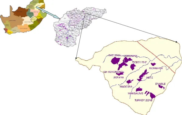
Figure 1. Location of the B72A quaternary catchment (showing village names) in the Olifants River

Basin, South Africa.

including the cyclic weather conditions, such as droughts. Family expenses and incomes, apart from the farming system are captured in the OLYMPE model, making it an appropriate tool to analyse total (farm plus non-farm incomes and food contribution) family food security. Further strength of this model is its participatory capabilities that allow contributions from farmers and other stakeholders in the database and scenario construction thereby boosting outputs confidence. In addition, the model offers possibility of linkages with other models, such as crop models. Based on the above strengths OLYMPE was adopted for use in this study.

Study area

The study area is located in B72A quaternary catchment (534 km2) in Ga-Sekororo area in the Olifants River Basin of South Africa (Figure 1). A quaternary catchment is the lowest water management area in South Africa. A large part of the catchment (80%) falls under the former Lebowa homelands. Homelands were areas set aside by the former apartheid regime for occupation by Africans. These areas were uneconomical and relied entirely on grants from the South African government (South Africa, 1998). The total population is estimated at 56,000 inhabitants (Statistics South Africa, 2001). The catchment is characterised by high population density, high poverty and unemployment levels.

The catchment climate is largely controlled by the

movement of air-masses associated with the Inter-Tropical Convergence Zone. Hence, the area experiences seasonal rainfall that largely occurs during the summer months, from October to April. The mean annual rainfall is 603 mm; with potential evapotranspiration rates above 1500 mm (actual evapotranspiration is around 840 mm) and the average maximum temperature of 270C (DWAF, 2004). The average farm sizes range from 0.5 to 2.5 ha and the soils (sandy loam and loamy sand) are poor (Rasiuba, 2007). Large commercial farms that provide some employment to the local community are located in the northern part of the catchment. In addition, recent government policies on Black Economic Empowerment (BEE) encourage and support smallholder farmers to ensure food security in the country. An example of such programs is the Rehabilitation of Small Irrigation Schemes (RESIS) program implemented by the Limpopo Department of Agriculture at provincial level to rehabilitate the small-scale irrigation schemes (DA, 2005).

The main crops grown in the study area under rainfed are maize, sugar beans, groundnuts, while spinach, cabbages green beans, beetroot, and tomatoes are grown under irrigation (Ntsheme, 2005). Maize that constitutes the staple crop for rural households is by far the most important crop in the area as it is grown by more than 80% of the farmers (Mapedza et al., 2008). Major agricultural risks in the area are related to fluctuation in weather conditions (low and erratic rainfall), resulting in high variability of crop yields (Magombeyi and Taigbenu,

(5)

2008), lack of formal credit facilities, unfavourable market arrangements (Fabre, 2006), lack of resources for cultivation and purchasing of mineral fertilisers (Kgonyane and Dimes, 2007). Detailed land and water management practices are described in Ntsheme (2005) and Mapedza et al. (2008). To realise farm level goals of sufficient family food, income and sustainable farming, continuous adaptation to aforementioned risks by farming systems is required.

MATERIALS AND METHODS

The main method employed to evaluate farming systems production performances is the OLYMPE model. The determination of the profitability of different farming systems comprised four steps, namely: 1) identifying and characterising farming systems in the study area, 2) defining the typical farming systems in the socio-economic model, 3) using a bio-physical model to determine yields for the farming systems, and 4) applying a socio-economic model to determine the financial effects under different climate and market price scenarios at farm-scale.

Farming systems construction

The study used data generated from two socio-economic surveys on farmers’ food security and irrigation sustainability carried out in 2005 by Nyalungu and Malajti in B72A quaternary catchment (Mapedza et al., 2008). The surveys adopted a stratified sampling technique in eight villages (Enable, Metz, Makgaung-Hafanie, Madeira, Ga-Sekororo, Sofaya, Tickyline and Worcester) in the study area, with a final total sample size of 159 farmers. On-farm experimentations (2005 to 2008) aimed at unearthing technical and social constraints; augmented information used for farming systems classification and provided inputs for the socio-economic model. The farm typologies were identified using multivariate analysis techniques (principal component analysis, correspondence analysis and cluster analysis) applied to the data to identify the most differentiating combinations of variables and their statistical relationships. Principal component analyses, based on correlations among variables and inertia of data, and cluster analyses, based on eight factorial coordinates were applied sequentially to establish preliminary farm typologies (Mapedza et al., 2008). Analysis of variance and F-test of the different farming systems established heterogeneity between the farm groups. Furthermore, group discussions with farmers, key non-governmental organisations (NGOs) personnel working with farmers, extension officers, and field observations complemented the surveys information and were used to validate the preliminary farm typologies.

The indicators used to differentiate the farming systems were farmland size, family size, cropping intensities, land to labour ratio, number of livestock units, total family balance, off-farm employment (Bezabih and Harmen, 1992), and input intensities of fertiliser and seed. Additional information on the cost of agricultural inputs/outputs was obtained from local shops in the study area.

Maize crop yield modelling

The relationships between rainfall and crop yields for each farm typology (crop production functions) required for farm simulations were deduced from observed data on maize crop yield, evapotranspiration and rainfall over three experimental years (2005 to 2008). The observed data were extrapolated using the Predicting Arable Resource Capture in Hostile Environments During the

Harvesting of Incident Rainfall in the Semi-arid Tropics (PATCHED-THIRST) crop model (Mzirai et al., 2001), calibrated for the study area (Magombeyi and Taigbenu, 2008).

OLYMPE software and farming system performance assessment

General description of OLYMPE model

OLYMPE software is a decision-support tool developed in France to improve the understanding of farming systems and socio-economic context of farmers (Attonaty et al., 1999). It can be applied to both individual and group farms. Penot et al. (2004) have applied the OLYMPE model as a farm database and management tool for commercial and subsistence farms in Indonesia. OLYMPE comprises farm and family accounts and computes all physical (inputs and outputs) and socio-economic (budgets, margins, incomes, cost-benefits, etc) variables over 10-year simulation periods up to 100 years. This provides data for a 10-year period adequate for policy analysis, as it is likely to cover good and bad years for both weather and market prices.

The family subsistence food requirements in terms of self-consumption of agricultural produce are incorporated in the model under family accounts. The simulations permit prospective analysis of the impact of volatility of prices and/or climatic events on crop and livestock production on a representative farm. All standard information that qualifies the structure and components of production factors of the representative farm are required. Such information includes cropping systems, labour, off-farm activities (crafts work and hawking) and cost of inputs/outputs. A detailed description of OLYMPE model features are presented in Attonaty et al. (1999).

Performance assessment indicators for farming systems

Performance evaluations of different farming systems based on annual gross margin (gross income at farm gate prices less variable costs) were carried out. The gross margin (output from OLYMPE) excludes farm’s fixed costs. Hence, it does not measure farm profit. The total net income is shown in Equation 1:

Net farm income + non-farm income = Total family income (1) Where net farm income variable is fixed costs subtracted from total farm income. Fixed costs remain constant irrespective of the level of output produced, such as depreciation of equipment and rent, while variable costs directly vary with the level of output, for example costs of fertiliser, seed and insecticide. Total family income less total family expenses, including, cost of family maize grain consumption, captured in OLYMPE family expenses account, gives the total family balance.

We defined farm resilience as the ability of a farming system to maintain a stable positive gross margin under adverse market prices and climate conditions, such as droughts and floods. Vulnerability that has find applications in hazard preparedness and poverty reduction (Magombeyi and Taigbenu, 2008), refers to the degree to which different farming systems (socio-economic classes) are differentially at risk and their ability to cope or recover from farming hazards to sufficiently meet their family food requirements. The key indicators of vulnerability to livelihood strategies at farm level are farm gross margin and total family balance.

Labour and return on investment ratio calculations from OLYMPE outputs: The ratio of total farm output to the number of

(6)

282 Afr. J. Agric. Res. 0 200 400 600 800 1000 1200 0 1 2 3 4 5 6 7 2008 2009 2010 2011 2012 2013 2014 2015 2016 2017 2018 In -s ea so n r a in fa ll ( m m ) Y ie ld ( t/ h a ) Year

Current fa rming pra ctices Chololo pits technology Ra infall

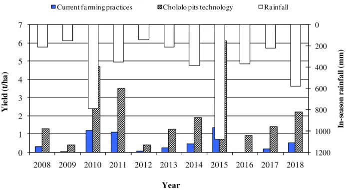
Figure 2. Maize yield variation under current and chololo pits or planting basins crop management practice. The average

(n = 10 years) yield is 0.5 and 2 t/ha for current and chololo pit practices, respectively. Rainfall was generated from Parched-Thirst model weather generator.

available family labour was based on an average throughout the whole year. The gain from a farm investment, subtract the cost of the investment, and divide by the total cost of the investment estimated the return on farm investment (Return on farm investment = (Gains – Cost)/Cost).

Recommended minimum household food expenditure

Family threshold income was calculated based on the recommended minimum daily dietary requirement of 2 261 kilocalories per person in South Africa (Bonti-Ankomah, 2001), and extrapolated to the family unit by the number and composition of family members (Dogliotti et al., 2005). Thus, the minimum per capita expenditure to meet this recommended dietary intake in South Africa was US$ 32 per month (2006). Hence, food expenditure for the farm family was adjusted to 2008 prices by an average (2005 to 2008) yearly food consumer price index of 10% in South African rural areas (Nkgasha et al., 2008). The annual minimum food expenditure for a farm family of five persons (Magombeyi and Taigbenu, 2008) in the study area was therefore, estimated at US$ 2 542 (2008), assuming that household expenditure grew by the yearly inflation rate.

Scenarios tested

Two types of scenarios were tested. The first set of scenarios compare the maize production and subsequent impact on economic farming systems performance under two different maize crop water management practices: current and improved crop water management practices (Figure 2) in the form of planting basins or

chololo pits. Both practices were tested under average and severe

drought/flood climatic conditions. The second set of simulations

analyse the impact of inputs (fertiliser and seed) and outputs (maize grain and livestock) price variation on farm performances, separately and combined. Under different scenarios analysed, other crops were kept at base-year (2008) production levels and prices. Simulations were performed over a 10-year period that covers different price variations and climate years, but these years are not necessarily the next 10 real years. Detailed scenario descriptions and simplifying assumptions are presented next and summarised in Table 1.

Maize yield variation under different production practices

Maize yields under current and improved planting basins crop management practices (Figure 2) were evaluated using PATCHED-THIRST crop model. The average (n = 10 years) yield is 0.5 t/ha and 2 t/ha for current and chololo pit practices, respectively. Rainfall (Figure 2) was generated from PATCHED-THIRST model weather generator . Current crop management practices involve ploughing, levelling and sowing maize seeds, while planting basins involve the digging of pits (0.22 m diameter, 0.3 m depth, spaced at 0.6 m within rows and 0.9 m between rows) and planting two to three maize seeds per pit (Mati, 2005). Planting basin practice captures and stores more rainfall than current crop management practice resulting in more water availability to crop roots and possibly higher yields. The maize crop yield variations due to climatic conditions only, were (7 to 249%) and (76 to 576%) of the long-term average maize yield of 0.5 t/ha in the area for current and improved planting basin production practices, respectively. This result indicates that planting basins improved the yields by more than fivefold in good rainfall years, while in poor rainfall seasons maize yield stabilised to about 76% (Figure 2) of long-term average yield, which is still better than the current practice. Hence, the risk of current crop management practice is higher compared to that of improved

(7)

Table 1. Summary of scenarios tested.

Variable Scenarios

1 2a 2b 2c 3a 3b 3c 4a 4b 5 6 Yields

Current management practices and average long-term yield X X X X X X X

Current management practices and climate variability X

Improved management practices and climate variability X X

Current and improved practices and extreme drought/flood conditions X

Maize grain price

2008 price X X X X X X X

Long term current trend X X

Low price X

High price X

Fertiliser and maize seed price

2008 price X X X X X X X X

Long term current trend X X

High price X

Cattle price variation X

0 50 100 150 200 250 300 350 400 1995 1998 2001 2004 2007 2010 2013 2016 2019 W h it e m a iz e p r ic e ( U S $ /t o n n e ) Year

Maize high price Maize low price Maize past & current price trend (NAMC, 2008) OECD-FAO (2008) outlook

0 0.5 1 1.5 2 2.5 3 1997 2000 2003 2006 2009 2012 2015 2018 P r ic e ( U S $ /k g ) Year

Fertiliser past & current price trend Fertiliser price-high price Maize seed past & current price trend (NAMC, 2008) Maize seed-high price

(a) (a)

Figure 3. a) Annual maize price variation scenarios under current trend, high price, low price OECD-FAO (2008) outlook. b) Maize seed and

fertiliser price scenarios for current trend and high prices.

practice of planting basins in the area.

Maize and fertiliser price variations

The yearly variations in market prices of maize grain, fertiliser (top dressing and basal; N = 3: P = 2: K = 1) and maize seeds were estimated for the simulation period (2008 to 2017) based on historic trends observed from 1990 to 2008 (NAMC, 2008; OECD-FAO, 2008; SAFEX, 2008). The choice to analyse fertiliser input was based on its largest (39.3%) contribution to total regional variable farm input costs (NAMC, 2008). Short-term (less than a year) price variability is excluded in this study. Four maize price scenarios were considered: current trend, high price, low price and OECD-FAO outlook (OECD-FAO, 2008). The high and low price series scenarios were derived from Monte Carlo simulations (van der Sluijs et al., 2004) using Microsoft Excel (Wittwer, 2004) based on historical prices. The highest historical price (US$ 190/tonne) was taken as the lower bound for maize high-price scenario, while the

upper bound was taken as twice the highest historical value (with the assumption that the price doubles). Under the low-price scenario, the prices for upper and lower bounds were taken as the lowest historical price (US$ 91/tonne) and twice the lowest historical price, respectively. Maize grain price-variation is defined in relation to the current maize grain price of US$ 228/tonne (2008) paid to farmers. Maize grain price ranges are 40 to 98% for the low price scenario, 84 to 121% for the current price trend, and 88 to 157% for high price variation (Figure 3a). The OECD-FAO outlook is not discussed further as the price variation lies between the low and high price scenarios. Maize price hikes are attributed to raising fuel prices, decreased production and competition from bio-fuel extraction.

Annual fertiliser and maize seed price scenarios under current and high price trends are presented in Figure 3b. The lower price bound was the 2008 price, while the upper bound was three and half times the 2008 price for high fertiliser and maize seed prices. Fertiliser price ranges are 100 to 267% and 88 to 157% of 2008 price of US$ 0.46/kg for current and high price trends, respectively.

(8)

The maize seed price ranges are 54 to 76% and 96 to 192% of the 2008 price of US$ 0.83/kg for current and high price trends, respectively. Different fertiliser producers tend to release new improved fertiliser types and various package sizes on the market for trials by farmers. Consequently, it is difficult to monitor the fertiliser prices due to continuous injection of new products into the market. Therefore, the fertiliser and maize seed price fluctuations depicted in Figure 3b only provides a general trend (NAMC, 2008).

In a more holistic approach, a combined scenario of input and output price variations was tested, where the farm outlook is assessed assuming planting basins crop management practice, with maize grain, fertiliser and maize seed prices following the current price trend.

The production behaviour of each farm typology was explained by the socio-economic farm characteristics. Results of gross margin and total family balance variations under different scenarios are reported in comparison to 2008 (base year) figures. According to 2008 exchange rate, 1US$ was equivalent to ZAR 9 (SAFEX, 2008). A summary of the scenarios is presented in Table 1.

Assumptions on scenarios

Under the different maize production scenarios, it was assumed that changes in maize yields are only due to changes in productivity of land as a result of new practices in water, land and crop management. There is an increase of maize production without yield quality changes under planting basins practice. Farm labour and crop area place limits on farm production, and were assumed to remain the same over the simulation period. There is no significant deterioration in soil quality, such as through erosion during the period of simulation.

Under maize-price variation scenario, other factors (costs of inputs, labour, productivity) were kept at base-year level (2008). Fertiliser-price variation simulations were executed without changes in applied fertiliser quantity or quality by the farmer, while other input costs were kept at the base-year level. For all the simulations, the crop types grown from each farming system or typology were assumed to remain constant. The number of family members on farm was assumed to remain constant over the simulation period. Finally, the physical conditions at farm scale are assumed to be spatially homogeneous.

RESULTS Farming systems

Five farming systems that encompass diverse cropping and livestock systems were identified in B72A quaternary catchment in the Olifants River Basin in South Africa. Their main characteristics, for instance, resource availability, input costs and minimum farm incomes are presented in Table 2. These farming systems depend on a combination of factors, such as environmental conditions (land quality and rainfall), and capital endowments, affected by socio-economic conditions of farmers. Hence, the different farming systems experience different constraints to technological innovations adoption. Off-farm incomes substantially complement agricultural incomes and influence the intensity of farming activities. Larger proportions (> 60%) of the farms were female-headed. These farms had more difficulties in feeding their families than the male-headed farms.

The most significant variables that distinguished the farm typologies appeared to be the number of hired workers, asset endowment (measured by an asset index, see Table 2 notes), number of livestock units, the sources of income, level of both crop and total family income, fertiliser use per hectare and crop diversity. Land area and proportion of income from irrigated crop, as well as seed costs per hectare were insignificantly different across farm typologies. (The farming systems presented in this paper are likely to evolve in the future (Landais, 1998; Perret, 1999).

Type A: Subsistence farmers with external jobs

The farmers acquire most of their income (> 70%) from non-agricultural employment and none from government grants. Agriculture supplement family food requirements and fertiliser usage is below average (80 kg/ha). These farmers grow both maize and vegetables crops and their livestock units (1.2) are below average (2.61) (Table 2).

Type B: Resource-constrained rainfed and irrigation farmers

The farmers are younger than the average age of farmers (54 years), with low levels of assets. Their land size is below average and manpower/ha is highest compared to all farm types. These farmers realise far below average total family income. Agricultural activities that contribute about 88% of family income support their main family needs, with half of this income coming from irrigation. They possess below average (1.12) livestock units, mainly goats (Table 2).

Type C: Social grant supported rainfed farmers

The farmers are supported by government through social grants (not necessarily used for their subsistence farming activities) and pensions that contribute 52% towards stabilizing the total family income. Both their total (family plus hired) manpower/ha of 3.3 capita/ha and fertiliser/ha use of 33 kg/ha are below the average values of 4.5 capita/ha and 80 kg/ha, respectively. Their cropping system is undiversified as they practice low levels of irrigation. However, they own above average (2.6) livestock units (Table 2).

Type D: Intensive, diversified irrigation farmers

These farmers derive most (67%) of their family income from diversified crops and livestock farming and use part of that money to buy large quantities of inputs, such as fertilisers (190 kg/ha) and seeds. High inputs and irrigation income, with slightly below average (1.3 ha)

(9)

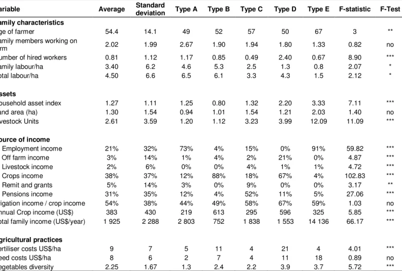
Table 2. Farming systems in the B72A quaternary catchment, Olifants River Basin. Data was derived from field surveys from 2005 to 2006.

Variable Average Standard

deviation Type A Type B Type C Type D Type E F-statistic F-Test Family characteristics

Age of farmer 54.4 14.1 49 52 57 50 67 3 **

Family members working on

farm 2.02 1.99 2.67 1.90 1.94 1.80 1.33 0.82 no

Number of hired workers 0.81 1.12 1.17 0.85 0.49 2.40 0.67 8.90 ***

Family labour/ha 3.40 6.2 4.6 5.3 2.5 1.3 0.8 2.07 *

Total labour/ha 4.50 6.6 6.5 6.1 3.3 4.3 1.5 2.12 *

Assets

Household asset index 1.27 1.11 1.25 0.80 1.32 2.20 3.33 7.11 ***

Land area (ha) 1.30 1.54 0.94 1.01 1.54 1.21 2.03 1.40 no

Livestock Units 2.61 3.59 1.20 1.12 3.23 3.99 12.09 11.09 ***

Source of income

% Employment income 21% 32% 73% 4% 15% 0% 91% 59.82 ***

% Off farm income 3% 14% 1% 4% 2% 21% 0% 4.87 ***

% Livestock income 2% 6% 0% 0% 4% 1% 1% 4.72 ***

% Crops income 38% 37% 12% 88% 18% 67% 4% 102.83 ***

% Remit and grants 5% 14% 3% 0% 9% 0% 0% 3.17 **

% Pensions income 31% 35% 12% 4% 52% 11% 5% 27.06 ***

Irrigation income / crop income 54% 38% 44% 49% 58% 67% 59% 1.03 no

Annual Crop income (US$) 383 430 219 613 295 596 325 5.85 ***

Total family income (US$/year) 1 925 2 288 2 803 752 1 838 1 553 14 136 66.17 ***

Agricultural practices

Fertiliser costs US$/ha 9 7 5 11 4 21 4 4.01 ***

Seed costs US$/ha 8 6 2 7 4 11 18 0.89 no

Vegetables diversity 2.25 1.67 1.3 2.4 2.2 3.9 3.7 5.72 ***

Sample size (N) = 159 farmers; 2. 1 US$ = 9 ZAR (2008).; 3. *** F- test significant at 99 %, **; F test significant at 95 %, no: not significant at 90%; 4. Type A: Subsistence farmers with external jobs; Type B: Resource-constrained rainfed farmers; Type C: Social grants supported rainfed farmers; Type D: Intensive, diversified irrigation farmers and Type E: Rich, salaried entrepreneurs - very extensive farmers. 5. Off-farm income refers to income from self jobs such as hawking, craft work, brewing beer and excludes salaried employment; 6. The household asset index was calculated from standardised scores (0 to 5) based on the type, size, construction material of the house (s) at the homestead, farming implements and in-house items such as cooking stoves, furniture, etc.; 7. Vegetable diversity was calculated based on the number of vegetable crops grown by the farmer.

land size confirm their intensive farming activities. These farmers are younger than an average farmer age (54 years) (Table 2). Hence, they are likely to be receptive to innovations.

Type E: Rich, salaried entrepreneurs-very extensive farmers

The farmers represent a small proportion (2%) of farmers in the area that obtain most of their income (> 90%) from non-agricultural employment. Their crop income only contributes 4% of total family income, while an average for all farm types is 38%. They are the richest farmers, with highest asset index of 3.3 and livestock units of 12.1,

accumulated over the years. In addition, they own largest (2.0 ha) pieces of land, but the land is not fully utilized because household heads are engaged in other non-agricultural activities. An average farmer age is greater than 67 years. Hence, farmers are old, labor constrained and reluctant to engage in crop production. Maize production is not important to these farmers as they mostly practice vegetable farming for self-consumption (Table 2).

Farming system performance under average historical maize yields (Scenario 1)

(10)

286 Afr. J. Agric. Res. -150 -50 50 150 250 350 450 550 650 750 850 950

Type A Type B Type C Type D Type E

Farm Type

U

S

$

Gross margin Net income

-2000 0 2000 4000 6000 8000 10000

Type A Type B Type C Type D Type E

Farm Type

U

S

$

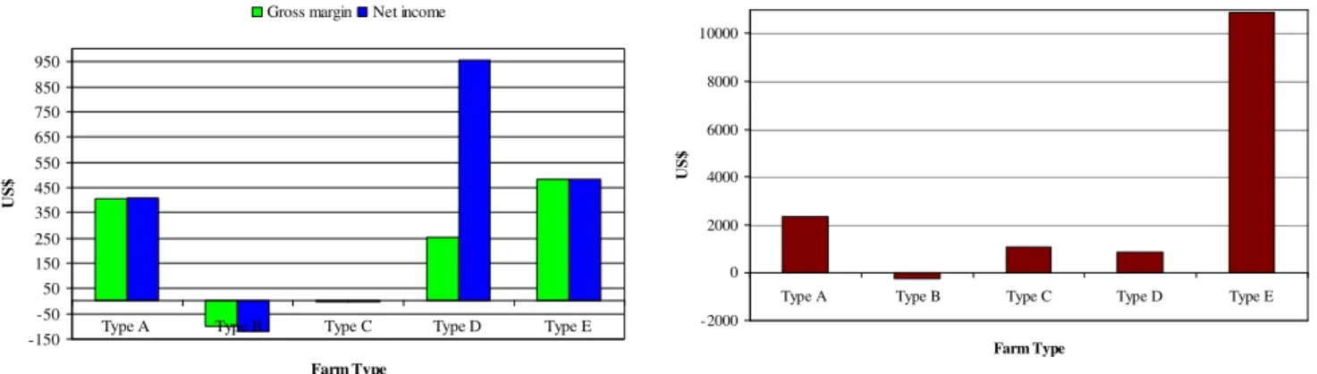
Figure 4. a) Average (5 years) annual farm gross margin and net income. b) Average annual (5 years) total family balance.

Table 3. Base year labour and indicator ratios for the farm types calculated from OLYMPE model results and Table 2.

Variable Farming systems

Type A Type B Type C Type D Type E

Labour requirement/crop season (hours) 259 284 416 363 53

Farm size (ha) 0.94 1.01 1.54 1.21 2.03

Total workers available (family + hired) 7 6 3 4 2

Hired workers 1 1 0 3 1

Used labour/season (h/ha) 276 281 270 300 26

Shortage of labour No No No Yes No

Total farm expenses (US$) 429 472 519 680 244

Total farm outputs (US$) 833 371 518 934 727

Farm gross margin (US$) 405 -100 -1 253 482

Farm gross margin (US$/ha. year) 430 -100 0 209 238

Return on labour (US$/capita. year) 119 62 173 233 363

Return on investment ratio 0.9 -0.2 -0.002 0.4 2

years) yields varies from –US$ 902 to US$ 481 (Figure 4a), while the total family balance variation was from – US$ 218 to US$ 10 857 (Figure 4b). Farm Types B and C performed poorly as indicated by their negative gross margin, implying variable production costs exceeded gross farm income. Therefore, these farms are economically unsustainable in low yield years as 2008 (Figure 2). However, farm Type A, had a positive total family balance (US$ 1 098) because most of the family income (73%) is realised from employment outside farming (Table 2); implying that the agricultural component of this production system is unsustainable.

Farm Type B experienced a negative (–US$ 100) total family balance; implying food shortage by this amount. Hence, farm Type B needs to source income outside farming to secure family food security. This negative total family balance could be a stimulus to farm Type B to change to better farming practices to mitigate against crop failure or take up employment elsewhere. Farm Type E had the highest gross margin mainly from sales of high livestock units (Table 2). Farm Types E and Type A, with the highest and second highest total family balances

(Figure 4b), respectively, are most resilient to crop failure than other farm types as they do not depend much on crop production. The results seem to indicate that gross margin from livestock production is more stable than from crop production, especially in dry years.

Manpower required (man days) for farm activities including the available labour and return on investment ratios (Table 3) were calculated from OLYMPE model results and farm systems characteristics (Table 2). Type E, the livestock keepers showed the highest return on labour (US$ 363/capita.year) followed by Type D (US$ 233/capita. year) and Type C (US$ 173/capita. year). Farm Type A had the highest gross margin/ha because of the small cultivated area (Tables 2 and 3). The return on investment ratios ranged from –0.2 for farm Type B to 2 for farm Type E. Farm Type E had the highest return on investment ratio, followed by farm Type A (0.9) and farm Type D (0.4), with diversified crops and few livestock units. High return on investment ratios are desirable as they indicate that expenses are lower relative to the revenue they produced. An investment (farming system) without a positive return on investment ratio should not

(11)

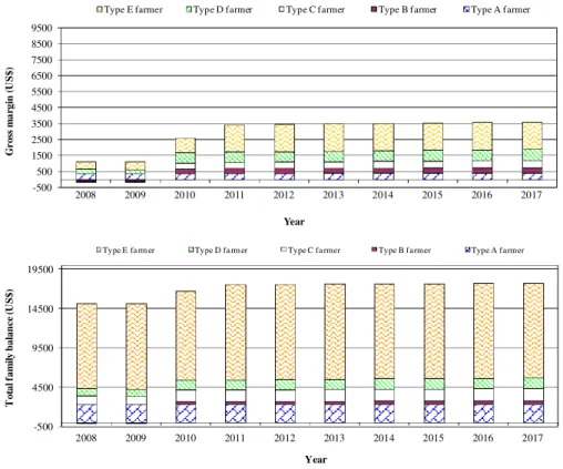
-500 500 1500 2500 3500 4500 5500 6500 7500 8500 9500 2008 2009 2010 2011 2012 2013 2014 2015 2016 2017 G r o ss m a r g in ( U S $ ) Year

Type A farmer Type B farmer Type C farmer Type D farmer Type E farmer

-500 4500 9500 14500 19500 2008 2009 2010 2011 2012 2013 2014 2015 2016 2017 T o ta l fa m il y b a la n c e ( U S $ ) Year

Type E fa rmer Type D farmer Type C fa rmer Type B fa rmer Type A fa rmer

Figure 5. a) Projected annual gross margin under current maize crop management and rainfall. b) Projected total family balance

under current maize crop management and rainfall.

be undertaken. Return on investment ratios of less than 1 is very risk, while a return on investment of 2 is resilient. However, when these ratios are too high, it is difficult to tell whether it is because of a combination of low revenues and expenses.

Farm Types B and C had the lowest labour return and return on investment ratios, implying farm diversification and intensification could be desirable strategies to resuscitate these two farming systems. However, the object of choosing a crop management technique can be decided based on family labour availability. If the available labour is exceeded, it becomes important to know when and by how much additional labour cost is required.

Farming systems comparison under different maize production practices (Scenarios 2)

Farming systems performance under current crop management practices (Scenario 2a)

Gross margin and total family income variations under current crop management practice are presented in Figure 5a and b, respectively. Farm Type B performed worst, with gross margin range of –US$ 180 to US$ 434, while Type E performed best, with gross margin range of US$ 478 to US$ 896 (Figure 5a). Farm Type D performed second best with gross margin range of US$ 148 to US$ 828 (71 to 394%) (Figure 5a) and family balance range of 75 to 139%) (Figure 5b) compared to 2008 figures. The negative gross margin is indicative of unprofitable farming practice and possibly a strain in family food security. Hence, farm Type B needs to look for income elsewhere to meet the shortfall required to satisfy the family needs. Farm Type E gross margin is insignificantly affected by the variability in maize yields, as it is based on livestock production. Livestock production was less affected by the erratic rainfall distribution and dry spells responsible for poor crop yields, except in extreme drought conditions.

However, it was noted that farm Type D was no longer

second best under family balance (Figure 5b), but farm Type A, because of the larger employment contribution (73%) to family income (Table 2). This result indicates the possibility for farm-based households to earning higher total gross margin and annual family income than households with full-time employed members, in good rainfall years. The drastic drop in gross margin in 2009 (Figure 5a) was due to a severe drought (Figure 2) or a major disaster, such as flood that cause enormous damage to both crop and livestock productions, consequently reducing food security. All farm types recovered in the subsequent year, but sometimes it may take two to three years recovering from such devastating disasters because of resource limitations to rehabilitate damaged infrastructure.

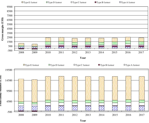
Farming systems performance under planting basins practice (Scenario 2b)

Gross margin and total family balance for maize productions under planting basins scenario are shown in Figure 6a and b, respectively. The annual yield variations under planting basins were presented in Figure 2. These planting basins are also known as chololo pits in western Kenya. Farm variations based on 2008 figures were: Type A gross margin (76 to 192%), total family balance (98 to 119%); Type B gross margin (–177 to 412%), total family balance (–218 to 699%); Type C gross margin (– 18 to 815%), total family balance (86 to 186%); and Type D gross margin (55 to 368%), total family balance (82 to 205%). Gross margin and total family balance variations for Type E were (98 to 209%) and (100 to 104%), respectively. The total family balance variations for farm Types A and E were insignificantly changed compared to the current management practice results (Figure 5a and b). Farm Type B performed worst under this scenario, as shown by both negative gross margin (Figure 6a) and total family balance (Figure 6b) in the first two years of simulation. However, planting basins practice out-performed the current crop management practices for farm Types A to D, even during the severe drought year

(12)

288 Afr. J. Agric. Res. -500 500 1500 2500 3500 4500 5500 6500 7500 8500 9500 2008 2009 2010 2011 2012 2013 2014 2015 2016 2017 G ro ss m a rg in ( U S $ ) Year

Type E farmer Type D farmer Type C farmer Type B farmer Type A farmer

-500 4500 9500 14500 19500 2008 2009 2010 2011 2012 2013 2014 2015 2016 2017 T o ta l f a m il y b a la n ce ( U S $ ) Year

Type E farmer Type D farmer Type C farmer Type B fa rm er Type A fa rmer

Figure 6. a) Simulated farm gross margin under chololo pits or planting basins practice and rainfall variation. b) Projected farm total family

balance under planting basins practice and rainfall variation.

-2500 -500 1500 3500 5500 7500 9500 2008 2009 2010 2011 2012 2013 2014 2015 2016 2017 G ro ss m a rg in ( U S $ ) Year

-500 4500 9500 14500 19500 2008 2009 2010 2011 2012 2013 2014 2015 2016 2017 T o ta l f a m ily b a la n ce ( U S $ ) Year

Type E fa rmer Type D fa rmer Type C fa rmer Type B fa rmer Type A fa rmer

Figure 7. a) Projected annual farm gross margin under low maize production. b) Projected

farm total family balance under low maize production.

of 2009 and consistently reduced both gross margin and total family balance variability during the 10-year simulation period, with 2010 and 2011 as best years (Figure 6a and b). Hence, planting basins can significantly improve food security provided a threshold rainfall amount is received.

Farming systems performance under severe

drought/flood (Scenario 2c)

Farming systems performance under a severe drought or flood, assumed to be experienced in 2009 (scenario 2c),

when no maize grain was harvested is shown in Figure 7a and b. This scenario was of interest as the Limpopo Province, where Olifants River Basin is located, is under constant threat from El Nino conditions, such as the cyclone experienced in 2000. These cyclone floods reduced crop yields to below 20% of an average long-term yield (0.5 t/ha) and in some areas caused complete crop failure.

A sharp drop in gross margin (Figure 7a) and a decrease in total family balance (Figure 7b) were observed in the cyclone year (2009) for all the farm types, with farm Type B most affected (gross margin of –US$ 359 and total family balance of –US$ 291). Under farm

(13)

-500 500 1500 2500 3500 4500 5500 6500 7500 8500 9500 2008 2009 2010 2011 2012 2013 2014 2015 2016 2017 G ro ss m a rg in ( U S $ ) Year

Type E fa rm er Type D fa rm er Type C fa rmer Type B farmer Type A farmer

Figure 8. a) Projected annual farm gross margin under current trend maize price

variation. b) Projected farm total family balance under current trend maize price variation.

Types A (US$ 405) and Type E (US$ 483), gross margin declined by 55 and 22%, respectively, compared to 2008 figures. Farm Type C had the largest negative gross margin value (–US$ 428), implying that the farmer had the largest loss on the farm enterprise. However, farm Types C and D had positive total family balance of US$ 670 and US$ 612, respectively, due to cushioning by additional farm family income from pensions, remittances and grants (Table 2). Total family balances declined by 9, 732, 38, 31, and 1% for farm Types A, B, C, D and E, respectively. This percentage decline represents the loss in total family food security resulting from maize grain production.

The results indicate the importance of supplementing total farm balance from other sources outside farming, such as employment. This appears to be a viable livelihood strategy in drought and flood-prone Olifants River Basin. Farm Types A and E realise more than 70% of their family income from employment, while social welfare grants from government serve as safety nets for farm Types C and D (Table 2). The vulnerability of farm types to severe drought starting with the most vulnerable is B, C, D, A and E. Farm Type B is most vulnerable because it derives about 88% (Table 2) of its total family income from crop production and without safety nets. For farm Types E and D, livestock consistently stabilised farm gross margin, though both farm types revealed susceptibility to extreme events, such as floods and extended droughts that could destroy livestock or reduce

livestock price due to poor health. Therefore, under these extreme events, all farmers have difficulty in feeding their families solely from farm production. Social support, as either food or cash from both government and donors, enhance access to food supply by the resource-constrained farmers.

In comparison to other shocks in a farming system, severe drought/flood results in most decrease in gross margin and total family income, partly due to loss of production for farm family consumption. This production loss triggers increased expenditure in buying food from the market and consequently, price hikes of maize grain at local and regional markets. Similarly, timing of Asian monsoon rains that affect crop yields impact price variability of agricultural commodities (OECD, 1999). OECD-FAO (2008) and OECD (1999) argued that in the past years, production shortfalls in cereals by exporting countries set a stage for global rapid price hikes.

Farming systems performance under maize grain price scenarios

Farming systems performance under current maize grain price trend (Scenario 3a)

Gross margin and total family balance variation under current maize grain price trend are shown in Figure 8a and b. Gross margin ranges were 96 to 105% and –113

(14)

Type E fa rm er Type D fa rm er Type C farm er Type B farmer Type A fa rm er

-500 4500 9500 14500 19500 2008 2009 2010 2011 2012 2013 2014 2015 2016 2017 T ot a l f a m ily b a la n ce (U S $ ) Year

Type E fa rmer Type D fa rmer Type C farmer Type B fa rmer Type A fa rmer

Figure 9. a) Projected annual gross margin under low maize price variation. b) Projected total family

balance under low maize price variation.

to 318% for farm Types A and B, respectively. Farm Type D showed highest range in total family balance of 98 to 149%, due to high maize yields. Total family balance ranges for farm Types A and E of 99 to 101% and 100 to 111%, respectively, were insignificantly impacted by maize price variation compared to farm Types B and C that rely mostly on maize crop production (Table 2). The total family balance (Figure 8b) showed a similar trend to farm gross margin variations (Figure 8a).

Farming systems performance under low maize grain price trend (Scenario 3b)

Gross margin and total family balance variations under low maize price scenario (Figure 3a) are presented in Figure 9a and b. The low price scenario mostly affected farm Types B and C as they derive most of their family income from agriculture and pensions, respectively (Table 2). Farm Type D performed best on gross margin because of its crop diversification (vegetables, groundnuts and sugar beans) and intensive farm practices (Tables 2 and 3) that compensated for low maize prices. The results indicate that crop diversification

can reduce vulnerability to family food insecurity.

Farming systems performance under high maize grain price trend (Scenario 3c)

Gross margin and total household balance variations under high maize price scenario (above US$ 228) (Figure 3a) are presented in Figure 10a and b. Least variation (10 to 29%) in gross margin under farm Type A was noted (Figure 10a) compared to the 2008 figures. Total family balance for both farm Types B and C ranged from –72 to 154%. These two farm types were most affected as they experienced negative gross margin and total family balance (Figure 10a and b). Hence, farm Types B and C are most susceptible to maize grain price inflation shocks, while farm Types D and E are the most resilient. High livestock units (12.09) (Table 2) that were liquidated to provide cash, made farm Type E the most resilient to maize price shocks, while for farm Type D, it was crop diversification. On comparison of the three maize grain price variation scenarios, we noted that farmers are mostly susceptible to low maize grain price inflation shocks.

(15)

Type E farmer Type D fa rmer Type C fa rmer Type B farmer Type A farmer

Type E fa rmer Type D fa rm er Type C fa rmer Type B fa rm er Type A farmer

Figure 10. a) Projected annual gross margin under high maize price variation. b) Projected

annual total household balance under high maize price variations.

According to literature surveyed, it is still not clear how long-term regional food security is affected by increase in food prices (that differ across regions) intended to stimulate crop production, such as maize. Most price shocks are induced by production shortfalls resulting from weather disturbances (OECD, 1999), increases in petroleum prices that push up agriculture production costs through increased costs of inputs, such as fertilisers and machinery. Social protection, argued by the African Union, if provided from on-budget resources in developing countries in the form of social transfers would enhance purchasing power and effective demand, and create a long-term production stimulus for resource-constrained smallholder farmers (OECD, 1999). However, social protection can result in increased price variability to both producers and consumers in countries open to trade.

Farming systems performance under different fertiliser price trends

Farming systems performance under current

fertiliser price trend (Scenario 4a)

The fertiliser price variations under current and high trends were presented (Figure 3b). Farm Type D, with the highest fertiliser use (190 kg/ha) (Table 2) showed variations of (100 to 260%) and (100 to 145%) in gross

margin (Figure 11a) and total family balance (Figure 11b), respectively. Farm Types B and C were most affected as they apply fertiliser in irrigated plots that produce half of their family income, while Farm Type A was unaffected because of its low fertiliser usage (Table 2).

Farming systems performance under high fertiliser price trend (Scenario 4b)

Comparing the scenarios of fertiliser under current (Figure 11a and b) and high (Figure 12a and b) price trends, we noted that in both scenarios the fertiliser price variation (Figure 3b) did not impact gross margin and total family balance for farm Type A, due to its low fertiliser usage. The percentage change in total family balances for all the farms were the same for the two scenarios compared to 2008 figures, due to small quantities of fertiliser usage, except farm Types D and B that use 190 and 95 kg/ha, respectively (Table 2). For these two farm types the gross margin varied by 160 and 205% for farm Types D and B, respectively. Consequently, the total family balances for farm Types D and B changed by 45 and 37%, respectively. The result indicates insignificant effects of fertiliser price changes on total family balance, where little fertiliser is used. This result is supported by a reduction in fertiliser applications by smallholder farmers as fertiliser prices rise.

(16)

292 Afr. J. Agric. Res. -500 500 1500 2500 3500 4500 5500 6500 7500 8500 9500 2008 2009 2010 2011 2012 2013 2014 2015 2016 2017 G ro ss m a rg in ( U S $ ) Year

Type E fa rm er Type D fa rmer Type C fa rmer Type B fa rmer Type A fa rmer

Type E fa rmer Type D fa rmer Type C farmer Type B farmer Type A fa rm er

Figure 11. a) Projected annual gross margin under current fertiliser price trend. b) Projected

annual total family balance under current fertiliser price trend.

Type E farmer Type D fa rmer Type C fa rmer Type B fa rmer Type A fa rmer

Type E fa rmer Type D farmer Type C fa rmer Type B fa rmer Type A fa rm er

Figure 12. a) Projected annual gross margin under high fertiliser price trend. b)

(17)

-500 500 1500 2500 3500 4500 5500 6500 7500 8500 9500 2008 2009 2010 2011 2012 2013 2014 2015 2016 2017 G r o ss m a r g in ( U S $ ) Year

-500 4500 9500 14500 19500 2008 2009 2010 2011 2012 2013 2014 2015 2016 2017 T o ta l f a m il y b a la n c e (U S $ ) Year

Figure 13. a) Projected annual gross margin under cattle price variation scenario. b)

Projected annual farm balance under cattle price variation scenario.

Developments in the bio-fuel markets had a noticeable influence on fertiliser prices as they influence the international demand for fertilisers and availability of fertiliser input materials. An agricultural policy that ensures the poorest rural farmers have access fertiliser at reasonable prices will enhance agricultural production.

Farming systems performance under cattle price variation (Scenario 5)

The price per beast was varied from US$ 333 to US$ 778 (US$ 556 as the base price). Farm type gross margins (Figure 13a) varied according to the following ranges: A (80 to 151%), D (–114 to 889%) and E (80 to 488%), compared to 2008 values. Farm Types B and C had highest changes in gross margin, due to their few livestock units, compared to other farm types. The total family balance varied according to the following ranges: Type A (14 to 39%), B (–600 to 36%), C (–9 to 119%), D (32 to 251%) and E (4 to 22%), compared to 2008 values. Gross margin and total family balance were lowest in the drought/flood year of 2009. The gross margin is highest under the cattle price variation scenario compared to all scenarios investigated.

Farming systems performance under combined planting basins, future rainfall and current price trend for both fertiliser and maize grain (Scenario 6)

The combined effect of planting basins practice, future rainfall and current price trend for both fertiliser and maize grain is presented in Figure 14a and b. The gross margin (Figure 14a) varied according to the following ranges for farm Types A (74 to 177%), D (52 to 344%) and E (98 to 188%) compared to 2008 figures. Farm Type B and C had the highest gross margin variation (more 700%). The total family balance (Figure 14b) varied according to the following ranges for farm Types A (95 to 116%), B (–240 to 719%), C (83 to 176%), D (82 to 184%) and E (100 to 104%) compared to 2008 figures. The results show high variability in gross margin compared to total family balance. Farm Types A and E show variation in total family balance of 19 and 4%, respectively, indicating that these farm typologies are not directly affected by agricultural production changes at farm level. Farm Types B, C and D could hardly secure enough food for their families from 2008 to 2017 (Figure 14b). Farm Type E maintained a stable gross margin as livestock prices were not affected by both fertiliser and maize grain price variations. Total family balance for farm

(18)

294 Afr. J. Agric. Res. -500 0 500 1000 1500 2000 2500 3000 2008 2009 2010 2011 2012 2013 2014 2015 2016 2017 G ro ss m a rg in ( U S $ ) Year

Type A farmer Type B farmer Type C farmer Type D farmer Type E farmer Family food needs

-2000 0 2000 4000 6000 8000 10000 12000 2008 2009 2010 2011 2012 2013 2014 2015 2016 2017 T o ta l f a m il y b a la n ce ( U S $ ) Year

Type A farmer Type B farmer Type C fa rmer Type D fa rmer Type E fa rmer Minimum family food needs

Figure 14. a) Projected annual gross margin under combined scenario of planting basins

practice, future rainfall variation, current fertiliser and maize grain price trends. b) Projected annual total family balance under combined scenario of planting basins practice, future rainfall variation, current fertiliser and maize grain price trends.

Types B, C and D remained lowest throughout the 10-year simulation period compared to other farm types, due to their crop based farming systems. Farm types E and A (6 out of 10 years) are likely to meet the minimum family food requirements, while farm Types B, C and D show shortfalls (Figure 14b). However, even for the richest farmers (A and E), the family food requirements cannot be met by agriculture alone (Figure 14a), suggesting the need for farmers to engage in other off-farm activities to broaden and supplement their farming livelihood strategies.

DISCUSSION

The socio-economic-agronomic model presented in this article is considered to be a useful instrument for assessing the resilience or vulnerability of different farming systems based on farm gross margin and total family balance. For a realistic farm level modelling, we distinguished different categories of family farms (typologies), based on finance, resource endowments and farming practices. Furthermore, the strengths and weaknesses of the different farming systems were considered to provide an insight into the highly variable

farm investments and management strategies that are often observed in smallholder farmers.

The cultivated fields of 0.9 to 2 ha from the farm typologies are comparable to four smallholder farm typologies (based on resource endowments and objective of farming) of farm sizes 0.5, 0.9, 1.2 and 2.8 ha, found in western Kenya (Africa NUANCES, 2007). Sole crop production farming systems present more risks to the farmers than livestock system or mixed (crop and livestock) farming systems. Hence, the introduction of livestock (cattle, goats, and sheep) into the farming systems stabilises income and builds family capital (Table 2) that provides a buffer to both climatic and market price shocks. Nonetheless, excessive livestock ownership in fragile landscapes should be avoided as it may exacerbate land degradation by overgrazing.

It must be noted that relationships and trends are more important than absolute figures, as the model presented only covered specific groups of farmers in the study area. The modelled scenarios reflect indicative maize price variations that are assumed to follow certain distributions and historical trends. Hence, the forecasts by the model should be considered indicative, as input variables might differ from actual future values. Data and variables used in constructing the farming systems were obtained from