HAL Id: hal-02054206
https://hal.sorbonne-universite.fr/hal-02054206
Preprint submitted on 1 Mar 2019
HAL is a multi-disciplinary open access
archive for the deposit and dissemination of
sci-entific research documents, whether they are
pub-lished or not. The documents may come from
teaching and research institutions in France or
abroad, or from public or private research centers.
L’archive ouverte pluridisciplinaire HAL, est
destinée au dépôt et à la diffusion de documents
scientifiques de niveau recherche, publiés ou non,
émanant des établissements d’enseignement et de
recherche français ou étrangers, des laboratoires
publics ou privés.
Modelling the Effect of Mass-Draining on Prominence
Eruptions
Jack M. Jenkins, Matthew Hopwood, Pascal Démoulin, Gherardo Valori,
Guillaume Aulanier, David M. Long, Lidia van Driel-Gesztelyi
To cite this version:
Jack M. Jenkins, Matthew Hopwood, Pascal Démoulin, Gherardo Valori, Guillaume Aulanier, et al..
Modelling the Effect of Mass-Draining on Prominence Eruptions. 2019. �hal-02054206�
MODELLING THE EFFECT OF MASS-DRAINING ON PROMINENCE ERUPTIONS
JACKM. JENKINS,1MATTHEWHOPWOOD,2, 3PASCALD ´EMOULIN,4GHERARDOVALORI,1GUILLAUMEAULANIER,4
DAVIDM. LONG,1 ANDLIDIA VANDRIEL-GESZTELYI1, 4, 5
1Mullard Space Science Laboratory, University College London, Dorking, RH5 6NT, UK;jack.jenkins.16@ucl.ac.uk 2School of Mathematics, University of Birmingham, Birmingham B15 2TT, UK
3School of Mathematical Sciences, The University of Adelaide, Adelaide, SA 5005, Australia 4LESIA-Observatoire de Paris, CNRS, UPMC Univ Paris 06, Univ. Paris-Diderot, Meudon Cedex, France
5Konkoly Observatory of the Hungarian Academy of Sciences, Budapest, Hungary
(Received January 1, 2018; Revised January 7, 2018; Accepted January 23, 2019)
Submitted to ApJ ABSTRACT
Quiescent solar prominences are observed to exist within the solar atmosphere for up to several solar rota-tions. Their eruption is commonly preceded by a slow increase in height that can last from hours to days. This increase in the prominence height is believed to be due to their host magnetic flux rope transitioning through a series of neighbouring quasi-equilibria before the main loss-of-equilibrium that drives the eruption. Recent work suggests that the removal of prominence mass from a stable, quiescent flux rope is one possible cause for this change in height. However, these conclusions are drawn from observations and are subject to inter-pretation. Here we present a simple model to quantify the effect of “mass-draining” during the pre-eruptive height-evolution of a solar flux rope. The flux rope is modeled as a line current suspended within a background potential magnetic field. We first show that the inclusion of mass, up to1012kg, can modify the height at which
the line current experiences loss-of-equilibrium by up to 14%. Next, we show that the rapid removal of mass prior to the loss-of-equilibrium can allow the height of the flux rope to increase sharply and without upper bound as it approaches its loss-of-equilibrium point. This indicates that the critical height for the loss-of-equilibrium can occur at a range of heights depending explicitly on the amount and evolution of mass within the flux rope. Finally, we demonstrate that for the same amount of drained mass, the effect on the height of the flux rope is up to two order of magnitude larger for quiescent than for active region prominences.
Keywords: Sun: filaments, prominences — Sun: fundamental parameters — Sun: atmosphere — Sun: magnetic fields
1. INTRODUCTION
Coronal mass ejections (CMEs) are complex bundles of magnetic field and material that erupt from the solar atmo-sphere out into the helioatmo-sphere. A key feature often mea-sured within their interplanetary counterpart is a rotation of the magnetic field vector as spacecraft cross the magnetic structure, a property believed to be indicative of a magnetic flux rope (e.g., Burlaga 1988; Palmerio et al. 2017; James et al. 2017). In addition, the existence of a flux rope in the so-lar atmosphere has often been related to the formation of fil-ament systems; elongated structures observed in absorption on the solar disk (Priest et al. 1989;Aulanier et al. 1998). Filaments are interpreted as strands of dense material sus-pended in the low-coronal atmosphere. Such structures are historically identified as prominences when observed above the limb, and we shall henceforth use the term prominence to
describe these structures, unless otherwise indicated. The ob-servational signature of the on-disk counterpart, a filament, provides no immediate evidence for the suspended nature of the material above the solar surface (van Ballegooijen & Martens 1989;Martin 1998;Gibson et al. 2006;R´egnier et al. 2011). Prominences have been observed for up to several solar rotations, occasionally within a coronal cavity when a prominence quasi-parallel to the equator is projected above the limb. A pre-eruptive flux rope has been suggested to ex-ist in equilibrium for equally extended periods of time (Rust 2003;Gibson et al. 2004).
Despite being typically stable features within the solar at-mosphere, the final stages of a prominence’s life are highly dynamic; the suspended plasma either drains back to the chromosphere, or is ejected into the heliosphere as the core of a CME, or some combination of both (Dere et al. 1997;
Schmahl & Hildner 1977;R´egnier et al. 2011). In the erup-tive case, the sudden destabilisation of these structures is also indicative of the destabilisation of the host flux rope. The ex-act causes for the loss-of-stability of a flux rope are under-stood to depend on the conditions under which the flux rope formed and the recent evolution of the surrounding magnetic field (Moore et al. 2001;Lynch et al. 2004;T¨or¨ok & Kliem 2005;Fan & Gibson 2007). Unfortunately, flux ropes are not directly observable in the solar atmosphere as they are mag-netic in nature and instrumentation sensitive enough to accu-rately measure the coronal magnetic field does not yet exist (although preliminary attempts are being made, e.g., Ba¸k-Ste¸´slicka et al. 2013;Fan et al. 2018). Therefore, in order to effectively study the stability criteria of flux ropes, a com-bination of observations (e.g.,Zuccarello et al. 2014,2016), extrapolations (e.g.,James et al. 2018), and simulations (e.g.,
Fan 2017) are typically used (see alsoCheng et al. 2017, and references therein). The simulations are often employed to study the cause of the loss-of-stability of a flux rope in the lead-up to its eruption, with the observations and extrapola-tions separately offering information about the pre-eruptive configuration.
Before the advent of advanced simulations, early work by van Tend & Kuperus (1978) presented a 2D analytical model in which the flux rope was approximated as a straight line current suspended at equilibrium in a background po-tential magnetic field. Although a simplified setup was em-ployed, the authors qualitatively demonstrated that increas-ing the magnitude of the line current causes its height above the solar surface to increase. This relationship between the current and height of the line current can be represented with an equilibrium curve. In addition, they concluded that there is a point at which an increase in the strength of the line current would no longer result in a solution on the equilib-rium curve. At this time, the line current was said to have experienced ‘loss-of-equilibrium’. Extensions to this model were employed to quantitatively study the balance of forces involved with prominences, and the evolution of this bal-ance prior to an eruption (e.g.,Low 1981;D´emoulin & Priest 1988;Martens & Kuin 1989;D´emoulin et al. 1991;Forbes & Isenberg 1991). However, authors such asMartens & Kuin
(1989) andD´emoulin et al.(1991) noted that the influence of the gravity term was negligible assuming “typical” values for prominence mass, and was unlikely to be able to perturb the equilibrium dominated by the magnetic pressure and tension forces.
More recently, work has been carried out to take this sim-ple line-current approach further and formulate more com-plex, time-dependent magnetohydrodynamic (MHD) simula-tions (for a more complete review on the state of these MHD simulations, seeCheng et al. 2017, and references therein). These models contain more physically realistic initial and
boundary conditions that allow the construction, evolution, and analysis of a fully 3D flux rope. Importantly, the mod-ern simulations have aligned with the conclusions of authors such asMartens & Kuin(1989) andD´emoulin et al.(1991) that the evolution of the magnetic field in and around a flux rope is assumed to be solely responsible for its evolution in time (D´emoulin 1998). Specifically, this low-beta approx-imation assumes that the pressure and mass of prominence plasma suspended by a flux rope is negligible in compari-son with the magnetic pressure and tension forces of the flux rope and its surroundings (Titov & D´emoulin 1999;Filippov 2018). Indeed, this assumption is featured frequently in three decades of modern research.
However, novel observations and hydrostatic modeling are beginning to suggest that mass may be able to influence the local and global properties of magnetic flux ropes (Low et al. 2003;Petrie et al. 2007;Seaton et al. 2011;Gun´ar et al. 2013;
Bi et al. 2014;Reva et al. 2017;Jenkins et al. 2018). In partic-ular, the Shafranov shift as explored inBlokland & Keppens
(2011) details how varying the gravity term in their 2D mag-netohydrostatic (MHS) model can cause the axis of their flux rope to decrease the height. Then, the mass-unloading theory (e.g.,Low 1999;Forbes 2000;Klimchuk 2001) has been sug-gested as one possible cause for the eruption of prominences. In this theory, a particularly heavy prominence suddenly un-loads all of its mass, reducing the gravitational force acting on the host flux rope and causing it to spring off into space as an eruption.
The study of the role of mass evolution within prominence eruptions has typically been isolated to a handful of obser-vational case studies. Seaton et al.(2011) presented stereo-scopic observations of a prominence erupting from an ac-tive region in which plasma was observed to unload from the prominence prior to its expansion in height. The authors con-cluded that in the absence of additional, contrary evidence, these observations were an example of a ‘mass-unloading’ eruption driver.
Recently,Jenkins et al.(2018) also presented stereoscopic observations of a quiescent prominence’s partial eruption in which ‘mass-draining’ was suggested to have been respon-sible for the accelerated expansion of the erupting magnetic flux rope. In this case the drained mass does not ultimately drive an eruption, it simply modifies the balance of forces acting on the prominence to a non-negligible degree (see also
Reva et al. 2017). Their conclusion that the mass-draining accelerated the eruption was reached through a quantitative estimation based on the Lorentz force equation, specifically the ratio between the modification of the gravitational force due to the reduction in mass and the force of the background magnetic tension restricting the height-evolution of the flux rope. However, this order of magnitude estimate to the
im-portance of the mass-draining does not properly account for the equilibrium conditions of the host flux rope.
Therefore, in this manuscript, we present an extension to the model developed byvan Tend & Kuperus(1978) that en-ables the study of the role of mass in the evolution of a line current in quasi-equilibrium. Specifically, we first explore how the inclusion of mass can modify the stability criteria for a line current that represents a flux rope suspending a promi-nence. We then explore how the removal of mass (or “drain-ing”) from a pre-eruptive line current, can modify the global height of the line current within the solar atmosphere. The general model is described in Sections2and3, and applied in Section4to a bipolar background potential magnetic field. In Section5, we further constrain the model with measure-ments made from the observations presented by bothSeaton et al.(2011) andJenkins et al.(2018). Finally, a discussion and summary are presented in Section6.
2. MODEL CONCEPT
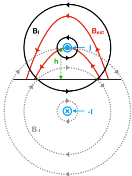
Following the formulation outlined in D´emoulin & Aulanier (2010), hereafter DA10, a flux rope is modeled in cartesian coordinates as a magnetic field generated by an infinitely long, straight line current I at a given height h above the photosphere. The justification for the choice of a straight line current over a curved line current lies in the assumed property of quiescent prominences being oriented largely horizontal to the surface. The majority of curvature may be assumed to be localised at the footpoints of the host magnetic flux rope that are located far from the center of the prominence. An “image” line current -I is introduced under the photosphere that runs anti-parallel to the “real” line cur-rent. Followingvan Tend & Kuperus(1978), the additional image magnetic field beneath the surface results in no mod-ification to the vertical, z, component of the photospheric magnetic field. This “image” current acts to increase the height of the “real” line current. The straight line current is then added to a background potential magnetic fieldBext
that acts to force the line current towards the photosphere. A cartoon representation of these different field contributions is shown in Figure1. The total field has an inverse configu-ration because of the presence of a flux rope (e.g., similar to the configuration of Figure 1a withinPetrie et al. 2007). The line current is then in equilibrium if the sum of forces is zero,
Â
f =0$ fu= fd)IB I= IBext (1)where fuis the sum of the upward magnetic forces, the
so-called hoop force, fdis the sum of the downward magnetic
forces, I ( I) is the real (image) current, Bext is the
hor-izontal background magnetic field component orthogonal to the current at heighth, and B Iis the strength of the
mag-netic field as a consequence of the image line current. The
I -I BI B-I Bext h
Figure 1. Cartoon diagram of the model set-up. The inverse mag-netic configuration is formed by the superposition of three fields: the external potential fieldBext(solid-red), and the field generated
by the line current (located at z=h) and its image (located at z=-h), drawn with solid-black and dashed-grey lines respectively. The line current at z=h is maintained by the balance of two Lorentz forces, an upward (hoop) force due to the magnetic field generated by the image line current, and a downward force from a stabilizing exter-nal potential fieldBext. Model concept is identical to that presented
byvan Tend & Kuperus(1978).
image magnetic fieldB Iis derived from Amp`ere’s law,
I
B I·dl=µ0I,
)B I= 2pRµ0I, (2)
where the strength of the magnetic fieldB Iis measured at
a point in space that is at a distance/heightR = 2h away from the line current, and µ0is the permeability of free space
equal to4p ⇥ 10 7in MKS units.
In order to simulate the existence of a prominence within a flux rope, thevan Tend & Kuperus(1978) model is extended to include mass that is set to exist at the same point as the line current, i.e., at heighth. The inclusion of mass into the system results in an additional downward force that acts to further anchor the line current. In equilibrium, Eq. (1) be-comes,
IB I=IBext+mg, (3)
wherem is the mass of the suspended plasma per unit length andg is the acceleration due to gravity. g is taken indepen-dent ofh (since h⌧r , where r is the solar radius) except where explicitly stated. All quantities in Eq. (3) are defined positive.
3. GENERAL EQUATIONS 3.1. Equilibrium Current
Here we will establish the general form of equations that will be applied to a specific Bext in the following sections.
The force f on the line current, per unit length, is,
f = µ0I
2
4ph IBext mg, (4) where Bext is a function of h (as well as other parameters
depending on the selected model). We setBext > 0 so that
the external magnetic field creates a force oppositely directed to the hoop force, µ0I2/4ph, and an equilibrium exists in the
limitm=0.
The electric current needed for equilibrium is given by solving Eq. (4) forI with f =0,
Ieq,m= 2phBext µ0 ± s✓2phB ext µ0 ◆2 +4p µ0m g h , (5)
where we have added the lower indexm to indicate that the equilibrium current depends on the mass.
With finite mass, Eq. (5) provides two equilibria corre-sponding to the sign selection in front of the square root. With a negative sign selected,Ieq,m<0, which implies that
both magnetic forces are upward and opposite to the gravity force in Eq. (4). This case has a vanishing current in the limit of a vanishing mass and it does not correspond to a force free equilibrium with a flux rope. Therefore, we consider only the second case with a positive sign in front of the square root of Eq. (5), Ieq,m= 2phBext µ0 + s✓2phB ext µ0 ◆2 +4p µ0 m g h , (6)
Supposing thatBext(0) is finite, then for small enoughh
values such thath⌧ (µ0m g/pB2ext),
Ieq,m⇡ 2phBext
µ0 +
s 4p
µ0 m g h . (7)
Then,Ieq,m(h) has a square root dependence withh when h is
small enough andm>0. This behavior changes to a linear dependence whenm=0.
With m = 0, Ieq,0(0) = 0, and since Bext typically
decreases faster than 1/h for large h values, Ieq,0(h) =
(2p/µ0)hBextwill tend towards zero at large heights. This
implies that Ieq,0(h)has a maximum (at least one) between
small and large heights. However, ifm>0, Ieq,m(h)is
dom-inated by the gravity term at largeh values once Bexthas
suf-ficiently decreased, then Ieq,m(h) ⇡ p(4p/µ0)m g h is a
growing function ofh for constant g. At even larger h values, asg is inversely proportional to(r +h)2, thenIeq,m(h)will
again tend towards zero, even for large mass values. Never-theless, for low enoughm and h values, Ieq,m(h) will still
have a minimum ath=0 and large heights, and a maximum
(at least one) somewhere in between. It is the response of the line current to mass within this region that we focus on during this study.
3.2. Dependence of the Equilibrium current on Mass We investigate below the effect ofm on Ieq,mkeeping all
other quantities fixed,
∂Ieq,m
∂m = g h
r
(hBext)2+µ0
p m g h 0 . (8)
Increasing the massm requires that the magnitude of the cur-rent is increased so as to reach a given height (i.e., to increase the hoop force).
Next, supposingm g h ⌧ (p/µ0)(hBext)2, a first order
Taylor expansion of Eq. (6) provides,
Ieq,m⇡Ieq,0+m g/Bext. (9)
Then, the equilibrium current is comparatively increased by adding a term proportional to the mass and to1/Bext. Since
Bext(h)is typically a decreasing function ofh, this implies
thatIeq,mis increasingly separated fromIeq,0with height.
3.3. Mass-draining
Finally, we will analyse the effect of draining prominence mass on the host flux rope’s equilibrium height and, possibly, its eruption. We suppose that the draining is fast enough that there is a negligible evolution, through e.g., diffusion (e.g.,
van Driel-Gesztelyi et al. 2003), of the vertical component of the photospheric field distribution. This is modelled with the image current and implies that the associated potential field, Bext, is unchanged. We suppose also that this
short-term evolution is done without reconnection. This implies that the magnetic flux,F, passing below the flux rope bottom (located atz=h a, where a is the radius of the flux rope / line current) and the photosphere (atz=0) is conserved.
van Tend & Kuperus(1978) suggested that a line current would experience loss-of-equilibrium if the current magni-tude exceeded the maximum of the Ieq,0(h)curve, as with
a classical electric circuit. DA10 (see alsoD´emoulin et al. 1991;Lin et al. 2002) expanded on this by imposing a short-term MHD evolution with flux conservation to study the loss-of-equilibrium of a flux rope. The hybrid MHD / line current approach uses pseudo-time long-term evolution of model pa-rameters, e.g., photospheric flux density f or average coronal twistT, to overcome the limitations of the classical approach. The evolution of one of the model parameters in this way al-lows the construction of a family of constantF curves which describe the short-term evolutions. The intersection of these
curves withIeq,0details how a flux rope evolves as a function
of the evolving parameter.
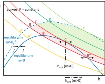
Two equilibrium curves, Ieq,m(h)andIeq,0(h)are shown
in Figure2together with five curves of fixed magnetic fluxF, differing from each other as a result of an evolution in, e.g., Bext. Assuming that we start with a nearly potential coronal
configuration, the prominence and its flux rope are supposed to first evolve quasi-statically along the stable equilibrium curve ofIeq,m(h), with a height growing slowly with time as
a result of the evolution ofBext. At some point during this
evolution, we have supposed that the draining of the full mass occurs fast enough to keep bothBextandF unchanged, then
the evolution is along the correspondingF=constant curve towards larger heights. The general form of theF=constant curve (Eq. (9) of DA10), hereafter defined asIevol(h)is,
Ievol(h) = L2 s 0 @F+ ZZ S Bextdy dz 1 A , (10)
whereLs = µ0pDy(ln(2h/a) +li/2),li, are the external
in-ductance, and normalised internal inin-ductance, respectively, anda is the radius of the current channel. For this set-up in which the current is focused at the edges of the current chan-nel,li =0.
The effect of draining the mass depends on the location where it occurs. If it occurs at point A of Figure 2, or a nearby one, then a stable equilibriumIeq,0exists at the
inter-section with theIevolflux curve (at point A0). Comparing the
height of stable equilibrium with and without mass linked by the sameIevol curve, the equilibrium with mass is always at
a lower height (e.g., hA < hA0) which is due to the
down-ward gravity force compressing the Bext configuration. As
the draining point is shifted to larger heights, e.g., at point B, the new equilibrium onIeq,0curve is further away, at a larger
height, from the initial one on Ieq,mcurve. This is the case
until the point C where theIevol flux curve only touches the
Ieq,0equilibrium curve tangentially. Equation (20) of DA10
demonstrates that the equilibrium is linear neutral at this tan-gent point C0, but it is unstable with the non-linear
pertur-bation term taken into account (graphically the Ievol curve
is extending to the right in the region where the force f is pointing towards largeh values, so away from the equilib-rium curve).
After the mass-draining occurs at a point such as A, the to-tal magnetic force will be directed upward, accelerating the flux rope towards the equilibrium curveIeq,0. However, this
equilibrium will be reached with a finite kinetic energy, al-lowing the line current to continue evolving along the Ievol
curve. The line current will then continue on the other side of the equilibrium point with a change in sign of the total magnetic force. Finally, at some point, the motion will stop and reverse direction leading to an oscillation of the flux rope.
hcrit(m>0) h I equilibrium m>0 A B C D f f B’’ C’ B’ E equilibrium m=0 curves F = constant A’ A’’ hcrit(m=0)
Figure 2. Schema showing the possible evolutions with mass-draining. The equilibrium curve withm = 0, Ieq,0(h), is shown
with a continuous dark blue line. The equilibrium curve with mass, Ieq,m(h), is above with a dashed line. The constraint of magnetic
flux conservation, Eq. (12), is shown with the other colored curves representing different starting points along Ieq,0(h) for draining
mass. If the draining mass starts between points C and E, no equi-librium can be reached without mass (region shaded in light green), while if draining is realized before point C (e.g., at point A), an-other stable equilibrium could be reached. In the region shaded in pink, the finite kinetic energy accumulated may allow the line cur-rent to reach the unstable equilibrium without mass (such as point B00). The small black arrows indicate the direction of the total force
when the line current is slightly shifted away from the equilibrium curve. The critical height(s)hcritof them=0 (m>0) line current
is indicated with the vertical (horizontal) black-dash-dotted lines.
This scenario also envisages damped oscillations towards the Ieq,0curve as the extra energy is progressively radiated away
by fast MHD waves. Such results have been reported in both 2D and 3D numerical simulations of prominence oscillations (e.g.,Schutgens & T´oth 1999;Zhou et al. 2018, respectively). Furthermore, theIevolcurve can also cross the other branch
of theIeq,0 curve past the point C0, such as at points A00and
B00in Figure 2. Since this part is unstable (see f arrows in
Figure2), there is the possibility of an eruption if the system has sufficient energy to reach this unstable part. This region is indicated qualitatively with a pink area in Figure2. Its ex-tension towards the side with smallh values is limited by the ability of the magnetic force to decrease the kinetic energy before the unstable region, at largerh values, is reached. We will not study this aspect any further since it is expected to be an effect localised to the family ofIevol curves near to point
C0 and this would need a detailed analysis (it depends both
onm and Bext(h)). We only point out that an eruption may
to the limiting curveIevolthat passes the first unstable point,
C0, of theIeq,0curve.
3.4. Modification of the Equilibrium Height In this subsection, we give a quantitative estimate of the ideas described with Figure 2. Specifically, we analyse the mass-draining from the equilibrium located at(hm, Im)with
massm, to the equilibrium located at(h0, I0)without mass.
The total flux passing between the bottom of the flux rope and the surface is,
F(h) = µ0I 2p ln ✓ 2h a ◆ Z h a 0 Bext(z)dz . (11)
Conserving flux passing below the flux rope per unit length Dy during the mass-draining requires that F(hm) = F(h0),
hence, Z hm a 0 Bext(z)dz µ0 2p Imln(2hm/a) = Z h0 a 0 Bext(z)dz µ0 2p I0ln(2h0/a), (12) where we suppose that the flux rope radius,a, is small com-pared to its height, and that a remains unchanged by the mass-draining to simplify the expressions as evolution ina has a low effect on the results (similar to the case m = 0 in DA10 where a did not evolve). Equation (12) explicitly states that the two equilibrium are on the sameIevol(h)curve
(Eq. (10))
We next suppose that the two equilibria (hm, Im) and
(h0, I0)are close enough, so that the mass has a small effect
on the force balance (m g h ⌧ (p/µ0)(hBext)2). We also
take the equilibrium without mass as a reference to express all terms of the Taylor development and define the variation quantities: Dh = h0 hm,DI = I0 Im. From Figure2,
Dh>0 and DI<0.
With a Taylor development to first order inDh and DI of Eq. (12), the conservation of flux imposes the relationship,
Dh h0 = µ0 2p ln(2h0/a) DI I0 . (13)
The equilibrium curve without mass satisfies,
0= µ0I
2 0
4ph0 I0Bext(h0), (14)
and the force balance with massm satisfies, D f = µ0I
2 m
4phm ImBext(hm) m g . (15)
With DI rewritten as a function of Dh with the flux con-served, Eq. (13), with I0 = (4p/µ0)h0Bext(h0), the first
order expansion around(h0, I0)of Eq. (15) is,
D f= m g+Dh4p µ0 B 2 ext (16) 1+ 2p µ0ln(2h0/a)+ ∂ln Bext(h) ∂ln h h=h0 ! .
Withm=0, Eq. (16) describes the test of stability of the equilibrium around the point(h0, I0). Next, we introduce the
notations,
n= ∂ln Bext(h)
∂ln h h=h0 , (17)
for the negative logarithmic derivative of the external field component, commonly referred to as the decay index ( Bate-man 1978;Filippov & Den 2001;T¨or¨ok & Kliem 2005; Zuc-carello et al. 2016), and,
ncrit=1+µ 2p
0ln(2h0/a), (18)
which is Eq. (33) of DA10 (withna = 0 since we have a
fixeda value). Then, Eq. (16) is rewritten as,
D f = m g+Dh4p
µ0 B 2
ext(ncrit n). (19)
With m = 0, the equilibrium at(h0, I0) is stable if D f is
oppositely directed to the displacement Dh from h0tohm.
This is achieved forn<ncrit, as expected.
Supposing that the extra energy is somehow dissipated, i.e.,D f =0, Eq. (19) also describes the mass-draining from the equilibrium at (hm, Im) to the equilibrium at (h0, I0).
This draining implies the shift in height, Dh= 4p m g
µ0 B
2
ext(ncrit n), (20)
to the new equilibrium(h0, I0) which exists only for n <
ncrit. This quantifies the graphical description of Figure2.
In particular, it shows thatDh is proportional to the loaded massm and inversely proportional to distance, in terms of decay index, to the loss-of-equilibrium point (n=ncrit).
Fi-nally, the strength of the external field has a strong effect on Dh since a factor 10 on Bext decreasesDh by a factor 100
(this factor 10 onBextis the order of magnitude for the
ra-tio between the field present in active and quiescent promi-nences for example). We conclude that the draining of a given massm could cause the height of the prominence to increase from a tiny to a very large amount (up to the loss-of-equilibrium and resulting eruption) depending on precisely where this draining occurs along the equilibrium path and on the strength of the external field.
4. RESULTS
4.1. Bipolar Background Field
We begin by expanding on the case investigated in DA10 to explore the effect of including mass on the evolution of the
Figure 3. Equilibrium curves demonstrating Eq. (24), the relationship between electric current magnitude and height of the line current suspended within a bipolar background potential magnetic field generated by a 4 G mean surface field. These equilibrium curves are calculated assuming a range of prominence mass between107 –1010 kg Mm 1. The dotted-black line corresponds to no mass within the system,
comparable to the solid-black line in Figure 2c ofD´emoulin & Aulanier(2010).
line current, suspended within a bipolar background mag-netic field, up to its loss-of-equilibrium. Here, the bipolar background magnetic field is supplied by two, infinitely long polarities at distance±D from the position of the line cur-rent (DA10),
Bext=2fD(p(h2+D2)) 1, (21)
where f is the magnetic flux per unit length in the invariant direction. Substituting Eqs. (21) and (2) into (4), we arrive at the condition for the system in equilibrium with f =0,
µ0I2
4ph
2fDI
p(h2+D2) mg=0 . (22)
The equilibrium curve for the massless line current is, Ieq,0(h)
Ipeak = ˜Ieq,0(˜h) =
2˜h
(˜h2+1), (23)
whereIeq,0(h)is normalised by its maximum value,Ipeak=
f
p, occurring at height ˜hpeak = hpeak/D = 1. Note that
Equation (23) corrects a typo of DA10. For the case where a line current does contain mass, ˜Ieq,m(˜h)takes the form
sim-ilar to Eq. (6), ˜Ieq,m(˜h) = 2p 2˜hD µ0f Bext+ r (Bext)2+ µ0mg p ˜hD ! . (24)
In Figure3we show a comparison between normalised equi-librium curves of line currents suspended within a “typical” quiet-Sun region of average surface field strength equal to 4 G and loaded with a range of masses. The properties of the masses used are presented in Table1, assuming a typi-cal quiescent prominence of dimensions: length=100 Mm, height=30 Mm, width=4 Mm (Labrosse et al. 2010;Xia et al. 2012).
NH(Total) Mass (Total) Mass (Per unit length)
(cm 3) (kg) (kg Mm 1)
5⇥107 109 107
5⇥108 1010 108
5⇥109 1011 109
5⇥1010 1012 1010
Table 1. The properties of the masses loaded onto the line currents presented in Figure3. It is assumed that all mass within a promi-nence is cool (low ionisation ratio), therefore NH is the number
density of neutral hydrogen assuming the range of masses within the second column (Labrosse et al. 2010).
4.2. Effect of Mass on Line Current Equilibrium Here, we impose the same flux evolution analysis, de-scribed in Section3.3, on the equilibrium curves presented in Figure3to study the effect of mass on the equilibrium of the host line current.
The reference state with fluxes ˜F0 and f0 is defined at
the maximum of the ˜Ieq,0(˜h)curve (DA10, and references
therein),
˜F0= 2pµ0˜Ipeakln 2˜hpeak˜a
!
2tan 1⇣˜hpeak ˜a
⌘ , (25) where ˜Ipeak is the maximum value of ˜Ieq,0(˜h), and ˜a is the
normalised radius of the line current (˜a= a/D=0.1
here-after). We readily find ˜Ievol(˜h)from Eq. (10),
˜Ievol(˜h) = ˜F+2tan
1 ˜h ˜a µ0 2pln ⇣2˜h ˜a ⌘ , (26) where ˜F= ˜F0/ ff.
Figure 4. The effect of mass on the stability of a line current suspended within a bipolar background potential field. Panel a; intersection of ˜Ieq,0(˜h)and ˜Ievol(˜h)with ff = 1 indicating two equilibrium positions, ˜h = 1, 1.33, as in Figure 2c ofD´emoulin & Aulanier(2010).
Panel b; orange, green, and blue curves correspond to the last point-of-intersect, with ff decreasing, between ˜Ieq,m(˜h)and ˜Ievol(˜h), with
ff =0.986, 0.973 and 0.869 for line currents loaded with mass equal to 0, 109, and1010kg Mm 1, respectively. The vertical magenta-dotted
lines indicate theh/D value for this last intersection, in each case, between the two ˜I(˜h)curves.h/D value is seen to increase as more mass is loaded.
The intersection of ˜Ievol(˜h) and ˜Ieq,0(˜h) for the case of
ff = 1 for the massless line current is shown in
Fig-ure4a. The orange curve in Figure4b then corresponds to ff = 0.986 (1.4% reduction in f0, the strength of the
pho-tospheric polarities) applied, also, to the case of a massless line current, indicating a single point of intersection between the two ˜I(˜h)curves, ath/D =1.15. Any further reduction in ffresults in no intersection between the two ˜I(˜h)curves.
DA10 demonstrate that such a line current experiences an ideal-MHD instability and an outward force drives the erup-tion of the line current.
In Figures3 and 4b it is shown that an increase in the amount of mass loaded onto the line current results in a shift in the maximum value ofI/Ipeakand its correspondingh/D
value. As with the orange curve, the green and blue curves are the last point of intersect between ˜Ieq,m(˜h)and ˜Ievol(˜h)
where a line current is loaded with109and1010kg Mm 1,
respectively. This implies that the flux of the photospheric polarity must decrease further than for the massless case in order for the mass-loaded line current to experience an ideal-MHD instability. For a line current loaded with 109
or1010kg Mm 1, ideal-MHD instability occurs after f has
decreased by 2.7% and 13.1%, respectively, at a height of h/D = 1.17, 1.32. Therefore, the simple model presented here appears to demonstrate that a mass-loaded line current can be significantly anchored as a result of the inclusion of mass (cf. Blokland & Keppens 2011), requiring additional current within, photospheric flux decay below, and height for the line current to experience loss-of-equilibrium.
Fan(2018) recently published the first example in which a prominence comprised of mass on the order of 1012 kg
erupted in a fully MHD simulation. Interestingly, the exis-tence of this prominence was shown to have a significantly stabilising effect on its host flux rope when compared to an
identical flux rope without prominence formation induced. Specifically, the prominence was shown to inhibit the initia-tion of the kink instability prior to a successful erupinitia-tion. The work presented here shows that a similar conclusion can also be reached with the torus instability using significantly sim-plified conditions.
4.3. Effect of Mass-Draining on the Pre-Eruptive Evolution of the Line Current
Blokland & Keppens(2011) showed that the inclusion of mass within their MHS model caused the center of their flux rope to be pulled downwards i.e., the Shafranov shift. Further to this, we have established that the inclusion of mass within the simple model presented byvan Tend & Kuperus(1978) and expanded by DA10, can result in a non-negligible modi-fication to the equilibrium curves and implies additional sta-bility. It is therefore reasonable to suggest that the removal of this mass from a pre-loss-of-equilibrium line current will also result in a modification to its evolution, as suggested in sev-eral observational case studies of prominences (e.g.,Seaton et al. 2011;Bi et al. 2014;Reva et al. 2017;Jenkins et al. 2018).
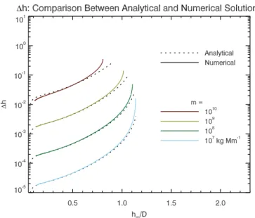
To test this hypothesis and simulate the draining of promi-nence mass from a flux rope, we first apply the general, first-order development described in Section3.3, specifically Eq. (20), to the specified bipolar background magnetic field of Eq. (21). The results are presented in Figure 5 as the dashed-black lines. Dh is larger when hm is closer to the
loss-of-equilibrium point (i.e.,n=ncrit). However, Eq. (20)
is derived with a Taylor expansion in Dh, so it cannot de-scribe largeDh values.
Therefore, we have used the “Chebfun” package (see,
Driscoll et al. 2014) implemented in MATLAB to solve nu-merically for the intersects between ˜Ieq,m(˜h), ˜Ieq,0(˜h), and
˜Ievol(˜h)for a range of values of ff. These solutions are
pre-sented in Figure 5, plotted over the analytical solution for comparison. Although the main trend is accessible via both the analytical and numerical solutions, the numerical solution emphasises the sensitivity of the equilibrium to mass evolu-tion when the line current is close to its loss-of-equilibrium.
5. IMPLICATIONS FOR OBSERVATIONS We now move to establish a basic comparison between the results of the above model and two specific observations of mass-draining. Our model shows that some of the quantities may be very sensitive to the value used in their computation, see e.g., Figure5for largehm/D. The model input
parame-ters (filament dimensions, height, mass, and external field as a function of time) require indirect, often complex methods to be estimated from observations, and are subject to differ-ent types of errors. Therefore, our intdiffer-ention is to establish an order of magnitude indication to the importance of mass-draining in these two cases, not an exact measure. Further-more, we find that varying the value ofa/D between 0.1 and 0.5 results in modifications to the stability of the line current of only a few %. Therefore, for this comparison we maintain the assumption of a the thin flux rope and fixa/D=0.1.
We first refer to a recent case study byJenkins et al.(2018) in which the authors used the column density estimation tech-nique ofWilliams et al.(2013) andCarlyle et al. (2014) to study the draining of mass from an erupting quiet-Sun promi-nence. According to the authors observations, shortly prior to the prominence’s eruption the total mass within the field-of-view reduced by at least 1⇥1010kg, equal to 15% of the
initial mass within the field-of-view. The additional proper-ties of the erupting prominence were estimated from observa-tions taken using the Atmospheric Imaging Assembly (AIA;
Lemen et al. 2012) on board the Solar Dynamics Observatory (SDO;Pesnell et al. 2012),
D=65 Mm Ly =260 Mm BPhot =4.6 G f= pDBPhot 2 dm=1 ⇥ 1010kg
where Ly is the length of the prominence. Specifically, D
is half the width, and Ly the length, of the red-dashed box
in Figure 3b ofJenkins et al.(2018). The value ofBPhot is
the average strength of the magnetic field within the bounds of the red-dashed box in Figure 3a ofJenkins et al.(2018). The results of the application of these values to the model are shown in Figure6.
In the application of the observations to this model we have set initial mass equal to 9⇥1010kg and final mass equal to
Figure 5. The change in the height of a line current due to a range of mass-draining, assuming a bipolar background potential magnetic field generated by an average surface field of strength 4 G. Analyt-ical solutions to Eq. (20) are plotted for each mass as dashed-black lines. Overplotted on these dashed lines are the solid-coloured lines representing the numerical solution. The analytical solution works well for smallh and m values, but clearly deviates from the numer-ical solution at larger values.
8 ⇥1010 kg. According to the model, such a mass-loaded
line current would need to reach a height of⇡75 Mm to lose stability,⇡30 Mm higher than the prominence top was ob-served; the quiet-Sun prominence was suggested to lose equi-librium, inferred by the large acceleration, after it had risen to a height of⇡45 Mm. In fact the comparison between model and observations cannot be precise because of the approxi-mate values derived from observations and the simplicity of the model. Moreover, all of the mass present in the model ex-ists at the height of the line current, a location representative of the axis of a flux rope. As it is commonly assumed that prominence material resides below this height, in the dips of the magnetic field of a flux rope (e.g.,Aulanier et al. 1998;
Gun´ar & Mackay 2015), we expect the model height cor-responding to loss-of-equilibrium to always be larger than any observed prominence height (see also,Zuccarello et al. 2016).
The increase in height observed byJenkins et al.(2018) af-ter the prominence underwent mass-draining was>60 Mm before leaving the field-of-view. The simple model described here predicts the maximum possible increase in height for the same amount of mass-draining to be up to 1.7 Mm, as-suming the final state is also in equilibrium. However, it is suggested by the authors that the flux rope associated with the prominence was at a point of marginal instability when the mass-draining initiated. Indeed, we have shown that the
simple model described here predicts the largest increases in height due to mass-draining to occur as the line current ap-proaches its loss-of-equilibrium. Hence, the large increase in the height of the observed prominence (60 Mm) shortly after the draining of mass could be interpreted as being caused by the flux rope losing equilibrium and erupting into the helio-sphere due to the torus instability. The prominence observed byJenkins et al.(2018) did successfully erupt and was later observed as a CME by multiple coronagraphs.
The mass estimates of the prominence material studied by
Jenkins et al. (2018) were derived from observations cap-tured using the Extreme Ultraviolet Imager (EUVI;Wuelser et al. 2004) on board the Solar Terrestrial Observatory Be-hind (STEREO;Kaiser et al. 2008) spacecraft. At the time of the observations, December 2011, EUVI was capturing high temporal resolution images in only the 195 ˚A passband; the other filters were at a much lower cadence. For this reason, the column density of the prominence was calculated using the so-called ‘monochromatic method’, resulting in a lower-limit estimate to the column density. Therefore, we take the derived value of total mass and mass-drained as lower-limits, and in turn all values ofDh to be lower-limit estimates to the increase in the height of the line current.
Next, we compare to an earlier case study, presented by
Seaton et al.(2011), in which it was concluded that mass-draining from a prominence rooted within an active region was responsible for the ⇡ 35 Mm height rise prior to the eruption of the prominence. The active region that the eruptive prominence was located in was in its decaying phase, with an average surface magnetic field strength of
&100 G according to magnetogram observations taken using the Michelson Doppler Imager (MDI;Scherrer et al. 1995) on board the Solar and Heliospheric Observatory (SOHO;
Domingo et al. 1995). Our model can be used to test this conclusion by assuming the same degree of mass-draining as was observed byJenkins et al.(2018), and modifyingBPhot
so as to test the sensitivity of the model to a range of surface fluxes.
In the solar context, higher values of BPhot are
associ-ated with smaller values ofD, in turn reducing the critical height of the flux rope. Indeed, this is a commonly observed and well studied relationship between prominence height and magnetic domain (e.g.,Rompolt 1990;McCauley et al. 2015;
Filippov 2016, and references therein). However, in order to meaningfully vary D with BPhot within this model,
ad-ditional assumptions would have to be made. Therefore, to facilitate a simple comparison between the two observational case-studies and the additional range of realistic surface flux values, we opt to compare conditions for a “normalised fila-ment”, fixingD as inJenkins et al.(2018) and simply varying BPhot.
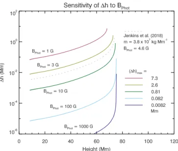
Figure 6. The modification to the height of the line current assum-ing a drainassum-ing equal to 1⇥1010 kg of prominence mass
(Jenk-ins et al. 2018) at a range of photospheric magnetic field strengths. Quiet-Sun surface field strengths result in a significantly larger change in height due to mass-draining than field strengths similar to those observed in active regions.
The results, shown in Figure6, suggest that increasing the surface magnetic flux results in a stronger background poten-tial magnetic field, and reduces the effect that mass-draining can have on the height changeDh. According to the model, draining 1⇥ 1010 kg from a line current embedded within
a bipolar background potential magnetic field that has a sur-face magnetic field strength of& 100 G would result in a very small maximum change to the height of the line current unless the configuration is very close to loss-of-equilibrium. It is therefore unlikely that the mass-draining was directly re-sponsible for the observed⇡35 Mm increase in the height of the prominence. Nevertheless, as appears to have been the case in the prominence studied byJenkins et al.(2018), the mass-draining may have been responsible for upsetting the equilibrium towards the non-equilibrium point.
A similar result to this has previously been reported by
Reeves & Forbes (2005), in which the authors concluded the effect of mass was likely to be negligible in a system re-stricted by a background field stronger than 6 G. Our result is complementary to this by providing a quantitative compar-ison for a range of surface fluxes and masses.
6. DISCUSSION AND SUMMARY
The general cases described in this manuscript detail how the inclusion of realistic prominence masses and complete draining of this mass from the line current can have both sta-bilising and destasta-bilising effects. Returning to Figure2for comparison, a line current at point A, for example, will drain
total mass and move along the constantF curve to A0,
result-ing in damped oscillations around A. In such a case, the line current does not experience a loss-of-equilibrium; the drain-ing of mass has simply allowed the line current to increase in height to a new equilibrium and further evolution of other parameters would be required for a successful eruption to oc-cur. The mass draining can also be partial and can also occur during the oscillations. Indeed, Zhou et al. (2018) showed that the oscillation of the prominence in their 3D MHD sim-ulation resulted in the draining of mass from the structure due to the periodic increase in height of field lines during the oscillation. The authors also note that this causes the height of individual field lines to increase due to the reduction in the gravitational force, although this is studied locally for a few field lines.
Considering, now, a line current evolving from C to C0due
to mass-draining, the line current would become unstable to an ideal-MHD instability as it reaches point C0, and
experi-ence a loss-of-equilibrium triggered by the draining of mass. For a line current that drains a partial amount of the total mass loaded, the height of the line current will increase ac-cordingly, as has already been discussed in Section 4.3. If this is realised at point A or B of Figure2, the line current will not evolve all the way to point A0or B0, rather a point on
the constantF curve that is in-between and dependent on the degree of draining.
Considering point D, a point that is not sampled using the methods outlined in this manuscript, then the partial draining of total mass may result in the line current either reaching a stable equilibrium again or experiencing a loss-of-equilibrium. In this case, the nature of the line current post mass-draining would depend on the degree of mass drained. Graphically, for a line current to experience loss-of-equilibrium the constantF curve cutting the mass-loaded line current equilibrium curve at point D would have to touch the mass-drained equilibrium curve tangentially or not at all. If we definemdrainedas the amount of mass drained andmmin
as the minimum amount of mass-draining required to desta-bilise a line current at point D, then ifmdrained <mminthe
final state of the line current would be in equilibrium. As-suming no more mass-draining occurred, the additional phys-ical parameters of the system would be required to evolve for a successful eruption to occur. It then follows that if mdrained mmin the line current would experience
loss-of-equilibrium as a result of the mass-draining.
At point E the line current is already unstable to an ideal-MHD instability without any draining of mass. If mass drain-ing was to occur at this point, the draindrain-ing of total or par-tial mass would not contribute to the initiation of the loss-of-equilibrium but would instead contribute an additional accel-erating force to the erupting flux rope.
Finally, applying specific conditions to the general case, it is shown that:
• For a line current suspended within a bipolar back-ground field generated by a surface field of 4 G, the inclusion of typical prominence masses can increase the height that the line current experiences an ideal-MHD instability by up to 14%, indicating that the mass provides a larger anchoring effect than is typically as-sumed.
• The draining of the larger masses from a line current can cause a non-negligible increase in the height of the line current without upper bound, with the largest height increase observed as the line current approaches its loss-of-equilibrium.
• Using the observational measurements ofJenkins et al.
(2018) as the input parameters, it is shown that the modification to the height of the line current due to mass-draining is as much as 1.7 Mm. This non-negligible increase in the height of the line current effectively demonstrates the ability for mass-draining to perturb the equilibrium of weak field quiescent flux ropes.
• Scaling the model for comparison with observations presented by Seaton et al. (2011), it is shown that draining mass from a line current suspended in a back-ground field generated by up to kilogauss surface field results in only a negligible modification to the height of the line current.
We have discussed the role that mass plays in the global evo-lution and eruption of flux ropes, suggesting that it depends on four main parameters; the strength of the surface field generating the background potential field, how much mass is loaded into a flux rope, how much mass drains during its evolution, and when along a flux rope’s equilibrium curve the mass drains. The effect of the local evolution of plasma within prominences is not discussed in this manuscript, i.e., the draining that is studied here differs from the mass-loss due to the Rayleigh-Taylor instability (RTI) that has been studied extensively in both observations and simula-tions (e.g.,Hillier et al. 2012;Xia & Keppens 2016;Hillier 2018). In addition,Kaneko & Yokoyama(2018) pointed out that, in their case, the mass-loss from the prominence due to RTI was balanced by new condensations into the promi-nence. A parametric study would be required in order to ascertain the effect of such local evolutions of mass on the global stability of a flux rope–prominence system.
Finally, we conclude that the role of mass within so-lar eruptions, particuso-larly those involving quiescent promi-nences, is greater than has been historically attributed, and requires a more in-depth analysis.
The authors would like to thank the anonymous referee for their useful comments that improved the clarity of the article. We would also like to thank the members of the ”Solving The Prominence Paradox” ISSI team for their dis-cussions on this topic during their second meeting. JMJ thanks the STFC for support via funding given in his PhD Studentship, and travel funds awarded by the Royal Astro-nomical Society. MH thanks the University of Birmingham School of Mathematics for funding given in his PhD Stu-dentship, and the University of Adelaide for funding given in his Beacon of Enlightenment Scholarship. GV acknowl-edges the support of the Leverhulme Trust Research Project Grant 2014-051. GA and PD thank the Programme National Soleil Terre of the CNRS/INSU for financial support. DML received support from the European Commissions H2020 Programme under the following grant agreements; GREST (no. 653982) and Pre-EST (no. 739500) and from the Lev-erhulme Trust as an Early-Career Fellow (ECF-2014-792). LvDG acknowledges funding under STFC consolidated grant number ST/N000722/1, Leverhulme Trust Research Project Grant 2014-051, and the Hungarian Research grant OTKA K-109276.
REFERENCES
Aulanier, G., D´emoulin, P., van Driel-Gesztelyi, L., Mein, P., & Deforest, C. 1998, A&A, 335, 309
Bateman, G. 1978, MHD instabilities (Cambridge, Mass., MIT Press, 1978. 270 p.)
Ba¸k-Ste¸´slicka, U., Gibson, S. E., Fan, Y., et al. 2013, ApJL, 770, L28, doi:10.1088/2041-8205/770/2/L28
Bi, Y., Jiang, Y., Yang, J., et al. 2014, ApJ, 790, 100, doi:10.1088/0004-637X/790/2/100
Blokland, J. W. S., & Keppens, R. 2011, A&A, 532, A93, doi:10.1051/0004-6361/201117013
Burlaga, L. F. 1988, J. Geophys. Res., 93, 7217, doi:10.1029/JA093iA07p07217
Carlyle, J., Williams, D. R., van Driel-Gesztelyi, L., et al. 2014, ApJ, 782, 87, doi:10.1088/0004-637X/782/2/87
Cheng, X., Guo, Y., & Ding, M. 2017, Science in China Earth Sciences, 60, 1383, doi:10.1007/s11430-017-9074-6
D´emoulin, P. 1998, in Astronomical Society of the Pacific Conference Series, Vol. 150, IAU Colloq. 167: New Perspectives on Solar Prominences, ed. D. F. Webb, B. Schmieder, & D. M. Rust, 78 D´emoulin, P., & Aulanier, G. 2010, ApJ, 718, 1388,
doi:10.1088/0004-637X/718/2/1388
D´emoulin, P., Ferreira, J., & Priest, E. R. 1991, A&A, 245, 289 D´emoulin, P., & Priest, E. R. 1988, A&A, 206, 336
Dere, K. P., Brueckner, G. E., Howard, R. A., et al. 1997, SoPh, 175, 601, doi:10.1023/A:1004907307376
Domingo, V., Fleck, B., & Poland, A. I. 1995, SoPh, 162, 1, doi:10.1007/BF00733425
Driscoll, T. A., Hale, N., & Trefethen, L. N. 2014, Chebfun Guide (Pafnuty Publications). http://www.chebfun.org/docs/guide/
Fan, Y. 2017, ApJ, 844, 26, doi:10.3847/1538-4357/aa7a56 —. 2018, ApJ, 862, 54, doi:10.3847/1538-4357/aaccee Fan, Y., Gibson, S., & Tomczyk, S. 2018, ArXiv e-prints,
arXiv:1808.06142. https://arxiv.org/abs/1808.06142
Fan, Y., & Gibson, S. E. 2007, ApJ, 668, 1232, doi:10.1086/521335 Filippov, B. 2018, MNRAS, 475, 1646, doi:10.1093/mnras/stx3277 Filippov, B. P. 2016, Geomagnetism and Aeronomy, 56, 1,
doi:10.1134/S0016793216010059
Filippov, B. P., & Den, O. G. 2001, J. Geophys. Res., 106, 25177, doi:10.1029/2000JA004002
Forbes, T. G. 2000, J. Geophys. Res., 105, 23153, doi:10.1029/2000JA000005
Forbes, T. G., & Isenberg, P. A. 1991, ApJ, 373, 294, doi:10.1086/170051 Gibson, S. E., Fan, Y., Mandrini, C., Fisher, G., & D´emoulin, P. 2004, ApJ,
617, 600, doi:10.1086/425294
Gibson, S. E., Foster, D., Burkepile, J., de Toma, G., & Stanger, A. 2006, ApJ, 641, 590, doi:10.1086/500446
Gun´ar, S., & Mackay, D. H. 2015, ApJ, 803, 64, doi:10.1088/0004-637X/803/2/64
Gun´ar, S., Mackay, D. H., Anzer, U., & Heinzel, P. 2013, A&A, 551, A3, doi:10.1051/0004-6361/201220597
Hillier, A. 2018, Reviews of Modern Plasma Physics, 2, 1, doi:10.1007/s41614-017-0013-2
Hillier, A., Isobe, H., Shibata, K., & Berger, T. 2012, ApJ, 756, 110, doi:10.1088/0004-637X/756/2/110
James, A. W., Valori, G., Green, L. M., et al. 2018, ApJL, 855, L16, doi:10.3847/2041-8213/aab15d
James, A. W., Green, L. M., Palmerio, E., et al. 2017, SoPh, 292, 71, doi:10.1007/s11207-017-1093-4
Jenkins, J. M., Long, D. M., van Driel-Gesztelyi, L., & Carlyle, J. 2018, SoPh, 293, 7, doi:10.1007/s11207-017-1224-y
Kaiser, M. L., Kucera, T. A., Davila, J. M., et al. 2008, SSRv, 136, 5, doi:10.1007/s11214-007-9277-0
Kaneko, T., & Yokoyama, T. 2018, ApJ, 869, 136, doi:10.3847/1538-4357/aaee6f
Klimchuk, J. A. 2001, Washington DC American Geophysical Union Geophysical Monograph Series, 125, doi:10.1029/GM125p0143 Labrosse, N., Heinzel, P., Vial, J. C., et al. 2010, SSRv, 151, 243,
doi:10.1007/s11214-010-9630-6
Lemen, J. R., Title, A. M., Akin, D. J., et al. 2012, SoPh, 275, 17, doi:10.1007/s11207-011-9776-8
Lin, J., van Ballegooijen, A. A., & Forbes, T. G. 2002,
J. Geophys. Res.(Space Physics), 107, 1438, doi:10.1029/2002JA009486 Low, B. C. 1981, ApJ, 246, 538, doi:10.1086/158954
Low, B. C. 1999, in American Institute of Physics Conference Series, Vol. 471, 109–114
Low, B. C., Fong, B., & Fan, Y. 2003, ApJ, 594, 1060, doi:10.1086/377042 Lynch, B. J., Antiochos, S. K., MacNeice, P. J., Zurbuchen, T. H., & Fisk,
L. A. 2004, ApJ, 617, 589, doi:10.1086/424564 Martens, P. C. H., & Kuin, N. P. M. 1989, SoPh, 122, 263,
doi:10.1007/BF00912996
Martin, S. F. 1998, SoPh, 182, 107, doi:10.1023/A:1005026814076 McCauley, P. I., Su, Y. N., Schanche, N., et al. 2015, SoPh, 290, 1703,
doi:10.1007/s11207-015-0699-7
Moore, R. L., Sterling, A. C., Hudson, H. S., & Lemen, J. R. 2001, ApJ, 552, 833, doi:10.1086/320559
Palmerio, E., Kilpua, E. K. J., James, A. W., et al. 2017, SoPh, 292, 39, doi:10.1007/s11207-017-1063-x
Pesnell, W. D., Thompson, B. J., & Chamberlin, P. C. 2012, SoPh, 275, 3, doi:10.1007/s11207-011-9841-3
Petrie, G. J. D., Blokland, J. W. S., & Keppens, R. 2007, ApJ, 665, 830, doi:10.1086/519276
Priest, E. R., Hood, A. W., & Anzer, U. 1989, ApJ, 344, 1010, doi:10.1086/167868
Reeves, K. K., & Forbes, T. G. 2005, in Coronal and Stellar Mass Ejections, IAU Symposium Proceedings of the International
Astronomical Union 226, Held 13-17 September, Beijing, edited by K. Dere, J. Wang, and Y. Yan. Cambridge: Cambridge University Press, 2005., pp.250-255, Vol. 226, 250–255
R´egnier, S., Walsh, R. W., & Alexander, C. E. 2011, A&A, 533, L1, doi:10.1051/0004-6361/201117381
Reva, A. A., Kirichenko, A. S., Ulyanov, A. S., & Kuzin, S. V. 2017, ApJ, 851, 108, doi:10.3847/1538-4357/aa9986
Rompolt, B. 1990, Hvar Observatory Bulletin, 14, 37 Rust, D. M. 2003, Advances in Space Research, 32, 1895,
doi:10.1016/S0273-1177(03)90623-5
Scherrer, P. H., Bogart, R. S., Bush, R. I., et al. 1995, SoPh, 162, 129, doi:10.1007/BF00733429
Schmahl, E., & Hildner, E. 1977, SoPh, 55, 473, doi:10.1007/BF00152588 Schutgens, N. A. J., & T´oth, G. 1999, A&A, 345, 1038.
https://arxiv.org/abs/astro-ph/9903128
Seaton, D. B., Mierla, M., Berghmans, D., Zhukov, A. N., & Dolla, L. 2011, ApJL, 727, L10, doi:10.1088/2041-8205/727/1/L10 Titov, V. S., & D´emoulin, P. 1999, A&A, 351, 707
T¨or¨ok, T., & Kliem, B. 2005, ApJL, 630, L97, doi:10.1086/462412 van Ballegooijen, A. A., & Martens, P. C. H. 1989, ApJ, 343, 971,
doi:10.1086/167766
van Driel-Gesztelyi, L., D´emoulin, P., Mandrini, C. H., Harra, L., & Klimchuk, J. A. 2003, ApJ, 586, 579, doi:10.1086/367633 van Tend, W., & Kuperus, M. 1978, SoPh, 59, 115,
doi:10.1007/BF00154935
Williams, D. R., Baker, D., & van Driel-Gesztelyi, L. 2013, ApJ, 764, 165, doi:10.1088/0004-637X/764/2/165
Wuelser, J.-P., Lemen, J. R., Tarbell, T. D., et al. 2004, in Proc. SPIE, Vol. 5171, Telescopes and Instrumentation for Solar Astrophysics, ed. S. Fineschi & M. A. Gummin, 111–122
Xia, C., Chen, P. F., & Keppens, R. 2012, ApJ, 748, L26, doi:10.1088/2041-8205/748/2/L26
Xia, C., & Keppens, R. 2016, ApJ, 823, 22, doi:10.3847/0004-637X/823/1/22
Zhou, Y.-H., Xia, C., Keppens, R., Fang, C., & Chen, P. F. 2018, ApJ, 856, 179, doi:10.3847/1538-4357/aab614
Zuccarello, F. P., Aulanier, G., & Gilchrist, S. A. 2016, ApJL, 821, L23, doi:10.3847/2041-8205/821/2/L23
Zuccarello, F. P., Seaton, D. B., Mierla, M., et al. 2014, ApJ, 785, 88, doi:10.1088/0004-637X/785/2/88