HAL Id: hal-02745479
https://hal.inrae.fr/hal-02745479
Submitted on 3 Jun 2020
HAL is a multi-disciplinary open access
archive for the deposit and dissemination of sci-entific research documents, whether they are pub-lished or not. The documents may come from teaching and research institutions in France or abroad, or from public or private research centers.
L’archive ouverte pluridisciplinaire HAL, est destinée au dépôt et à la diffusion de documents scientifiques de niveau recherche, publiés ou non, émanant des établissements d’enseignement et de recherche français ou étrangers, des laboratoires publics ou privés.
Aymeric Ricome, Karim Chaib, Aude Ridier, Charilaos Képhaliacos, Françoise
Carpy-goulard
To cite this version:
Aymeric Ricome, Karim Chaib, Aude Ridier, Charilaos Képhaliacos, Françoise Carpy-goulard. The role of cash crop marketing contracts in the adoption of low-input practices in the presence of risk and income supports. 126. EAAE Seminar. New challenges for UE agricultural sector and rural areas: Which role for public policy?, Jun 2012, Capri, Italy. �hal-02745479�
W
HICH ROLE FOR PUBLIC POLICY?
CAPRI (ITALY),JUNE 27-29,2012
The role of cash crop marketing contracts in the adoption of
low-input practices in the presence of risk and income supports
Ricome A.1,6, Chaïb K.2, Ridier A.3, Kephaliacos C.4 and Carpy-Goulard F.5 1 Université de Toulouse (UT1 Capitole), LEREPS, Toulouse, France.
2 Université de Toulouse, Ecole d’Ingénieurs de Purpan, Département Economie, Droit, Marketing, Gestion, Toulouse, France.
3 AgroCampus Ouest, UMR SMART, Rennes, France.
4 Université de Toulouse (ENFA de Toulouse), LEREPS, Toulouse, France. 5 Agence de l’eau Adour-Garonne, Toulouse, France.
6 CIRED, Nogent sur marne, France.
1
The role of cash crop marketing contracts in the adoption of
low input practices in the presence of risks and income supports
Ricome A., Chaïb K., Ridier A., Kephaliacos C. and Carpy-Goulard F.
Abstract
The objective of this paper is to study the effect of agricultural policies on marketing decisions as well as the link between marketing and production decisions. We develop an analytical model to study how policies affect marketing decisions and conditions under which the two types of decisions are separable. We found that government policies impact marketing decisions. We also found that the necessary conditions to have separability of decisions are rather restrictive, even in the presence of a perfect hedging tool. We build a stochastic multiperiodic farm model to investigate the empirical relevance of our theoretical findings. The farm model is used to model a representative farm for the Midi-Pyrénées region in France (South-West). The results confirm the impact of price risk and direct payments on both production and marketing decisions with the proportion of grain marketed under different contracts that vary. We also observe that a large supply of marketing contracts allows to stabilize production choices. In particular, marketing contracts can contribute to help farmers to adopt green practices, which are riskier than conventional techniques intensive in chemical inputs. Keywords: multiperiodic farm model, stochastic simulation, risk analysis, arable farming,
JEL classification: Q12, Q13.
1 INTRODUCTION
The successive Common Agricultural Policy (CAP) reforms have led to a step-wise reduction of grain price support which used to protect farmers against world commodity price fluctuations but to be strongly coupled to production decision. The reduction of price support began in 1992 and was offset by Arable Area Payments (AAP), independents of the production level but still linked to crop acreage. In 2003, AAP have been partially substituted for Single Farm Payments (SFP), both disconnected from crop yield and farm acreage. The decoupling of CAP direct supports aims at encouraging farmers to take more market oriented decisions but exposes them to a greater price uncertainty. However, SFPs induce a wealth effect on farmers’ decisions which reduces their vulnerability to price risk (Hennessy, 1998). But since the average level of SFPs is expected to decrease in the future (European Commission, 2011), the exposition to market risk will increase and become an important issue.
In that context, and given the other goals of the CAP including the promotion of conversion from “traditional” arable farming practices towards more sustainable ones, we can wonder if both decrease in market stabilization and regulation to favor low-input practices are antagonist policies. Chemical inputs, especially pesticides, are intensively used in conventional technologies and contribute to reduce yield risk (Uri, 2000; Lien and Hardaker, 2001). Low input technologies are then usually perceived as more risky than conventional ones and farmers are less inclined to adopt them when prices are uncertain or hardly predictable (Feder et al., 1985; Abadi Ghadim and Pannell, 1999). Thus, to enhance the rate of adoption of low-input technologies in a context of agricultural market
2
instability, (price) risk management instruments could be adopted by farmers. Currently, revenue insurances are not available to EU farmers and marketing contracts (such as forward contracts) (together with farm diversification strategies) are the main existing tools to manage price risk at farm level1. So, in France, we observe since the mid-2000’s the emergence of several types of marketing contracts that help farmers to mitigate the degree of price risk’s exposure on their farm. If pool contracts are the “traditional” contracts supplied to farmers, forward contracts and storage contracts become more and more often used (for a detailed description of these contracts, see in appendix). This paper contributes to the economic analysis of the adoption of green practices by assessing the role of marketing contracts to encourage the adoption of low-input practices in a context of market liberalization and with declining farm direct support in EU (SFP).
Firstly, we aim at better understanding the interaction between marketing and production decisions in the presence of farm income support policies. The links between both marketing and production decisions have first been studied by Danthine (1978), Holthausen (1979) and Feder et al. (Feder, 1980). They all contributed to an extension of the firm theory under uncertainty elaborated by Sandmo (1971) in an expected utility (EU) framework, by adding a forward contract in the model. They show that under market price risk, production decisions are completely separated from hedging decision and independent of the farmer’s risk perception and the farmer’s risk preference. An important implication of this result is that insurance effect and wealth effect which can significantly impact production decisions under policy changes (Hennessy, 1998) may not have an impact when a hedging market exists. Nevertheless, it has been shown that the result holds only in case of a perfect hedging, that is to say when the hedge allows to rule out any source of risk. Losq (1982), Anderson and Danthine (1983) and Grant (1985) show that production decisions are not separable from hedging decision if a production risk exists. Viaene and Zilcha (1998) find the same result when input prices are random. Lapan et al. (1991), Lapan and Moschini (1994) show that, in case of futures and option contracts, the separability property does not hold neither. This is due to the fact that hedging tools induce a new source of risk, the basis risk, because of the imperfect relation between the spot price and the futures price. This new source of risk makes the hedging imperfect. However, all these articles share a common limit: their analytical framework reduces the marketing decisions to a unique hedging decision which might not be the case in reality since hedging is only poorly used by farmers (e.g. Brorsen, 1995; Pannell et al., 2008). Currently, farmers use also post-harvest marketing strategies such as storage contracts or basis contracts, but also pool contracts which is even the main contracts used in France. Yet, the risk content of these contracts is much different from a hedging contract.
Following this literature review, we propose to analyze the implications of the introduction of other types of marketing contracts (different from hedging) on the separability of the two choices even in the case where hedging is perfect (the unique source of risk at the farm scale is the price risk). In the extent that production and marketing decisions are not separable any longer, a joint analysis of the
1 Marketing contracts are “either verbal or written agreements between a buyer and a producer that set a price and/or an outlet for a commodity before harvest or before the commodity is ready to be marketed” Harwood, J., R. Heifner, et al., Eds. (1999). Managing Risk in Farming: Concepts, Research, and Analysis. Agricultual Economic Reports No. 774. Washington D.C.
3
impact of policy changes on both production and marketing decisions has to be done. This constitutes the second aim of this article. While authors have assessed the effect of policy changes on the production side (e.g. Mosnier et al., 2009), other examined their effect on the hedging demand (Coble et al., 2004; Wang et al., 2004). Here, we propose to combine both of them in order to asses in which extent the effect of policy changes on production decisions (on the adoption of environmentally-friendly technologies in particular) is affected by taking into account of marketing decision.
The section 2 proposes an analytical model extending the previous model proposed by Danthine, Holthausen and Feder et al. A post-harvest marketing strategy is proposed in the model: it corresponds to a storage contract, currently offered by grain retailers and often chosen by farmers. SFP are also introduced to test the effect of CAP direct payment on production choices but also on the demand for marketing contracts. The following section reports a mathematical programming farm-level model applied to a representative regional cash crop farmer. This mathematical programming model allows to test the empirical relevance of studying jointly production and marketing decisions. It will then allow to ex ante study the role that could play marketing contracts on production adjustments, especially on the adoption of low-input practices, under the scenarios of a price risk increase and under decreasing CAP support as it can be expected from the next CAP reform which will occur in 2013. Results are presented in section 4. The final section discusses the results and concludes on the implication of the findings.
2 AN ANALYTICAL MODEL OF MARKETING AND PRODUCTION DECISIONS WITH PRICE RISK AND WITH FARM SUPPORT
2.1 The model
We assume a farmer producing a single crop ( ) with a concave single-output production function where is the input. A dual cost function is associated to the production function. We assume the input price is known at the time the production decision is made and is constant so that it does not have to be reported into the cost function. It is also assumed that marginal cost is positive and non-decreasing so that ′ 0 and ′′ 0. The farmer has to choose between three different marketing alternatives to market the grain that will be harvested in the future. The first one is a cash at harvest contract2. Under this cash sale strategy, the farmer sells the crop at harvest for the prevailing random spot price . The second marketing contract is a forward contract. It binds the farmer to deliver at the harvest the specified quantity of grain. gives the quantity subscribed to this contract. Because the price is fixed at the sowing date, the contract allows to hedge the production because the farmer is able to eliminate the price risk. Furthermore, because the only source of risk in the model is the price, the hedging is perfect. The third pricing arrangement is a storage contract. The quantity subscribed to this contract, denoted by , is sold after a period of storage. The selling price, random, is given by ; it corresponds to the prevailing spot price when the
2 We consider the cash-at-harvest contract by reference to other analytical models developed. However, the contract does not exist in France. But in this static framework, this cash-at-harvest contract is exactly equivalent to the pool contract studied in the empirical model.
4
quantities are sold. The storage cost per unit is given by . Given the gap between the selling date of the quantities stored and the ones of the quantities sold under the first two contracts, we assumed that the farmer discount the price at the discount factor .
The price risk is additive. Random prices ( and ) can be characterized by the following forms: ̃ and ̃ where and are positive shift parameters and ̃ and ̃ are random variables with ̃ 0, ̃ 0, ̃ =1.
The SFP is noted D. As in the CAP, this direct payment is supposed to be independent of farmer’s decisions and non contingent to any price realization. The profit associated with the farm activity is:
! ! ! ! " (1)
Under expected utility framework, the farmer is assumed to have a von Neumann-Morgensten utility function # defined on profit and strictly increasing, concave, and twice continuously differentiable. His goal is to maximize the expected utility of profit. The optimization program can be write:
max',), Φ + + # ,
- , . .
,
-Where , is the joint probability density function on the farmer’ subjective contractual prices. The first order conditions can be written:
/0 /' Φ' 1#2 ! ′ 3 0 (2A) /0 /) Φ) 1#2 ! 3 0 (2B) /0 / Φ 1#2 ! ! 3 0 (2C)
We assume that the second order condition holds, that is the hessian matrix of the optimization program, H0 , , is a non-positive matrix.
2.2 Optimal output’s supply Without forward and storage contracts
If we first remove the storage and the forward contracts, only the condition (2A) prevails and corresponds to the situation already studied by Sandmo. It can be easily seen that production decisions are affected by the risk and the farmer’s aversion to risk. Indeed, using (2A) we get:
2 567189: ,;<3
=89: (3) The first term of the right-hand side, the expected price , defines the expected marginal return and the second term is the marginal risk premium. Thus, at the optimum the optimal output is characterized by the marginal cost being less than the expected marginal return (see Sandmo for the proof); the difference being constituted by the marginal risk premium, both dependent of risk aversion and price risk.
5
Without storage contract
When forward contracting are supplied, we are back to the situation of the model proposed by Holthausen. The first order conditions are constituted from conditions (2A) and (2B). Adding the two equations gives:
2 (4)
since > ! ′ ? #2 0 and #2 0. Equation (4) means the farmer will produce until the marginal cost equals the certain forward price. There is no marginal risk premium. The optimal production is independent of risk aversion, price risk and is also independent of the quantity forwarded: production and marketing decisions are said separable. The latter result has been named in the literature the property of separability.
Nevertheless, it should be here noticed that given the first order conditions of the optimization problem, the condition (2A) (and the equation (3) that result from (2A)) may still be exact at the optimum, which may seem conflicting with the property of separability. In fact, using (3) and (4), it can be seen that the property holds only if:
567189 : ,;<3
=89 : (5) The equation (5) gives the necessary underlying relationship between the forward price and the expected price at harvest to get the property of separability. Thus, we can observe that the separability holds if and only if the marginal risk premium is independent of risk aversion and price risk. Otherwise, the equation (4) cannot assume the separability of the decision.
All marketing contracts are available
When the third marketing opportunity, the storage contract, is available to the farmer first order conditions are now given by (2A), (2B) and (2C). Adding the three equations give:
@#2 > ! ! ! ′ ?A 0 (6)
#2 > ! ! ! ′ ? BC1#2 D , E ! 3 0 (7) 2 F ! ! G567189 :H ,;J3K56718I 9 :H ,;<3
=89 : (8) In the equation (9), the first term of the right-hand side, F ! ! , depicts the expected marginal return. The second term, ! BC1#2 D , E3 BC1#2 D , 3, represents the marginal risk premium related to the storage and to the cash-to-harvest contracts. Since #2 0, we have
! BC1#2 D , E3 BC1#2 D , 3 ⋛ 0 which implies ′ ⋚ F ! ! . Thus, as in the
equation (3), the marginal risk premium gives, at the optimum, the spread between the expected marginal return and the marginal production cost3. If the marginal risk premium depends on both the farmer’s risk aversion (characterized by #2 ) and on the farmer’s risk perception (characterized by the covariance terms), it could once again to contradict the property of separability obtained by adding
3 When the farmer is risk neutral, then #2 is constant and ! BC1#2 D , E3 BC1#2 D , 3 0. Then, the marginal risk premium is zero and the expected marginal return equals the marginal production cost.
6
(2A)and (2B). To obtain the underlying relationship between the forward price and the storage price necessary which allow to keep the property of separability, we need to substract (2B) to (2C). We obtain:
F ! G567189 :H ,;J3I
=89 : (9) Equation (9) means that the property of separability holds if and only if the marginal risk premium related to the storage contract is independent of risk aversion and price risk. Otherwise, there is no separability between production and marketing decisions and the former type of decision is dependent of risk aversion and price risk. Thus, when a storage contract is introduced into the model, the necessary restrictions to assume the separability of the two choices concern the marginal risk premiums of the pool and the storage contracts.
2.3 Optimal contracts’ demand When price are not perceived as biases
If the prices are not perceived biases by the farmer, or, in other words, if there is no bias in subjective price expectations, farmer’s expectations about future spot prices correspond exactly to those of the market which is seen as efficient. The best estimate of the future spot price at harvest is then the forward price ( ) and the best forecast of the discounted storage price is . Under these assumptions, using equations (5) and (11), we obtain:
BC1#2 , 3 0 (10)
BCN#2 , O 0 (11)
If we focus on the optimal contracts’ demand, conditional on the output decision, it follows that to satisfy equations (10) and (11) the cash-at-harvest and the storage contracts may not be used. At the optimum, the demand will be exclusively on the forward contract and the hedge ratio may equals to 1. This result was expected since if markets are perceived as efficient, there is no room for speculative behavior. The farmer will choose the forward contracts allowing removing the risk at no cost.
When price are perceived as biases
In practice, farmers might have expectations that differ from those of the market. It can be shown that the farmer will use the cash at harvest contract if . Indeed, from (2b), we get:
N#2 O ! BC #2 , (12)
Since #2 0 and ! P 0, the left-hand side of the expression is negative. Thus, at the optimum, the right-hand side must be negative. This will be the case if and only if the farmer uses the cash at harvest contract. The farmer may still use the forward contract. However, the larger the interval ! and the higher BC #2 , , the lower the quantity hedged.
In the same vein, and using expression (2C), it can be shown that the storage’s demand is positive if . Obviously, the farmer stores a part of the harvest if and only if he expects that the price after the harvest (net of storage costs) will be higher than the price at harvest.
7 2.4 Comparative statics
Comparative statics are derived by totally differentiating the system of implicit function that constitutes the first order conditions with respect to the decision variables and the parameter studied. The system is given by equations (2a), (2b) and (2c). Using the Cramer’s rule, we obtain for a given parameter (say the undefined parameter ) the equation (13A) to (13C):
Q' QG
KRURVRSTWRSTRXSRSTRISKRXRIRSTSYZRXRVRST[RURXRSTRSTRISKRIRXRSTRURIRST\KRIRVRST[RURXRSTRXRIRSTKRSTRXSRURIRST\
|^T| (13A)
Q) QG
RST
RURV[RXRURSTRSTRISKRIRURSTRXRIRST\KRXRVRSTWRSTRUSRSTRISKRIRURST S
YZRIRVRST[RSTRUSRXRIRSTKRXRURSTRURIRST\
|^T| (13B)
Q QG
KRURVRST[RXRURSTRIRXRSTKRIRURSTRSTRXS\ZRXRVRST[RSTRUSRIRXRSTKRIRURSTRURXRST\KRIRVRSTWRSTRUSRSTRXSKRXRURSTSY
|^T| (13C)
|H0| is the determinant of the Hessian matrix of the optimization problem and is negative from
the second order condition. From each equation, it can be observed that the parameter affects the decision variable directly but also indirectly, i.e. via other decision variables that may change with this parameter). In order to sign the indirect effects, an assumption has to be done on the cross-effects on marginal return of different decision variables4. It seems nevertheless reasonable to assume that cross-effect are negligible (e.g. the quantity produced may not influence the marginal return of the marketing contracts). Expressions (13A), (13B) and (13C) can then be reduced to:
. . ! __ _ W`Φ __`Φ`__`Φ` ! __ _`Φ`Y |H0| . . ! __ _ W`Φ __`Φ`_ `Φ _ ` ! _ `Φ _ _ ` Y |H0| . . ! __ _ W`Φ __`Φ`_ `Φ _ ` ! _ `Φ _ _ ` Y |H0|
From the second order condition we know that the bracket’s terms are all positive in equation (13A) to (13C)5. Thus, the sign of Q'QG depends on the sign of !
RST RURV
|^T| (14A), the sign of
Q)
QG depends on
the sign of ! RST RXRV
|^T| (14B), and the sign of
Q
QG depends on the sign of !
RST RIRV
|^T| (14C).
We now discuss the effect of an increasing price risk on the farmer’s behavior. Comparative statics results can be summarized as follows6:
4 When decision variables concern input, it is asked if the inputs are complement, substitute or independent.
5
Details are available from the authors. 6
8
Proposition 1: within a single-output and a multiple-contract supply framework, under DARA preferences7, an increase of the direct payment (") enhances the optimal scale of production ( ∗), the optimal demand in forward contract ( ∗) and decreases the optimal demand in storage contract.
Proposition 2: within a single-output and a multiple-contract supply framework, under the assumption of DARA-CRRA or DARA-IRRA preferences8, an increase of the price risk ( or ) decreases the optimal scale of production ( ∗) and enhances the optimal demand in forward contract ( ∗). Only an increase in decreases unambiguously the optimal demand in storage contract ( ∗).
The proposition 1 allows to extend Hennessy’s (1998) analysis showing that direct payments induce a wealth effect for DARA farmers that encourage them to bear more risk by taking riskier production decisions. Here we also show that direct payments affect marketing decisions (both forward contracting and storage), through a wealth effects. In the case where production and marketing decisions are not separable, we can wonder in which extent the supply of several marketing opportunities can reduces the wealth effect on production decisions when direct payments are increased or decreased.
The proposition 2 shows that under an increased price fluctuation (either harvest price or post-harvest price) the quantity produced is reduced. This result is well known in the literature and is named the insurance effect. Here, we show that the insurance effect also affects the marketing decisions. However, because we deal with a multi-contract framework, substitution effects between contracts appear when the price variability of a given contract increase. This is why the global effect of a higher spot price variability at harvest ( ) on the storage decision is indeterminate. Indeed, while a higher price risk tends to reduce the quantity stored through the insurance effect, a higher spot price variability at harvest ( ), relatively to the post-harvest price risk ( ), favor the use of storage through a substitution effect (to offset the increase of the spot price variability at harvest).
3 CASE STUDY
After deriving these theoretical results, we now turn to an empirical application to test the role of a multiple marketing contract supply on the farm crop mix and technological choices, under changing policy supports, in the Midi-Pyrénées Region. This empirical analysis is based on an estimated multi-outputs production function that allows us also to expand the analysis by considering different crops and different agricultural techniques into account.
Midi-Pyrénées is the first region in terms of agricultural land. Furthermore, two important crops of the region, durum wheat and sunflower, that account for 26% and 27% respectively of the French production (Agreste, 2009), do not benefit of futures markets. In that context, farmers are very dependent of the marketing contracts issued by cooperatives to manage price risk. Furthermore, the region faces sharp environmental damages due to the intensive use of chemical inputs in the farming systems hence the important issue of the adoption of green technology by farmers. That is why we consider here the conventional practice and the low-input practice. The former is the most chemical
7
DARA: Decreasing Absolute Risk Aversion; 8
9
input-intensive technique and is the most widespread in France. The low-input techniques aims at developing farming practices that reduce the quantity of chemical inputs used by substituting chemical inputs for labour and changing some technical operations (tillage operation, sowing date, etc.). The fertilizer application is lowered, leading to a yield target below the one of conventional practices. If low-input techniques lower the input costs, lower average yield and higher labour costs balance the benefits of low inputs practices on conventional ones.
3.1 The MP farm model
The multiperiodic mathematical programming model runs over a 2-year planning horizon indexed by N, and where each year is subdivided in 12-month periods indexed by P. Decisions are taken in the first period for the whole planning horizon. Endogenous dynamic decision variables are related to production (crop mix and techniques), marketing choice (contractual choice) and short-term financing (short-term borrowing).
The farmer’s decision problem
The production, marketing, and financing decisions are taken so as to maximize a discounted expected utility of the stochastic net profit. The net profit is defined as the difference between the stochastic total income and the determinist total costs. The total income is composed by the total value of sales of outputs and the CAP supports: arable area payments (AAP) which are specific premium per cereal area and single farm payment (SFP)9. Costs are composed of variable costs, a fixed cost per year, storage costs and credit costs. Variable costs encompass grain and chemical inputs purchases as well as labor and mechanization costs for the different farming operations (tillage, sowing, fertilization, …, harvest). Storage costs are composed of a fixed fee and a cost per month of storage. Hence the longer the storage is, the higher the cost.
The discounted expected utility function accounts for risk and time preferences (eq. 15). The power functional form of utility has been selected for the suitable risk preference structure that it implies. This form represents a farmer who exhibits a Decreasing Absolute Risk Aversion (DARA) and Constant Relative Risk Aversion (CRRA).
b ∑ d>g eZfe ?gKe∑ >=,j eKhe ? ieKh∗ =,jk (15)
W: discounted expected utility function (objective function) Y: stochastic net profit
1/(1+δ): discount factor, δ being the discount rate r: coefficient of relative risk aversion
=,j: joint probability of allowed combination of states of nature E (refer to price) and F (refer to yield)
Crop production choice
The 2-year crop mix arbitrates the acreage choice between different crops and different techniques. It consists in allocating, across each area (Z), a crop (C) associated with a crop-specific
9
We assume that all hectares are eligible to SFP so that the number of payment entitlements equals the sum of land types.
10
farming practice (T). Crop activities introduced are the 6 main crops of the studied area: soft wheat, durum wheat, dry corn, irrigated corn, sunflower and rapeseed. Obviously, irrigated corn can be allocated only with irrigated land. The others crops are cultivated on non-irrigated land. Each crop can be conducted under either the intensive practice or the low-input practice. The model contains one structural constraint (land resource fixed) and one type of agronomic constraint (crop rotation constraints).
Marketing contract choice10
Once the farmer allocates the land across crop activities and techniques, stochastic output quantities harvested are sold through one or more of three marketing contracts indexed by K: pool contract (K1), storage contract (K2), forward contract (K3). We model the contractual choices so that they are taken after the occurring of the yield’s state of nature (indexed by F). These yield-contingent contractual choices imply that delivery risk is negligible11. To reduce the model size, we limited the destocking at only two periods per crop type. The method to determinate these two periods is depicted in section 3.2.
We introduce in the model annual and periodic constraints. First, the total grain harvested must be sold over the year through one contract type at least (eq. 16).
∑ l mnp o,g,;,p,j ∑ qr,s o,r,s∗ it u"o,r,s,g,;Ke,j (16)
SalesC,N,P,K,F : quantity of crop C sold in year N at the period P under contract K and at the state of nature
of crop yield F (F is the set for states of nature of crop yields) (marketing choices) XC,T,Z: area allocated to the different crop activities (production choices)
YIELDC,T,Z,N,P,F : stochastic crop yield
The total sales on the farm are the sum of sales corresponding to the different crops under different contract. The price depends on the contract, the period and the sates of nature E (eq. 17).
vBw mo,g,;,=,j ∑ l mnp o,g,;,p,j∗ x no,g,;Ke,p,= (17)
vBw mo,g,;,=,j: total value of the sales
vBw mo,g,;,p,=: stochastic crop prices
A set of dynamic equations ensures that the stock of grain available at the end of period P is transferred at the beginning of period P+1. At each period and for each crop, quantities stored on farm correspond to the previous stock plus the production harvested minus the production sold under the pool contract and the forward contract (eq. 18). Furthermore, crop products stored constitute the maximal quantities available to the farmer which can be sold under the storage contract (eq. 19). K2A corresponds to the storage contract for quantities destocked in the first period and K2B corresponds to the storage contract for quantities destocked in the second period.
10 A detailed description of the marketing contracts is found in appendix. 11
Interviews with cooperative employees responsible for marketing contract affirmed that the delivery fail is very rare because farmers are used to hedge as a maximum on half of their production.
11
lwB o,g,;,j lwB o,g,;Ke,j ∑ qs,r o,r,s∗ it u"o,r,s,g,;Ke,j! ∑ l mnp o,g,;Ke,p,j (18)
l mn o,g,;,9p`y9,j l mn o,g,;,9p`z9,j{ lwB o,g,;,j (19)
lwB o,g,;,j:quantity of crop product stored
K2A is the storage contract for quantities destocked at the first period. K2B is the storage contract for quantities destocked at the second period.
Short term financing decision
The last set of equations relates to a liquidity constraint, allowing the introduction of a short-term financing (eq. 20), with a credit constraint (eq. 21). Short-short-term financing allows for supplementing cash flow each year for operating expenses and requires principal and interest repayments at the end of each year (eq. 22).
| g,;,=,j | g,;Ke,=,j! ∑o,r,sq |, v, } ∗ |o,g,r,;Ke! ∑ lwBo o,g,;Ke,j∗
w_ B wo,;Ke •B B€g,;Ke ∑o,r,sqo,r,s∗ •• o,;Ke l‚ ;Ke l mn o,g,;Ke,p,j∗
x no,g,;Ke,p,= (20)
∑ •B B€; g,; { max _ƒB B€g (21)
„n… †n‡wg ∑ •B B€; g,; ∗ 1 x
(22)
CashN,P,E,F: cash flow level
BorrowN,P: short-term borrowing
RepaymentsN: total repayments
VCC,N,T,P: Variable Cost
st_costC,P: storage cost
AAPC,P-1: Arable Area Payments
SFP: Single Farm Payment max_borrow: borrowing capacity i: interest rate
3.2 Procedure for risk assessment and data
Risk programming for assessing alternative farm management strategies requires reasonable representation of risk aversion, but also robust inclusion of activity’s riskiness. To introduce income variability in the MP model, stochastic simulations have been performed. We followed the semi-parametric Monte Carlo procedure proposed by Richardson et al. (2000), which estimates and simulates a multivariate empirical probability distribution function of yields and prices. This approach allows to deal with 3 important aspects of risk in agriculture. First, it takes the potential non-symmetry of yield and price distributions into account (Just and Weninger, 1999). Yet, it is known that DARA farmer’s decisions can be influenced by asymmetric distribution (Di Falco and Chavas, 2006). Secondly, it enables to deal with correlations across random variables. Thirdly, it can control the heteroscedasticity of the random variables over time and then simulate several levels of price risk. To implement this method, the information required is: (i) the means and the cumulative density functions of both conventional and low-input yields per crop, (ii) the means and the cumulative density
12
functions of the four contract prices per crop12, and (iii) the correlation matrix for the whole random variables. We used time-series observations of regional average yields (1975-2008) and national monthly product prices (1993-2006)13. We estimated parameters and simulated the multivariate empirical distribution from de-trended’s yields and price series to correct respectively from technical progress and inflation14.
Furthermore, because prices offered to farmers under each contract are not available, we used the unique price serie per crop to build price series per crop and per contract. For the pool contract (K1), average annual crop prices were calculated by averaging the monthly prices over the given marketing year (a marketing year starts at the crop’s harvest). Then, pool contract’s average prices and empirical cumulative density functions were calculated. Average prices of the forward contracts (K3) were obtained by averaging the harvest’s prices. The calculation of the storage prices required first to define the two destocking months per crop. We assumed that farmers destock at the periods where, on average, prices are the highest (net of storage costs). We thus computed seasonal coefficients of these net prices. The two months where the seasonal coefficients were the highest have been kept to be the destocking periods (contract K2A corresponds to the first sale’s period and contract K2B corresponds to the second sale’s period). Then, average prices and empirical cumulative density functions were computed.
Latin-Hypercube sampling was used to generate 50 states of nature15. States of nature are assumed to have the same probability of occurrence. The simulated set is not presented here but we display the average, the CV and the skewness of the gross margin (GM) of the alternatives resulting from the simulation in Table 6. Data confirm the characteristics of the contracts mentioned in Table 1. To calculate the different GM alternative, cost and return data for crop activities were obtained from regional references of year 2007 provided by the regional extension service (Chambre Régionale d’Agriculture). As expected, low-input practices are characterized by lower overall variable costs (lower chemical input costs are not fully compensated by larger mechanization and labour costs during the different farming operations), same or lower yields and higher yield variability than conventional techniques.
It might be noticed that labor costs are introduced in the variables costs but that no labor constraints have been built up in the model, even if it has been shown in a previous study that labor management can retrain the adoption of low-input practices in the studied area (Ridier et al., 2011), this oversight leads to intentionally overestimate the attractiveness of the low-input practice which is
12 There are 4 prices per crop since there are 2 destocking period. Furthermore, price of the forward contract is fixed. Thus for this contract, only the average price needs to be estimated.
13
Data are derived respectively from the regional agricultural statistics service (AGRESTE) and from the public agricultural service responsible for price registration (FranceAgriMer).
14 We observed that price risk (measured by the coefficient of variation) increased by 80% when the 2007 and 2008 prices were added. Therefore, we deliberately left out observations related to the commodity price peak from 2007-2008 to have in the baseline scenario a price risk level close to the one experienced by farmers when price volatility was weak.
15 As shown by Lien et al. Lien, G., J. B. Hardaker, et al. (2009). "Risk programming analysis with imperfect information." Annals of Operations Research: 1-13.
, 30 to 50 states of nature generated by Latin-Hypercube sampling are sufficient to insure stability of the farm model’s solutions.
13
justified by the fact that one of the objective of the present study is to assess the specific effects of different marketing opportunities and different policy scenarios on the adoption of low input practices.
Eventually, to identify the structural characteristics of the farm-type (lands endowment) we used the Farm Accountancy Data Network (FADN). The estimates of the land endowments were obtained after selecting the sample’s arable farms of the studied area and computing the average arable land, which is 107 ha whose 14 ha are irrigated. Details on the value of other parameters are given in Table 2.
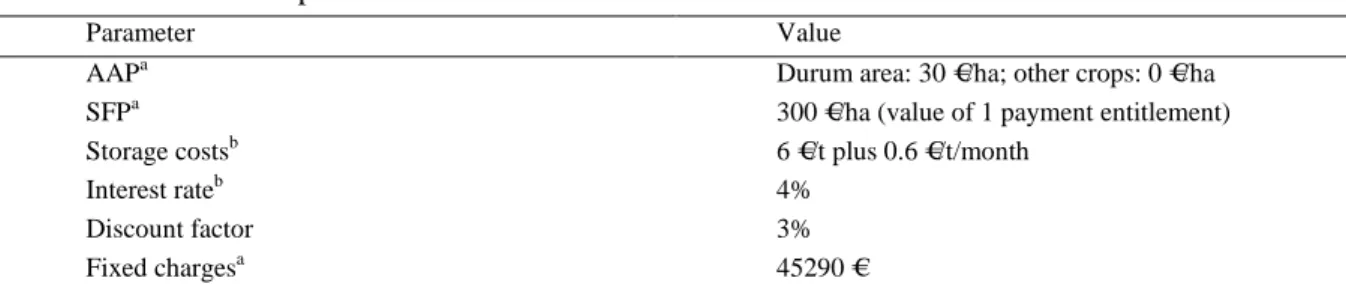
Table 2: Model parameters
Parameter Value
AAPa Durum area: 30 €/ha; other crops: 0 €/ha
SFPa 300 €/ha (value of 1 payment entitlement)
Storage costsb 6 €/t plus 0.6 €/t/month
Interest rateb 4%
Discount factor 3%
Fixed chargesa 45290 €
a
data provided by the regional extension service; b assumed at commercial rate.
4 RESULTS
In the simulations, we consider four levels of risk aversion: risk neutral (r=0), normally risk averse (r=0.5), rather risk averse (r=0.9), extremely risk averse (r=1.4)16. In the baseline scenario, the variability of price risk, in term of coefficient of variation (CV), corresponds to the one experienced during the period 1993-2006 and is represented by E=1 where E is the expansion factor. The value of one SFP is 300 € per payment entitlement (per ha).
We propose to test two scenarios on production and marketing decisions: an increase in the price risk and a decrease in the direct payments. In the first scenario, the price risk is firstly enhanced by 50% (E=1.5) and then by 100% (E=2). In the second scenario, the drop of the direct payment is realized by decreasing the SFP from 300 € (baseline scenario) to 150 €, by 50 €.
Furthermore, for each scenario, two cases are examined. A case where only pool contracts are supplied and a case where all marketing contracts are supplied. The comparison between both cases allows to evaluate the impact of supplying several marketing contract types on farm cropping decisions and thus to study the interactions between marketing and production decisions. Table 3 sum up the simulations realized.
Table 3: set experimental pattern
16 We followed the classification proposed by Hardaker et al. (2004). Yet, the values of the parameters are different from those given by the authors since we deal with the coefficient of relative risk aversion with respect to the income rather than with respect to wealth as in Hardaker et al.
14
Supply of pool contracts (case 1)
Supply of all contracts (case 2)
Scenario 0 (baseline) r=0 to 1.4 r=0 to 1.4
Scenario 1 r=0 to 1.4
price risk: +50% (E=1.5) price risk: +100% (E=2)
r=0 to 1.4
price risk: +50% (E=1.5) price risk: +100% (E=2)
Scenario 2 r=0 to 1.4 SFP varying from 300 to 150 €/ha r=0 to 1.4 SFP varying from 300 to 150 €/ha 4.1 Baseline scenario Case 1: supply of pool contracts only
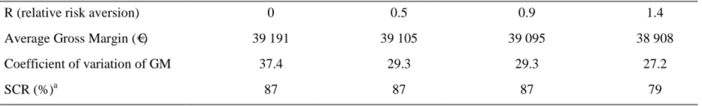
The results in Table 4 show that the degree of risk aversion influences the cropping plan. While the risk neutral farmer only uses the more profitable crops (see appendix 6.4), the risk averse farmers chooses to diversify the crop mix. Under positive risk aversion, durum wheat and soybean are partially replaced by soft wheat and sunflower, respectively. As it could be expected, when the level of risk aversion is increasing from normally to extremely risk averse, the area cultivated under low-input practice decreases since its induce a higher degree of riskiness. We calculated a Simulated Conversion Rate (SCR) defined as the rate of area cultivated under low-input practice over total cultivated area. A high value of SCR shows that the attractiveness of low-input practice as compared to conventional ones, whatever the level of risk aversion.
Case 2: supply of all marketing contracts
In the case 2, the farmer can choose to sell the production between pool contracts, storage contracts and forward contracts. When all these contracts are supplied to farmers, results are somewhat modified for “rather” and “extremely” risk averse farmers. First, it appears that storage contracts are the most adopted, followed by pool contracts. The adoption rate of pool contracts increases with the level of risk aversion since they enable to mitigate price risk. Forward contracts, which eliminate price risk, are never used, whatever the level of risk aversion in this baseline scenario.
The crop mix of the “rather” and “extremely” risk averse farmers is changed compared the case 1: less risky crops like conventional sunflower replace more risky ones like low-input rapeseed. Thus, it is observed that risk averse farmers prefer to use risky marketing contracts balanced by safer production choices (crops and practices). The result is a decrease of SCR when marketing contracts are introduced. This empirical result suggests dependence between marketing and production decisions.
15
Table 4: optimal farm plan under case 1 (pool contracts only)
R (relative risk aversion) 0 0.5 0.9 1.4
Average Gross Margin (€) 39 191 39 105 39 095 38 908
Coefficient of variation of GM 37.4 29.3 29.3 27.2
SCR (%)a 87 87 87 79
Optimal cropping plan (ha) Conventional practice: Soft wheat Durum wheat Dry corn Irrigated corn 14 14 14 14 Sunflower 0.2 8.6 Rapeseed Low-input practice: Soft wheat 25.05 32.8 31.7 Durum wheat 55.8 30.75 23 24.1 Dry corn 13.9 14 14 14 Irrigated corn Sunflower Rapeseed 23.3 23.2 23 14.6 a
Simulated Conversion rate
4.2 Scenarios testing the impact of increasing price risk and decreasing CAP subsidies
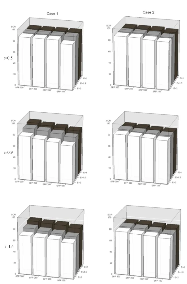
The scenarios are examined for the “normally”, the “rather” and the “extremely” risk averse farmers. We first compare case 1 (only pool contracts) with case 2 (all marketing contract types). It is observed in case 1 SCR decreases as the price risk increases and or that the SFP drops (Figure 1). The insurance effect (caused by higher price risk) and the wealth effect (due to lower direct payments) induce the adoption of less risky farming practices. Moreover, the Figure 1 shows that the higher the level of risk aversion, the larger the insurance and the wealth effects. In case 2, the SCR stays the same for any level of riskiness and for any level of SFP since the insurance and wealth effects have no more impact on cropping choices. This result might be due to the presence of different marketing alternatives which contributes to stabilize production choices. As shown in Figure 2, insurance and wealth effects act rather on marketing decisions than on production decisions. Indeed, they contribute to decrease the proportion of the production stored and to enhance the part under pool contracts. We observe that, if the drop of SFP is combined with a higher price risk, forward contracting is used for very small quantities only.
16
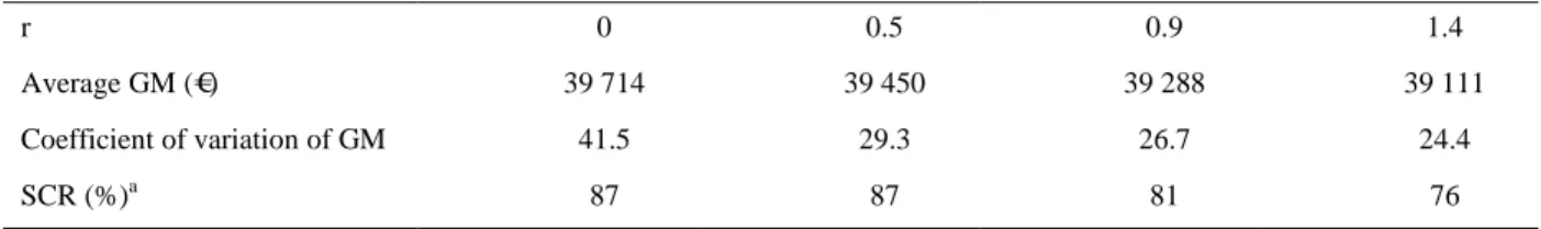
Table 5: optimal farm plan and marketing contract choices under case 2 (all the marketing contracts)
r 0 0.5 0.9 1.4
Average GM (€) 39 714 39 450 39 288 39 111
Coefficient of variation of GM 41.5 29.3 26.7 24.4
SCR (%)a 87 87 81 76
Optimal cropping plan (ha) Conventional practice: Soft wheat Durum wheat Dry corn Irrigated corn 14 14 14 14 Sunflower 5.8 11.5 Rapeseed Low-input practice: Soft wheat 25.35 29.2 30.3 Durum wheat 55.8 30.45 26.6 25.5 Dry corn 13.9 14 14 14 Irrigated corn Sunflower Rapeseed 23.3 23.2 17.4 11.7
Optimal marketing contract choices (%)a
Pool contract 37 43 45
Storage contract 100 63 57 55
Forward contract
17
Figure 1: Effect of an increase of the price risk and a decrease of direct payments on the SCR under the 2 cases and for 3 levels of risk aversion: r=0.5 (top); r=0.9 (middle); r=1.4 (low).
r=0.5
r=0.9
19
5 DISCUSSION AND CONCLUSION
The analytical model developed in section 2 sheds light on the conditions under which production decisions are separable from marketing decisions, risk aversion and risk perception. We have shown that these conditions are rather restrictive, even when it is assume that hedging is perfect (presence of price risk only). This advocate for the relevance of taking care of marketing decisions when agricultural economists study the impact of agricultural policies on farm adjustments. We also showed that insurance effect and wealth effect influence marketing contract choices, even though the effects are contract-specific. For example, a drop of direct payments increases the demand for forward contract and reduces the demand for storage through a wealth effect.
To illustrate our analytical results, we built a MP farm model applied to a representative farm of Midi-Pyrénées Region. Firstly, we have shown that price risk and direct payments affect both production and marketing choices. The latter choices are revealed to be important adjustment tools with the proportion of storage contracts and pool contracts that vary when farmers have to cope with policy changes. Pool contract seems the appropriate marketing strategy to mitigate the price risk in the actual economic environment. Indeed, even in the case of strong risk aversion, forward contracts are few used by farmers in our simulation, even if their use is enhanced when price risk is sharper and direct payments lower. All these results are consistent with empirical findings showing that government policies tend to reduce the demand for hedging (Woolverton and Sykuta, 2009) and that in an income-support economic environment, risk averse farmers are more likely to use pool contracts rather than forward contracts (Ricome, 2012). Secondly, by comparing in our simulations a case where only pool contracts are supplied to a case where three contract types are supplied in a changing economic environment, we addressed the issue of the interactions between production decisions, marketing decisions and government policies. We observed that a large supply of marketing contracts allows to stabilize production choices. In particular, we found that marketing contracts can contribute to help farmers to adopt green practices, which are riskier than conventional techniques intensive in chemical inputs. Our simulation results also question the real impact of direct payment, through the wealth effect, on production decisions. The weak impact of wealth effect on production decisions has already been pointed out in empirical ex post analysis (Bhaskar and Beghin, 2007). To figure out this gap between the theory and the empirical observations, several arguments have been suggested. It could be due to (i) the weak share of direct payments over the total revenue of the farmer (Sckokai and Antón, 2005); (ii) the impact of direct payments on input use that affect in turn production risk (Serra et al., 2006); (iii) the effect of direct payments on land value that make the landowner the final beneficiary rather than the farmer (Femenia et al., 2009). But the results obtained here lead to suggest another hypothesis: the direct payment may first lead to marketing adjustments so that production adjustments are marginal. Even if it has not been explicitly taken into account in the MP model, this proposition could also come from the presence of agronomic and technical rigidities on production sides that do not exist on marketing side. This could be an interesting scope for further research.
20
REFERENCES
Abadi Ghadim, A. K. and D. J. Pannell (1999). A conceptual framework of adoption of an agricultural innovation. Agricultural Economics 21(2): 145-154.
Agreste (2009). Ministère de l'agriculture, de l'alimentation, de la pêche, de la ruralité et de l'aménagement du territoire.http://www.agreste.agriculture.gouv.fr/page-d-accueil/article/donnees-en-ligne.
Anderson, R. W. and J. P. Danthine (1983). Hedger diversity in futures markets. The Economic Journal 93: 370-389.
Bhaskar, A. and J. C. Beghin (2007). How coupled are decoupled farm payments? A review of coupling mechanisms and the evidence. Departement of economics working papers series, Iowa State University: 37 p.
Brorsen, B. W. (1995). Optimal hedge ratios with risk-neutral producers and nonlinear borrowing costs. American Journal of Agricultural Economics 77(1): 174-181.
Coble, K. H., J. C. Miller, M. Zuniga and R. Heifner (2004). The joint effect of government crop insurance and loan programmes on the demand for futures hedging. European Review of Agricultural Economics 31(3): 309-330.
Coop de France (2010). La collecte des céréales, oléagineux, et protéagineux, l'approvisionnement, la transformation.http://www.coopdefrance.coop/sites/FFCAT/default.aspx
Dalal, A. J. and M. Alghalith (2009). Production decisions under joint price and production uncertainty. European Journal of Operational Research 197(1): 84-92.
Danthine, J. P. (1978). Information, futures prices, and stabilizing speculation. Journal of Economic Theory 17(1): 79-98.
Di Falco, S. and J. P. Chavas (2006). Crop genetic diversity, farm productivity and the management of environmental risk in rainfed agriculture. European Review of Agricultural Economics 33(3): 289.
European Commission (2011). The future of CAP direct payments. Agricultural policy perspectives briefs, Brief 2.
Feder, G., R. E. Just and D. Zilberman (1985). Adoption of agricultural innovations in developing countries: A survey. Economic Development and Cultural Change 33(2): 255-298.
Feder, G., Just, R. E., Schmitz, A. (1980). Futures markets and the theory of the firm under price uncertainty. The Quarterly Journal of Economics 94(2): 317-328.
Femenia, F., A. Gohin and A. Carpentier (2010). The Decoupling of Farm Programs: Revisiting the Wealth Effect. American Journal of Agricultural Economics 92(3): 836-848.
Grant, D. (1985). Theory of the firm with joint price and output risk and a forward market. American Journal of Agricultural Economics 67(3): 630-635.
Harwood, J., R. Heifner, K. H. Coble, J. Perry and A. Somwaru, (eds.) (1999). Managing Risk in Farming: Concepts, Research, and Analysis. Agricultual Economic Reports No. 774. Washington D.C., U.S. Department of Agriculture.
Hennessy, D. A. (1998). The production effects of agricultural income support policies under uncertainty. American Journal of Agricultural Economics 80(1): 46-58.
Holthausen, D. M. (1979). Hedging and the competitive firm under price uncertainty. The American Economic Review 69(5): 989-995.
Just, R. E. and Q. Weninger (1999). Are crop yields normally distributed? American Journal of Agricultural Economics 81: 287-304.
Lapan, H. and G. Moschini (1994). Futures hedging under price, basis, and production risk. American Journal of Agricultural Economics 76(3): 465-477.
Lapan, H., G. Moschini and S. D. Hanson (1991). Production, hedging, and speculative decisions with options and futures markets. American Journal of Agricultural Economics 73(1): 66-74.
Lien, G. and J. B. Hardaker (2001). Whole-farm planning under uncertainty: impacts of subsidy scheme and utility function on portfolio choice in Norwegian agriculture. European Review of Agricultural Economics 28(1): 17-36.
21
Lien, G., J. B. Hardaker, M. van Asseldonk and J. W. Richardson (2009). Risk programming analysis with imperfect information. Annals of Operations Research: 1-13.
Losq, E. (1982). Hedging with price and output uncertainty. Economics Letters 10(1-2): 65-70.
Mosnier, C., A. Ridier, C. Kephaliacos and F. Carpy-Goulard (2009). Economic and environmental impact of the CAP mid-term review on arable crop farming in South-western France. Ecological Economics 68(5): 1408-1416.
Pannell, D., G. Hailu, A. Weersink and A. Burt (2008). More reasons why farmers have so little interest in futures markets. Agricultural Economics 39(1): 41-50.
Richardson, J. W., S. L. Klose and A. W. Gray (2000). An applied procedure for estimating and simulating multivariate empirical (MVE) probability distributions in farm-level risk assessment and policy analysis. Journal of Agricultural and Applied Economics 32(2): 299-316.
Ricome, A. (2012). Analyse économique des décisions de commercialisation et de production des explitants agricoles exposés à la volatilité des prix. Application au secteur des grandes cultures en Midi-Pyrénées. Thèse de doctorat, Université de Toulouse 1, 317 p.
Ridier, A., M. El Ghali, C. Képhaliacos and G. Nguyen (2011). The impact of labor constraint and policy incentives on the adoption of low input practices under yield risk supported bt the CAP green payments in cash crop farms.
Sandmo, A. (1971). On the theory of the competitive firm under price uncertainty. The American Economic Review 61(1): 65-73.
Sckokai, P. and J. Antón (2005). The degree of decoupling of area payments for arable crops in the European Union. American Journal of Agricultural Economics 87(5): 1220-1228.
Serra, T., D. Zilberman, B. K. Goodwin and A. Featherstone (2006). Effects of decoupling on the mean and variability of output. European Review of Agricultural Economics 33(3): 269-288.
Uri, N. (2000). An evaluation of the economic benefits and costs of conservation tillage. Environmental Geology 39(3): 238-248.
Viaene, J. M. and I. Zilcha (1998). The behavior of competitive exporting firms under multiple uncertainty. International Economic Review 39(3): 591-609.
Wang, H. H., L. D. Makus and X. Chen (2004). The impact of US commodity programmes on hedging in the presence of crop insurance. European Review of Agricultural Economics 31(3): 331-352.
Woolverton, A. E. and M. E. Sykuta (2009). Do Income Support Programs Impact Producer Hedging Decisions? Evidence from a Cross-Country Comparative. Applied Economic Perspectives and Policy 31(4): 834-852.
APPENDIX
A: Marketing contracts in the French cash crop sector
In France, it is mandatory for grain farmers to sell their production exclusively to an officially authorized grain retailer. Two kinds of status exist: cooperative groups, i.e groups owned by farmers, and groups owned by families or investors. Currently, the 200 French grain cooperative groups collect 75% of the total grain production (Coop de France, 2010) and hold a central position in the grain industry. They propose to their members different pricing mechanisms through marketing contracts.
French co-ops used to supply a unique pricing arrangement, a pool contract. In such a price-setting system, the producer is required to deliver grain at harvest and the quantity is priced at the average sale price achieved by the co-op. The first amount paid, which occurs just after the harvest, is determined by the co-op’s forecast of the expected average price (minus the co-op’s administrative cost). At the end of the marketing campaign, if the actual average sale price is higher than the forecast price, a price complement is paid to farmers. Therefore, a pooling contract reduces the price risk
22
because the farmer is paid an average price (the intra-annual price risk is smoothed) and is protected against downward price movements while still having the opportunity to benefit from upward price fluctuations. In the static analytical framework presented above, the pool contract can be seen as the cash-at-harvest contract. Since the mid-2000’s, other marketing contracts have been developed on the French market, that are better tailored to different categories of farmers than a unique pool contracts. Even if details about the contractual structure may vary, two other main contracts are now used by French arable farmers: storage contract and forward contract (Ricome, 2012).
Our model into account three dimension of a marketing contract: the average price, the price risk level and the date(s) of payment. Marketing choices will then be influenced by price enhancement, risk, and cash flow considerations. Table 1 gives the main contractual attributes for each of those contracts.
Table 1: Attributes of marketing contracts
Average price Price risk exposure Effect on cash flow constrainta
Pool contract Medium Medium Medium
Storage contract Strong Strong Strong
Forwarding contract
Weak Weak Weak
a
The earlier and the higher the payment, the less the effect on the cash-flow constraint.
Since a pool contract corresponds to an average annual price, the degree of price risk exposure under this contract is weaker than under a storage strategy but stronger than under a forwarding contract in which the price is fixed before harvest. As a counterpart, it is expected a higher average price from storage and a lower one from the forward contracting. The payment under a forwarding contract occurs at harvest while the average price from a pool contract is paid in two stages, a few weeks after the harvest (in the model we assume that 70%% of the price is paid at the first stage) and at the end of the marketing campaign (the 30% left over). Effects of these two contracts on the farm’s cash flow constraint are then slightly different.
B: Proofs related to the proposition 1
Proofs are based on the article of Sandmo (1971). Since the proof for ∗ can be found there, we will focus here on the proofs related to ∗ and ∗.
Proof that /)/‰{ 0 :
From expression (14B), we know that xŠ‡Q)Q‰ xŠ‡ W! RS‹ RXRŒ
|•‹|Y. Because /)/‰/SŽ #′′ ! (A1)
And given that |•Ž| P 0 from the second-order condition, we only have to show that (A1) is non-positive. Let be the profit when E . Because the farmer is DARA, we have:
E • ⇔ • ⇒ “ !8
99 :
89 : { “ (A2) Moreover, for • , we have !#′ ! • 0 (A3)
23 Multiplying (A2) by (A3), we obtain:
#22 ! { ! “ €F #2 ! ∀ E
Take expectations of both sides yields:
1#22 ! 3 { !
“ 1#2 ! 3 0 (A4)
Where the last equality is implied by (2b). we thus have proved the wealth effect on the forward demand.
Proof that /‰/ • 0 :
From expression (14C), we know that xŠ‡ >Q‰Q ? xŠ‡ W! R²‹ RIRŒ
|•‹|Y. Because / /‰/SŽ #′′ ! ! (A5)
And given that |•Ž| P 0 from the second-order condition, we only have to show that (A4) is non-negative. Let be the profit when ! . Because the farmer is DARA, we have:
! • ⇔ • ⇒ “ !8
99 :
89 : { “ (A6) Moreover, for ! • , we have !#′ ! ! { 0 (A7) Multiplying (A6) by (A7), we obtain:
#22 ! ! • !“ #2 ! ! ∀E, E
Take expectations of both sides yields:
1#22 ! ! 3 • !“ 1#2 ! ! 3 0
Where the last equality is implied by expression (2c). We thus have proved the presence of a wealth effect on contract’s demands.
Complement on the proof of the proposition 1:
Given that the coefficient of relative risk aversion h “ , it can be also shown
following the same steps that for a producer IRRA: 1#22 ! 3 • 0 (A8)
For a producer CRRA we have: 1#22 ! 3 0 (A9)
These results are useful for the proof of the proposition 2.
C: Proofs related to the proposition 2
Proofs are based on the article of Dalal and Alghalith (2009). We will give here the proofs related to the effects of on ∗. The proofs related to on ∗ and related to ∗ and ∗ follow immediately.
Proof that /–/)
<• 0. Using expression (14B), we get:
/) /–< ! RS‹ RXR—< |•‹| ! e |•‹|˜ 1# 22 € ∗! ∗! ∗ ̃ ! 3 ! 1#2 € ̃ 3™ (A10)
24 Given that ! e
|•‹|• 0, we have to sign 1#
22 € ∗! ∗! ∗ ̃ ! 3 ! 1#2 € ̃ 3.
Let first sign 1#22 € ∗! ∗! ∗ ̃ ! 3 :
We know that ̃ ∗! ∗! ∗ ! ! •, which can be
developed as follow: ̃ ∗! ∗! ∗
Thus : ̃ ∗! ∗! ∗ –e
< ! . It can then be write:
1#22 ∗! ∗! ∗ ̃ ! 3 1 1#22 ! ! 3
1
1#22 ! 3 ! 1 1#22 ! 3
From the proof given above (A8 and A9), we know that the first term is positive (null) for a IRRA (CRRA) farmer. Furthermore, the second term is negative for DARA farmer (A4). We thus have for a DARA-IRRA or DARA-CRRA17: 1#22 € ∗! ∗! ∗ ̃ ! 3 • 0
Let now sign 1#2 € ̃ 3. We know that:
1#2 ̃ 3 š#2 ! › 1 BC1#2 , 3 { 0
Thus, we have proved that /–/)
<• 0 if the producer is DARA-CRRA or DARA-IRRA.
17
25
D: Average, coefficient of variation and skewness of alternative’s gross margins (Table 6)
crop technique Marketing
contract Average GM (€) CV of GM1 Skewness of GM2
Soft wheat Conventio
nal K1 408 31.6 0.26 K2A 423 29.6 0.15 K2B 408 35.8 0.2 K3 371 19.1 -0.35 Low-input K1 423 38.7 0.12 K2A 436 37.6 0.06 K2B 421 41 0.24 K3 393 36.6 -0.89
Durum wheat Conventio
nal K1 389 28.7 0.25 K2A 410 32.7 0.54 K2B 402 31.6 0.5 K3 362 25.1 -0.35 Low-input K1 427 38 -0.27 K2A 445 39.3 0.06 K2B 438 39.2 0.01 K3 406 38.7 -0.89
Dry corn Conventio
nal K1 308 57.7 0.49 K2A 327 60.9 0.56 K2B 350 58.5 0.76 K3 280 28.5 -0.72 Low-input K1 334 7.1 0.09 K2A 353 73.9 0.2 K2B 375 71.1 0.31 K3 305 55.3 -0.91
Irrigated corn Conventio
nal K1 784 37.3 0.43 K2A 822 40.2 0.51 K2B 865 39.7 0.74 K3 736 13.9 -0.93 Low-input K1 717 53.2 0.02 K2A 754 55.4 0.12 K2B 793 54.2 0.25 K3 669 38.7 -1.01 sunflower Conventio nal K1 286 31.9 0.6 K2A 300 40.6 0.74 K2B 284 38.1 0.63 K3 258 22.6 -0.09 Low-input K1 268 48.3 -0.09 K2A 280 53.8 0.29 K2B 265 52.9 0.18 K3 241 44.4 -0.63 Rapeseed Conventio nal K1 285 46.2 -0.21 K2A 299 47.5 -0.16 K2B 309 48.8 0.23 K3 240 46.9 -0.84 Low-input K1 303 66.6 -0.59 K2A 315 66.7 -0.49 K2B 324 67.1 -0.3 K3 263 71.3 -0.93 1