HAL Id: hal-03087340
https://hal.inrae.fr/hal-03087340
Submitted on 23 Dec 2020
HAL is a multi-disciplinary open access
archive for the deposit and dissemination of
sci-entific research documents, whether they are
pub-lished or not. The documents may come from
teaching and research institutions in France or
abroad, or from public or private research centers.
L’archive ouverte pluridisciplinaire HAL, est
destinée au dépôt et à la diffusion de documents
scientifiques de niveau recherche, publiés ou non,
émanant des établissements d’enseignement et de
recherche français ou étrangers, des laboratoires
publics ou privés.
Lessons learnt from a blind test
Daniela Molinari, Anna Rita Scorzini, Chiara Arrighi, Francesca Carisi, Fabio
Castelli, Alessio Domeneghetti, Alice Gallazzi, Marta Galliani, Frédéric
Grelot, Patric Kellermann, et al.
To cite this version:
Daniela Molinari, Anna Rita Scorzini, Chiara Arrighi, Francesca Carisi, Fabio Castelli, et al.. Are
flood damage models converging to “reality”? Lessons learnt from a blind test. Natural Hazards and
Earth System Sciences, European Geosciences Union, 2020, 20 (11), pp.2997-3017.
�10.5194/nhess-20-2997-2020�. �hal-03087340�
https://doi.org/10.5194/nhess-20-2997-2020 © Author(s) 2020. This work is distributed under the Creative Commons Attribution 4.0 License.
Are flood damage models converging to “reality”?
Lessons learnt from a blind test
Daniela Molinari1, Anna Rita Scorzini2, Chiara Arrighi3, Francesca Carisi4, Fabio Castelli3, Alessio Domeneghetti4, Alice Gallazzi1, Marta Galliani1, Frédéric Grelot5, Patric Kellermann6, Heidi Kreibich6, Guilherme S. Mohor7, Markus Mosimann8, Stephanie Natho7, Claire Richert5, Kai Schroeter6, Annegret H. Thieken7,
Andreas Paul Zischg8, and Francesco Ballio1
1Department of Civil and Environmental Engineering, Politecnico di Milano,
Piazza Leonardo da Vinci 32, 20133 Milan, Italy
2Department of Civil, Environmental and Architectural Engineering,
University of L’Aquila, Via Gronchi 18, 67100 L’Aquila, Italy
3Department of Civil and Environmental Engineering, University of Florence, Piazza San Marco 4, 50121 Florence, Italy 4Department of Civil, Chemical, Environmental and Material Engineering,
University of Bologna, Viale Risorgimento 2, 40136 Bologna, Italy
5G-EAU, Univ Montpellier, AgroParisTech, CIRAD, IRD, INRAE, Montpellier SupAgro, Montpellier, France 6GFZ German Research Centre for Geosciences, Section Hydrology, Telegrafenberg, 14473 Potsdam, Germany 7Institute of Environmental Science and Geography, University of Potsdam,
Karl-Liebknecht-Strasse 24–25, 14476 Potsdam, Germany
8Institute of Geography, Mobiliar Lab for Natural Risks, Oeschger Centre for Climate Change Research,
University of Bern, Hallerstrasse 12, 3012 Bern, Switzerland
Correspondence: Daniela Molinari ([email protected]), and Anna Rita Scorzini ([email protected]) Received: 7 February 2020 – Discussion started: 24 February 2020
Revised: 7 September 2020 – Accepted: 2 October 2020 – Published: 9 November 2020
Abstract. Effective flood risk management requires a realis-tic estimation of flood losses. However, available flood dam-age estimates are still characterized by significant levels of uncertainty, questioning the capacity of flood damage mod-els to depict real damages. With a joint effort of eight inter-national research groups, the objective of this study was to compare, in a blind-validation test, the performances of dif-ferent models for the assessment of the direct flood damage to the residential sector at the building level (i.e. microscale). The test consisted of a common flood case study character-ized by high availability of hazard and building data but with undisclosed information on observed losses in the implemen-tation stage of the models. The nine selected models were chosen in order to guarantee a good mastery of the models by the research teams, variety of the modelling approaches, and heterogeneity of the original calibration context in rela-tion to both hazard and vulnerability features. By avoiding possible biases in model implementation, this blind
compar-ison provided more objective insights on the transferability of the models and on the reliability of their estimations, es-pecially regarding the potentials of local and multivariable models. From another perspective, the exercise allowed us to increase awareness of strengths and limits of flood damage modelling, which are summarized in the paper in the form of take-home messages from a modeller’s perspective.
1 Introduction
Efficient and effective flood risk management requires a re-alistic estimation of flood losses, implying the use of reli-able models for flood hazard, damage, and risk assessment (Meyer et al., 2013; Gerl et al., 2016; Zischg et al., 2018; Wagenaar et al., 2018; Molinari et al., 2019). Although sev-eral hydraulic models are available (Teng et al., 2017), their variety seems to be overtopped by the variety of flood
dam-age models as, according to Gerl et al. (2016), 28 models (including 652 functions) exist in Europe alone to assess flood losses, whereas almost half of them focus on residential buildings.
Even within the residential sector and with respect to di-rect damage (i.e. damage due to the didi-rect contact with the flooding water), the diversity of approaches is manifold. First, the models are classified according to the intended spa-tial scale of the analysis: while microscale models refer to the individual exposed building, mesoscale models work at more aggregated scales, like land use or administrative units, with large-scale spatial units (like regions or countries) being at the base of macroscale models (Merz et al., 2010).
A second difference lies in the approach adopted for model development, with empirical models using damage data col-lected after flood events (e.g. Merz et al., 2004) and synthetic approaches implementing information collected via what-if questions (e.g. Penning-Rowsell et al., 2005). Still, both cat-egories are characterized by a variety of methods; for ex-ample, empirical data can be interpreted by means of dif-ferent statistical and mathematical tools ranging from sim-ple regression (e.g. Merz et al., 2004) to more sophisticated machine-learning algorithms and data-mining approaches (e.g. Merz et al., 2013; Amadio et al., 2019). A distinc-tion can also be made between absolute- and relative-damage models: the first directly return a value in a specific currency (Dottori et al., 2016; Rouchon et al., 2018), while relative-damage models estimate the physical vulnerability or the degree of loss of an exposed asset (Fuchs et al., 2019a) to be multiplied by its monetary value to assess the damage. Linked to this point is the question of what is defined as ex-posure in the models: besides the distinction of whether a model relies on the value of the whole building or just of the affected floors, it is also important to know whether, for instance, the basement is considered as well. Moreover, ex-posure assessment may differ regarding the monetary value and whether it is based on e.g. market or replacement values (Röthlisberger et al., 2018) rather than full replacement costs or depreciated values (Merz et al., 2010).
A final important difference among the models lies in the number and type of considered input parameters, i.e. on model complexity. The simplest damage models (referred to in the following as “low-variable models”) take into account a small number of variables, mostly the water depth at the building location as well as building area and its monetary value (only in the case of relative models). Even in their sim-plicity, these models can significantly differ from each other due to the distinct shapes of the underlying damage func-tions, e.g. square root function (Dutta et al., 2003; Carisi et al., 2018), beta distribution function (Fuchs et al., 2019b), or graduated function (Jonkman et al., 2008; Arrighi et al., 2018a). In contrast, multivariable models consider numerous hazard as well as exposure and vulnerability input factors and, consequently, are supposed to be more accurate when detailed data are available (Thieken et al., 2008; Schröter
et al., 2014; Wagenaar et al., 2017; Amadio et al., 2019). Nevertheless, simple models tend to be the most widely used due to their ease of implementation and low requirements for input data. Hence, flood damage modellers always have to envisage the trade-off in the model choice, i.e. using a com-plex, probably more accurate model with specific data re-quirements or a simple, probably less accurate one that can be applied without extensively available data. However, it has been shown that even a small ensemble of models out-performs individual models, with the additional advantage of providing uncertainty information (Figueiredo et al., 2018).
What most models have in common is that they are cali-brated in specific contexts, usually representative of a certain spatially limited region. In many cases, instead, validation of flood damage models is lacking (Merz et al., 2010; Gerl et al., 2016; Molinari et al., 2019). Where it is not lacking, the data used for model validation are often either a subset of the dataset used for calibration or are collected in the same region or country of model development. This implies that, even if a model has been locally validated, it is not necessar-ily correct to apply it to any other region unless this region reflects the context for which the model was derived. For in-stance, the application of a damage model that has been de-veloped for alpine areas (i.e. house-building tradition of the European Alps and flood processes involving significant sed-iment transport) to a coastal country like the Netherlands, and vice versa, is prone to lead to large discrepancies from real-ity (e.g. Cammerer et al., 2013). Hence, flood damage models need to be tested in regions other than those where they were calibrated in to be confident of their transferability in space.
Nevertheless, what all models and modellers deal with is the lack of data for model calibration and validation (Merz et al., 2010; Jongman et al., 2012; Meyer et al., 2013; Moli-nari et al., 2019). The overall economic impact of a flood is hardly reproduced by ex-post data, and then biases also have to be taken into account when transferring models to different regions, e.g. due to different insurance conditions, uncom-pleted claims, etc. Moreover, even years after flood events, monetary losses can be revised due to long-term recovery. As an example, monetary losses of the 2013 flood in Ger-many were estimated at EUR 6.7 million in 2013 (Deutscher Bundestag, 2013) and changed over the following years to EUR 8.2 million (Bundesministerium für Verkehr und digi-tale Infrastruktur, 2016). For this reason, comparative stud-ies over a broad range of test cases (i.e. different validation datasets) are essential for acquiring a thorough understanding of the performances of the modelling tools that could help in enhancing the confidence in their reliability.
The aim of this study is to contribute to the understanding of models’ transferability and reliability by testing and com-paring different damage models in a blind-validation test. This joint effort of eight international research groups con-sists of a common flood case study characterized by high availability of hazard and building data but with undisclosed information on observed losses in the implementation stage
of the models. Tested models have been chosen among those mastered by the authors; indeed, the authors were either de-velopers of the models or experienced users with significant knowledge of them in order to prevent any possible bias in the results that could arise from an incorrect application of the models (for example, a non-expert user may misunder-stand the meaning of some input variables, which would af-fect the final estimation).
Even though comparative analyses on the performance of damage models have become more frequent in the litera-ture (Jongman et al., 2012; Cammerer et al., 2013; Scorzini and Frank, 2017; Carisi et al., 2018; Figueiredo et al., 2018; Amadio et al., 2019), according to the authors’ knowledge, this study would represent the first flood damage model com-parison performed in a blind mode. This type of comcom-parison can provide more objective insights for a better understand-ing of models’ capabilities and then for reducunderstand-ing modellunderstand-ing uncertainties, as already demonstrated in similar tests per-formed for other disciplines like seismology, hydrology, and computational fluid dynamics (Smith et al., 2004; Soares-Frazao et al., 2012; Krogstad and Eriksen, 2013; Zelt et al., 2013; Andreani et al., 2019; Ransley et al., 2019; Skorek et al., 2019). Indeed, possible biases are avoided as partic-ipants cannot be influenced by validation data, these data be-ing undisclosed in the implementation phase of the models, e.g. by trying to adjust or tune their models, especially re-garding the more qualitative input parameters, in light of ob-served damages.
This study focuses on microscale (i.e. individual item scale) direct damage assessment to residential buildings, in line with the larger availability of damage modelling ap-proaches developed in Europe for this specific sector and scale.
As the research groups use approaches representing many different types and characteristics of models (low-variable – multivariable; absolute – relative; graduated – regression – machine learning – synthetic), being calibrated on the basis of observed data stemming from different countries (Austria, France, Germany, Italy, Japan, Netherlands) with different landscapes and levels of complexity in exposure and vulner-ability, the blind test as performed in this study can provide an in-depth understanding of the links between model fea-tures, their transferability, and the reliability of the estimated damages.
In particular, the blind test allowed us to investigate these specific questions raised from the evidence supplied by the literature (Thieken et al., 2008; Cammerer et al., 2013; Schröter et al., 2014; Dottori et al., 2016; Wagenaar et al., 2017; Amadio et al., 2019): do local models (i.e. models cal-ibrated with data from a context similar to the investigated one) outperform other models? Do multivariable models per-form better than the simplest ones, and if so, why?
The paper is organized as follows. The methodology, mod-els, and case study implemented in the blind test are first presented in Sect. 2. Section 3 discusses results of the test,
first by considering damage estimates obtained in a blind im-plementation of the models and then by comparing damage estimates with documented losses. Answers to the specific research questions are provided in Sect. 4. Finally, in Sect. 5, evidence from the blind test is synthesized in lessons learnt (on flood damage modelling) from a modeller’s perspective, including the identification of research needs for further im-provements of flood damage models.
2 The blind test: case study, methodology, models The main idea behind the blind test was to evaluate the per-formance of different flood damage models by their imple-mentation to a common case study to obtain enhanced infor-mation on their transferability, validity, and reliability; the test is defined as “blind” as, in order to avoid bias in the estimation process, the value of the observed damage was unknown to modellers in the implementation stage of the models. In particular, damage data were unblinded only to one group, which was the promoter of the initiative and re-sponsible for data and results management. All input data required to reproduce the damage scenario for the examined event were made available to the participants, who were then asked to submit their results to the exercise manager in an es-tablished time frame. Once all contributions from the differ-ent groups had been gathered, observed data were disclosed, and models’ performances were compared and analysed in a shared discussion between the participants.
2.1 Case study
The investigated context is the town of Lodi, northern Italy (Fig. 1), which was hit by a severe flood on 25–26 Novem-ber 2002 caused by the overflow of the Adda river as a result of 2 weeks of heavy rainfalls over north-western Italy.
The flood caused severe damage to residential buildings, commercial activities, and public services in the area, includ-ing the main hospital. Fortunately, no fatalities occurred. The event was chosen as reference for the exercise as it is well documented and characterized by a high availability of haz-ard, exposure, and vulnerability data. In detail, with respect to the hazard, information on observed water depths was available for more than 260 points within the inundated area, deriving from indications provided by municipal technicians and by citizens in damage compensation requests as well as from interpretation of photographs taken during or immedi-ately after the flood. These data were used for the validation of the 2-D hydraulic simulation of the event: the resulting av-erage absolute differences between observed and calculated water depths within the inundated area ranged from 0.2 to 0.4 m, depending on the validation zone in which observed water depth data were aggregated (Scorzini et al., 2018). This is surely a possible source of uncertainty; however, reported differences could be considered to provide relatively small
Figure 1. Map of the flooded area and affected buildings (background map from Esri, DigitalGlobe, GeoEye, Earthstar Geographics, CNES/Airbus DS, USDA, USGS, AeroGRID, IGN, and the GIS user community).
impacts on the damage estimation. Moreover, given that all tested damage model shared the same hazard data, this would be a common source of uncertainty that should not affect the overall results of the blind test. Available microscale data on exposure and vulnerability of residential buildings are shown in Table 1.
Altogether, observed damage was known for 345 of the 877 buildings in the flooded area (after hydraulic simulation; Fig. 1), as derived from claims compiled by citizens after the flood to ask for public compensation. Claims were mostly collected by the Municipality of Lodi and, in small part, by the regional authority of the Lombardy region after the event. Available claims data, in their original paper form, were then acquired and successively stored in a georeferenced digital database by a team of researchers of Politecnico di Milano in summer 2017. As regards data from the municipality, origi-nal claims were organized in forms, including information on the owner, the address of the flooded building, its typology (e.g. apartment, single house), the number of affected floors,
a description of the physical damage, and its translation into monetary terms (distinguishing for the different rooms of the building among damage to walls, windows and doors, floors, systems, and content). In few cases, information on water depth inside the building and on clean-up costs, non-usability of the building, and intangible damage (e.g. loss of memora-bilia) was also inferred from the qualitative damage descrip-tion in the forms. The quality and reliability of data included in the claims was not uniform since only some of the owners justified the costs for fixing damage by means of invoices. As regards data from the secondary source (i.e. the regional au-thority), they included limited information on the owner, the address of the flooded building, and the monetary value of the damage, distinguished between damage to structure and contents.
2.2 Methodology
The methodological approach followed in the test included the following steps.
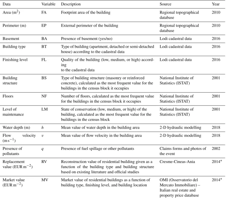
Table 1. Available microscale data for the blind exercise.
Data Variable Description Source Year
Area (m2) FA Footprint area of the building Regional topographical
database
2010
Perimeter (m) EP External perimeter of the building Regional topographical
database
2010
Basement BA Presence of basement (yes/no) Lodi cadastral data 2016
Building type BT Type of building (apartment, detached or semi-detached
house) according to the cadastral data
Lodi cadastral data 2016
Finishing level FL Quality of the building (low, medium, or high)
accord-ing
to the cadastral data
Lodi cadastral data 2016
Building structure
BS Type of building structure (masonry or reinforced concrete), calculated as the most frequent value for the buildings in the census block it occupies
National Institute of Statistics (ISTAT)
2001
Floors NF Number of floors, calculated as the most frequent value
for the buildings in the census block it occupies
National Institute of Statistics (ISTAT)
2001
Level of maintenance
LM State of conservation (low, medium, or high) of the building, calculated as the most frequent value for the buildings in the census block
National Institute of Statistics (ISTAT)
2001
Water depth (m) h Mean value of water depth in the building area 2-D hydraulic modelling 2018
Flow velocity
(m s−1)
v Mean value of flow velocity in the building area 2-D hydraulic modelling 2018
Presence of pollutants
q Presence of fuel spillage or other pollutants Claims forms and photos of
the event
2002
Replacement value (EUR m−2)
RV Reconstruction value of residential building given as a function of the building type and building structure based on existing literature and official studies
Cresme-Cineas-Ania 2014∗
Market value (EUR m−2)
MV Market value of residential buildings as a function of building type, finishing level, and building location
OMI (Osservatorio del Mercato Immobiliare) – Italian real estate and property price database
2014∗
∗For the objective of the exercise, data were discounted to 2002 values.
– Step 1: identification of damage models to be tested. The choice was based on several considerations: (i) good mastery of the models by the research team (i.e. dam-age models regularly used or initially developed by the groups); (ii) heterogeneity of the approaches by consid-ering simple and multivariable models, empirical and synthetic approaches, and absolute and relative models; and (iii) models being calibrated in a different context than the investigated one. The choice converged to the nine models described in Sect. 2.3.
– Step 2: implementation of the models to the case study in a blind mode. The models were implemented inde-pendently by the research groups (i.e. each group ap-plied one to three models according to its specific
exper-tise) to calculate damage to all 877 buildings that were exposed to the 2002 Lodi flood according to the inun-dation area simulated by the hydraulic model (Scorzini et al., 2018). All the groups used available and common data on hazard, exposure, and vulnerability, as described in Table 1. While this step was simple for Italian mod-els (which were originally developed to work with the same kind of data available for the case study), some efforts were required for the other models, particularly in the case of multivariable ones. This is due to a lack of correspondence or consistency among exposure and vulnerability data available in the different countries, on which damage models are usually based. For instance, correspondence had to be defined among building types
classified by the Italian cadastre and the ones adopted by the German and French models.
The damage assessment was carried out only for build-ing structures given that not all models are designed to simulate damage to household contents. At this step, ob-served losses were still blinded to the research groups in order to avoid possible bias in the estimation.
– Step 3: comparison of model outcomes. Exposure and damage estimates supplied by the different models were compared at the aggregated and individual level with the main objectives of (i) understanding the weight of expo-sure assessment on damage calculation and (ii) pointing out common or divergent model outcomes.
– Step 4: comparison of model features. Models were compared in terms of trends and variance of individ-ual damage estimates for homogeneous classes of input variables by considering one variable at a time. The ob-jective was to understand whether the inclusion of more explicative variables may be considered as a possible source of variation as well as to identify the most influ-encing parameters on the final output of the models. – Step 5: comparison between estimates and
observa-tions.This phase aimed to investigate the performances of the different models in the analysed context. Calcu-lated damages were compared to observed losses com-ing from claims. The comparison was possible only for 345 of the buildings included in the flooded area for which official claims were available.
– Step 6: analysis of claims. Claim data were anal-ysed with the aim of identifying potential reasons for (in)consistencies between estimates and observations. – Step 7: synthesis of results. Results obtained in the
pre-vious steps were critically analysed in order to gain knowledge on model transferability and reliability of damage estimates with respect to their implementation in a same case study and from a modeller’s perspective. The analysis was conducted jointly by all groups in the form of brainstorming during several remote meetings and one face-to-face meeting.
2.3 Models
The main characteristics of the selected models are summa-rized in Table 2 and briefly described hereinafter.
– The model developed by Arrighi et al. (2018a, b) is a relative synthetic model which expresses monetary damage as a function of water depth and recovery cost for buildings with and without a basement. A zero-damage threshold is set for a water depth lower than 0.25 m for buildings without a basement. The recovery cost is assumed equal to 15 % of the exposure, calcu-lated as the market value of the flooded floor(s) based on
the footprint area. The ratio between recovery cost and market value is based on the comparison between res-idential prices for new buildings and buildings requir-ing renovation (Italian real estate data). The model was created based on expert judgement for the city of Flo-rence (Italy) and applied at both the building and census block scale (Arrighi et al. 2018a, b). It has been vali-dated through comparison with other valivali-dated models (Arrighi et al., 2018b) and ex-post damage in another Italian context (Scorzini and Frank, 2017).
– Carisi et al.-MV (Carisi et al., 2018) is an empirical multivariable model which estimates relative building losses considering six explicative variables: maximum water depth, maximum flow velocity, flood duration, monetary building value per unit area (based on market value), structural typology, and footprint area of each building (Carisi et al., 2018). Calibration data refer to the inundation event that occurred in the province of Modena (Italy) in 2014, when a breach in the right em-bankment of the Secchia river caused about 52 km2 of flooded area and EUR 500 million in losses (see e.g. Orlandini et al., 2015). Observed losses were derived from 1330 claim forms filled by citizens and collected by authorities for the purpose of compensation, while the maximum water depth was reconstructed by means of a fully 2-D hydrodynamic model; economic building values per unit area were finally retrieved by the Ital-ian Revenue Agency reports. The model does not con-sider damage to basements. The model uses the random-forest approach (Breiman et al., 1984; Breiman, 2001), which is a tree-building algorithm for predicting vari-ables, recursively repeating a subdivision of the given dataset into smaller parts in order to maximize the pre-dictive accuracy. In order to avoid overfitting problems, several bootstrap replicas of the learning data are used, for which regression trees are learnt, and the responses are aggregated from all trees to estimate the final result. – Carisi et al.-mono (Carisi et al., 2018) is a simple em-pirical model, calibrated on the previously cited 2014 Secchia flood event. The model supplies the relative damage to a building (using the market value to rela-tivize the observed monetary damage when developing the model) as a function of the maximum water depth. The model does not consider basements or garages for coherence with the calibration context, where most of the buildings do not have these elements.
T able 2. Main features of the models implemented in the blind test. Model Country and year of de v elopment Hazard conte xt of de v elopment Considered explicati v e v ariables T ype ofmodel T ype of results Economic evaluation Exposure estimation Other features Arrighi et al. Italy , 2018 Ri v erine floods h , F A, B A, economic v alue of the b uilding Synthetic Relati v e damage Reco v ery (based on mark et v alue) Flooded floors, (considering also FL and LM) – Zero-damage threshold at w ater depth 0.25 m – The model also estimates absolute damage Carisi et al.-MV Italy , 2018 Ri v erine floods h , v , F A, BS, economic v alue of the b uilding Empirical Relati v e damage Mark et v alue Flooded floors (considering also FL and LM) Carisi et al.-mono Italy , 2018 Ri v erine floods h , F A, economic v alue of the b uilding Empirical Relati v e damage Mark et v alue Flooded floors (considering also FL and LM) CEPRI France, 2014 R iv erine, coastal floods h , BT , F A, B A, NF Synthetic Absolute damage Replacement v alue Flooded floors – The model also estimates damage to contents (not considered here) Dutta et al. Japan, 2003 Ri v erine floods h , F A, economic v alue of the b uilding Empirical Relati v e damage Replacement v alue Whole b uilding FLEMO-ps German y, 2008 Ri v erine floods h , q , BT , FL, economic v alue of the b uilding Empirical Relati v e damage Replacement v alue Whole b uilding – The model is also capable of estimating damage to household contents (not considered here) Fuchs et al. Austria/ Switzerland, 2019 Mountain (high v elocity) floods, debris flo ws h , F A, economic v alue of the b uilding Empirical Relati v e damage Replacement v alue Whole b uilding INSYDE Italy , 2016 R iv erine floods h , v , q , F A, EP , B A, BT , FL, BS, NF , LM Synthetic Absolute damage Replacement v alue Flooded floors (considering FL and LM) – The model also estimates relati v e damage Jonkman The Nether -lands, 2008 Ri v erine floods h , F A, economic v alue of the b uilding Empirical Relati v e damage Replacement v alue Whole b uilding
– The model developed by CEPRI (European Center for Flood Risk Prevention; CEPRI, 2014a) is a synthetic (expert-based) and multivariable model that expresses absolute damage as the expected sum of the actions that must be performed after a flood to restore to the pre-flood state, including clean-up costs. The pre-flood param-eters taken into account are water depth and submer-sion duration. The considered building characteristics are the building type (single-storey house, double-storey house, or apartment), the floor area, the presence of a basement, and its area. For each type of building, one damage curve indicates the damage to structural com-ponents, and one indicates the damage to the furniture. Two separate damage curves are used to estimate the damage to the basements contained in houses or apart-ment blocks. Initially, the model was developed to es-timate damage due to all types of floods. Its eses-timates have been compared to empirical damage due to fast-rise floods (CEPRI, 2014a; Richert and Grelot, 2018) and coastal flooding (CEPRI, 2014b). The model was found acceptable in the first context but needed calibra-tion in the second case. The French state recommends using this model to conduct cost–benefit analyses of flood management projects (Rouchon et al., 2018). – The model by Dutta et al. (2003) was chosen because it
is an early example of a model that describes the rela-tionship between flood intensity and damage. It is a sim-ple model supplying a relative damage (i.e. the degree of loss that describes the ratio of loss to the replacement value of the whole building) based only on flood depth; basement, number of exposed floors, and other expo-sure variables are not separate inputs for the model but are part of its variance. The stage-damage function was calibrated with data published by the Japanese Ministry of Construction, which are based on site survey data ac-cumulated since 1954. The validation with a flood event in 1996 showed reliable results for urban areas. The re-placement value of the building has to be provided as input data.
– FLEMO-ps (Flood Loss Estimation Model for the pri-vate household sector) is a multivariable, rule-based model estimating relative monetary flood loss to res-idential buildings as a function of water depth, build-ing type, and buildbuild-ing quality without further differen-tiating between flooded floors or explicitly considering the existence of a basement (Thieken et al., 2008). The model is empirically derived from data collected from 1697 households affected by the severe flooding of the Elbe and Danube rivers and some of their tributaries in August 2002 in Germany. It can be applied on both the micro- and the mesoscale. Model evaluations based on historical floods in Germany showed that FLEMO-ps is outperforming traditional stage-damage curves in esti-mating flood loss in the private-household sector, except
for damages caused by very high water depths (Thieken et al., 2008).
– The model by Fuchs et al. (2019b) is a simple model which supplies a relative damage (i.e. the degree of loss that describes the ratio of loss to the replacement value of the whole building) considering water depth, build-ing area (of all floors), and buildbuild-ing (replacement) value as input variables. Differently from other models, it is a function developed for mountain areas, i.e. referring to the house-building tradition of the Alps and flood pro-cesses with sediment transport. It was chosen to test the transferability of a model specialized for mountain envi-ronments to a low-land situation. The model was fitted with empirical damage and hazard data. Model valida-tion took place based on a fivefold cross-validavalida-tion.
– INSYDE (Dottori et al., 2016; Molinari and Scorzini, 2017) is a synthetic model based on the investiga-tion and modelling of damage mechanisms triggered by floods, developed for the Italian context. The model is based on a what-if analysis consisting of the simulated step-by-step inundation of the building and the eval-uation of the corresponding damage as a function of hazard and building characteristics. In total, INSYDE adopts 23 input variables, 6 describing the flood event and 17 referring to building features; among them, there are all the variables available for the case study, which are included in Table 1. For the remaining ones, default values implemented in the model were adopted in the test. The model supplies damage in absolute terms by considering the replacement or reconstruction value of damaged components and by referring only to flooded floors (including basement, if present); however, if re-quired, the model can also supply an estimation of rela-tive damage. INSYDE was validated for different Italian flood events, and its performance has been compared to that of other existing models (Dottori et al., 2016; Moli-nari and Scorzini, 2017; Amadio et al., 2019).
– The model by Jonkman et al. (2008) is a simple relative-damage model considering water depth and building (replacement) value of all floors as explicative variables, developed on the basis of empirical flood damage data collected in the Netherlands in combination with exist-ing literature and expert judgement. There is no infor-mation concerning validation or the robustness of this model. The model is a combined function of content and structure loss. Therefore, to only consider damage to the building structure, the original function was rescaled to possibly reach “total destruction” (degree of loss = 1).
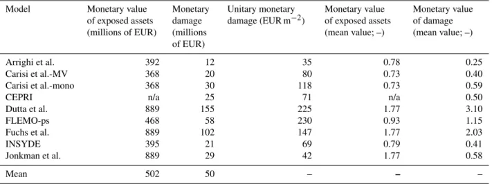
Table 3. Estimates of the monetary value of exposed assets and damage for all the buildings in the flooded area. The first column reports the total value of exposed assets (n/a: not applicable). The second and the third columns report, respectively, the total damage and the unit damage per square meter. The fourth and the fifth columns report the ratio between estimates and mean value of estimates (reported in the last row) for exposed assets and damage, respectively.
Model Monetary value
of exposed assets (millions of EUR) Monetary damage (millions of EUR) Unitary monetary damage (EUR m−2) Monetary value of exposed assets (mean value; –) Monetary value of damage (mean value; –) Arrighi et al. 392 12 35 0.78 0.25 Carisi et al.-MV 368 20 80 0.73 0.40 Carisi et al.-mono 368 30 118 0.73 0.59
CEPRI n/a 25 71 n/a 0.50
Dutta et al. 889 155 225 1.77 3.10 FLEMO-ps 468 58 230 0.93 1.15 Fuchs et al. 889 102 147 1.77 2.03 INSYDE 395 21 69 0.79 0.41 Jonkman et al. 889 29 42 1.77 0.58 Mean 502 50 – – – 3 Results
3.1 Implementation of the models to the case study in a blind mode
With the aim of understanding the impact of exposure esti-mation on damage assessment and identifying possible com-mon features in the results, Table 3 shows the total exposure and loss figures obtained by applying the nine models to all buildings within the simulated inundation area (877 in total; see Fig. 1); note that at this stage of the analysis, damage ob-servations were not considered yet for comparison purposes (see Sect. 2).
Total exposure estimates differ among the models by a maximum factor of 2.75. With respect to the mean exposure value, single estimations diverge instead by a maximum fac-tor of 1.77. These significant differences mainly result from the fact that some models calculate exposure as the monetary value of flooded floors, while others refer to the whole build-ing (see Table 2). Indeed, focusbuild-ing on the four models that consider only flooded floors (i.e. Arrighi et al., Carisi et al.-MV, Carisi et al.-mono, and INSYDE; see Table 2), total ex-posure estimates differ by a maximum factor of 1.22. Minor differences are due to the (non-)consideration of the presence of a basement as well as to the adoption of replacement or re-covery values rather than market values as parametric costs for the estimation. These results point out that a first source of variability among model outcomes lies in the approach for exposure assessment.
Total damage estimations differ among the modelling ap-proaches by a maximum factor of 12.6, which is limited to 3.1 with respect to the mean value of total damage estima-tions, suggesting that the shape of the damage functions
ex-acerbates the variability of models’ outcomes due to expo-sure estimation.
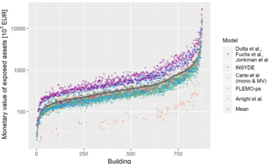
Similar conclusions can be drawn when looking at in-dividual (i.e. building by building) estimations reported in Fig. 2 (exposure values) and Fig. 3 (damage values). Individ-ual estimations of exposure differ by a mean factor of 3.5. The models of Fuchs et al., Jonkman et al., Dutta et al., and FLEMO-ps use the replacement value of the whole building as a reference for calculating the degree of loss and thus rely on sensibly higher exposure values than others. Individual damage estimates differ on average by a factor of 28, with the highest differences due to the models of Fuchs et al. and Dutta et al. (maximum expected damage) and to the model of Arrighi et al. (minimum expected damage). Such results can be partly explained by the adoption of the whole building value for exposure estimation (see also Sect. 3.2) as regards high estimations and by the zero-damage threshold for water depths lower than 0.25 m for low estimations. In detail, the weight of the zero-damage threshold on the final damage fig-ure has been calculated as a percentage ranging from 7 % to 32 %, depending on the considered model.
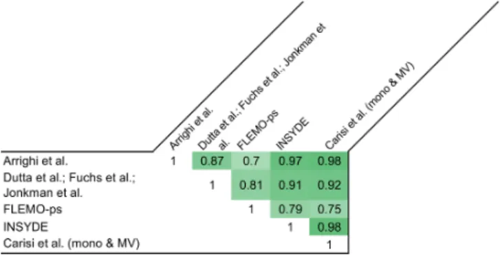
Figures 2 and 3 further highlight a common trend in ex-posure and damage values supplied by the different mod-els, also confirmed in Figs. 4 and 5, showing the Pearson’s correlation coefficients for individual (i.e. building by build-ing) exposure and damage estimates. The figures show a very high correlation of exposure estimations and a weaker, but still notable, correlation of damage estimations. This find-ing supports previous results on the importance of damage functions in determining the main differences in model out-comes. In particular, Fig. 5 shows that a higher correlation exists between absolute-damage estimates supplied by the two synthetic models INSYDE and CEPRI, among multi-variable models (INSYDE, CEPRI, Carisi et al.-MV, and
Figure 2. Individual estimates of the monetary value of the exposed assets for all the buildings in the flooded area. Data are ordered according to increasing value of mean estimate (in grey).
Figure 3. Individual estimates of the monetary damage for all the buildings in the flooded area. Data are ordered according to increasing value of mean estimate (in grey). Zero damages are due to the modelling assumptions behind the specific damage models (i.e. 0.25 m water depth threshold for damage occurrence in Arrighi et al. and 0.01 m water depth threshold in Dutta et al. and Jonkman et al. to distinguish between flooding and surface water runoff).
FLEMO-ps), and among simple models (Carisi et al.-mono, Dutta et al., Fuchs et al., Jonkman et al.), which reflects the consistency between models based on comparable concep-tual frameworks.
A comparison between correlation coefficients for absolute- and relative-damage estimations in Fig. 5 con-versely highlights the importance of exposure assessment on the final damage figures. For instance, the low correlation among absolute-damage estimates supplied by the model of Arrighi et al. with those from similar models (i.e. simple,
low-variable models like Carisi et al.-mono, Dutta et al., Fuchs et al., and Jonkman et al.) can be explained by the fact that the approach adopted by Arrighi et al. for the evalua-tion of exposure is considerably different from those adopted by the other comparable models; specifically, the model cal-culates the monetary value of damage as a function of the recovery cost, which is assumed equal to 15 % of the mar-ket value of exposed floors (see Sect. 2). Accordingly, when relative-damage estimations are considered, the values of Pearson’s correlation coefficient increase. The weight of
ex-Figure 4. Pearson’s correlation coefficient for individual exposure estimates supplied by the models with reference to all the buildings in the flooded area (the darker the colour, the stronger the correla-tion).
posure assessment is also evident when correlation among absolute-damage estimates supplied by the four simple, em-pirical models (i.e. Carisi et al.-mono, Dutta et al., Fuchs et al., and Jonkman et al.) are considered, with models of Dutta et al., Fuchs et al., and Jonkman et al. using the same exposure assessment approach (see Sect. 2) and thus be-ing more correlated among them than with the model Carisi et al.-mono; in contrast, when relative-damage estimations are considered, the correlation coefficients for the four mod-els are comparable. At last, the weight of exposure arises when correlation between absolute-damage estimates sup-plied by Carisi et al.-mono vs. INSYDE are considered. The couple consists of two conceptually different models (in par-ticular, a simple, empirical model vs. a multivariable model), but it shows high correlation. This can be explained by the adoption of very similar approaches for exposure estimation by the considered models (see Sect. 2 and Table 3); in fact, when relative-damage estimates are considered, correlation decreases.
3.2 Role of input variables in the determination of divergent models’ outcomes
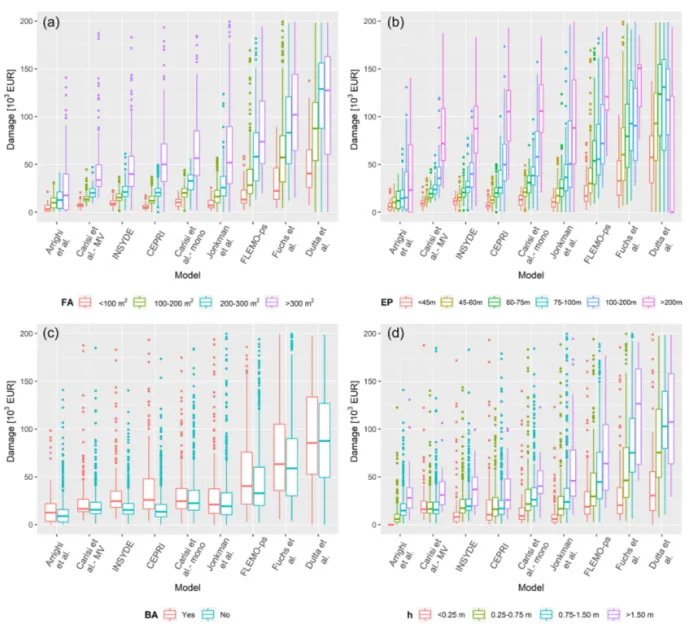
In order to explain the differences observed in the blind im-plementation, models were compared in terms of trends and variance of individual damage estimates for classes of values of input variables and by considering one variable at a time. The objectives of the analyses were to investigate whether the consideration of a specific input variable influences the out-come of a model with respect to the other ones and whether the inclusion of more explicative variables may be consid-ered as a possible source of variation as well as to identify the most influencing parameters on the final output of the models.
The input variables considered were the mean value of the water depth in the building area (h), the footprint area of the building (FA), its external perimeter (EP), the presence of a basement (BA), the building type (BT), the building structure
(BS), the finishing level of the building (FL), the number of floors (NF), and the level of maintenance (LM). The results are shown in the box plots reported in Figs. 6 and 7.
An expected increasing trend in damage as a function of the variables related to the extensive properties of the build-ings (FA and EP) can be seen, with limited data variance in the case of those models considering other explicative vari-ables than FA (e.g. EP), as INSYDE. As highlighted in the previous section, the models of Dutta et al. and Fuchs et al. show markedly different results, i.e. higher estimates than other models in all classes. This cannot be totally attributed to the fact that such models consider the whole building for calculating exposure as this is true also for the model of Jonkman et al., which supplies results that are comparable with the ones of other models. Instead, one possible reason may be found in the different origins of the models. In fact, contrarily to all other models, the model of Fuchs et al. was developed for mountainous regions, where floods are usu-ally characterized by high sediment transport and deposition, which increases the damage, other variables being equal. In the case of Dutta et al., the detection of the reason for the remarkably higher damages is more elusive given the lack of detailed information on model derivation, which makes the original model environment not known either for haz-ard or exposure variables. In addition, this model is based on survey data collected since 1954 in Japan, meaning that the data used might not be consistently representative of the current flood vulnerability (and in a European environment). The general increasing variance of the estimates with FA and EP classes can be explained by the intrinsic variability of the features characterizing larger buildings: they can be apart-ment buildings rather than semi-detached houses or big vil-las, with one or more floors; moreover, in the case of apart-ment buildings, the level of maintenance can change from flat to flat.
Figure 6 indicates the importance of BA as an influenc-ing variable in modellinfluenc-ing flood damage for the given event. This is particularly evident in the results provided by CEPRI and INSYDE, which estimate median damages ranging, re-spectively, from EUR 13 600 and 15 400 for buildings with-out a basement to EUR 26 300 and 24 500 for buildings with a basement as opposed to the performances of other models, which did not differ significantly for the two building cate-gories.
Regarding damage estimates for different water depth classes, Fig. 6 indicates an acceptable convergence among model results, especially for the shallower water depth classes, if the results of the models of Dutta et al. and Fuchs et al. are excluded (as discussed earlier). However, larger differences are apparent for the highest water depth class (h > 1.5 m). Overall, this result seems reasonable as most of the tested models were calibrated and/or validated for flood events characterized by shallow or medium inundation depths.
Figure 5. Pearson’s correlation coefficients for absolute-damage estimations (top right of the matrix; in blue) and relative-damage estimations (bottom left of the matrix; in red) supplied by the models with reference to all the buildings in the flooded area (the darker the colour, the stronger the correlation).
Figure 6. Box plots of damage estimates obtained with the tested models for different classes of footprint area – FA (a), external perimeter – EP (b), presence of basement – BA (c), and water depth – h (d). Models are organized according to increasing value of total damage estimates.
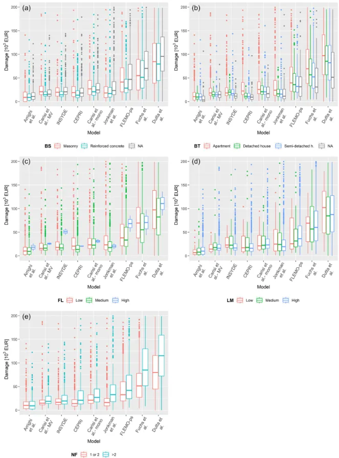
Figure 7. Box plots of damage estimates obtained with the tested models for different classes of building structure – BS (a), building type – BT (b), finishing level – FL (c), level of maintenance – LM (d), and number of floors – NF (e). Models are organized according to increasing value of total damage estimates.
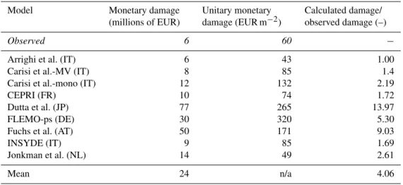
Table 4. Observed damage data vs. estimates of the total monetary damage for the subset of buildings with claims (n/a: not applicable). The second and the third columns report, respectively, the total damage and the unit value of damage per square metre. Mean value of estimates is reported in the last row. The fourth column reports the ratio between estimates and observed damage. Suffixes are used to track the original country of the models (IT: Italy; FR: France; JP: Japan; DE: Germany; AT: Austria; NL: the Netherlands).
Model Monetary damage
(millions of EUR) Unitary monetary damage (EUR m−2) Calculated damage/ observed damage (–) Observed 6 60 −
Arrighi et al. (IT) 6 43 1.00
Carisi et al.-MV (IT) 8 85 1.4
Carisi et al.-mono (IT) 12 132 2.19
CEPRI (FR) 10 74 1.72
Dutta et al. (JP) 77 265 13.97
FLEMO-ps (DE) 30 320 5.30
Fuchs et al. (AT) 50 171 9.03
INSYDE (IT) 9 85 1.69
Jonkman et al. (NL) 14 49 2.61
Mean 24 n/a 4.06
Finally, as also emerged in previous studies (Wagenaar et al., 2017; Amadio et al., 2019), Fig. 7 denotes that other variables related to building features do not significantly in-fluence model behaviour. Larger scatter is observed only for the “apartment” category, which is intrinsically characterized by larger variability, especially in terms of extensive param-eters.
3.3 Comparison between estimates and observations In order to gain knowledge on models’ reliability in the in-vestigated context, estimated losses were compared to ob-served damages derived from claims. For this purpose, a sub-set of the buildings within the simulated inundation area was considered given that claims presented by private owners were available for only 345 buildings. Table 4 summarizes the results of the sensitivity analysis by comparing the total observed damage to the total damage estimates obtained with the implementation of the nine models to the subset of build-ings. The table confirms the results presented in Sect. 3.1 (i.e. model estimations differ by a factor of around 13) and high-lights the systematic overestimation provided by the models with respect to observed damage up to a maximum differ-ence ratio of 13.97. Figure S1 in the Supplement, display-ing the ratios between estimated and observed damage at the building scale for different flood depth classes, suggests that detected differences do not depend on the hydraulic features in the inundated area but mainly on the damage models, for which the individual differences are similar across all flood depth classes. In this regard, Table 4 indicates the better per-formances of the local Italian models (marked with the “IT” suffix in the table), with Arrighi et al. showing the lowest difference. However, by looking at its features, it is possible to state that even this last model tends to overestimate
dam-Table 5. Pearson’s correlation coefficient of observed damage and estimates supplied by the models with reference to the subset of buildings with claims. The abbreviations in parentheses indicate the original countries of the models (IT: Italy; FR: France; JP: Japan; DE: Germany; AT: Austria; NL: the Netherlands).
Observed
Arrighi et al. (IT) 0.26
Carisi et al.-MV (IT) 0.10
Carisi et al.-mono (IT) 0.12
CEPRI (FR) 0.15
Dutta et al. (JP) 0.13
FLEMO-ps (DE) 0.13
Fuchs et al. (AT) 0.15
INSYDE (IT) 0.18
Jonkman et al. (NL) 0.13
age: first, because it does not consider clean-up costs (like INSYDE and CEPRI), which are instead included in the ob-servations, and second, because the lower value of the total damage with respect to other models is partly due to the ef-fect of the zero-damage threshold for water depths lower than 0.25 m (see Sect. 3.1); indeed, as highlighted in Fig. 8 (show-ing the comparison between individual observed and esti-mated damages), zero damage was expected by this model also for those buildings which experienced a significant loss. Interestingly, Table 5 finally shows that some of the im-ported models perform similarly to or better than Italian models, with particularly high performance from CEPRI.
Figure 8 generally corroborates findings of Sect. 3.1, de-picting a common trend in the models with largely different individual damage estimates. Moreover, it also emphasizes the overestimation made by the models with respect to
ob-Figure 8. Observed damage vs. individual estimates of the monetary damage for the subset of buildings with claims. Data are ordered according to increasing value of mean estimate (in black).
Table 6. Mean value of water depth (h), footprint area (FA), and external perimeters (EP) for all buildings with claims and for the outliers’ subset.
Dataset Mean value of influence variables
h(m) FA (m2) EP (m)
Outliers 0.79 264.80 78.07
All claims 0.86 265.56 77.32
servations, with the latter not showing the common trend fol-lowed by the models. This evidence is supported by the re-sults of the correlation analysis (Table 5), which reveals only marginal correlation between calculated losses and reported claims. On the contrary, the high correlation among models (see Fig. 5) raises the question of whether reported claims and damage estimation are comparable.
3.4 Analysis of damage claims
In order to explain the differences between model results and observations, a thorough analysis of claims data was carried out.
Given the general overestimation provided by the models, first we focused our attention on 44 buildings that are char-acterized by very low values of observed damage (less than EUR 1500 in 2002 currency), referred to as “outliers” here-inafter. Table 6 reports the mean value of water depth, foot-print area, and external perimeter (i.e. the variables which most influence damage according to the analysis performed in Sect. 3.2) calculated for this subset of buildings and for all the buildings with claims. Table 6 indicates that low damages cannot be explained by significant differences in these influ-encing variables given that both datasets show comparable
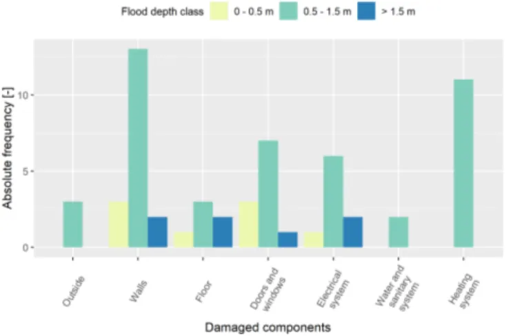
Figure 9. Absolute frequency of declared damage to the differ-ent building compondiffer-ents in the outlier dataset for differdiffer-ent water depth (h) classes.
values. Moreover, based on informal conversation with rep-resentatives of the Committee of Flooded Citizens in Lodi, it is possible to postulate that existing outliers cannot even be explained by the adoption of individual mitigation actions (like temporary flood barriers or pumps) because no official flood warning was issued, and, consequently, no lead time was available to undertake precautionary measures. Finally, from the analysis of building pictures available on Google Street View, we can state that outliers are not due to the pres-ence of steps or other elements which increase the height of the building with respect to the ground level, reducing its vul-nerability.
On the contrary, examining in detail the outlier claims, the following evidence arose:
– 27 % of outliers refer to claims with no detailed infor-mation about the type of damage, hindering the thor-ough understanding of low loss values in these cases; – 32 % of outliers can be explained by the fact that
de-clared damage regards only garages or boilers, while damage models typically assume a residential use of the building, with the presence and damage of all technical systems (i.e. heating, electrical, and water);
– 41 % of outliers refer to paltry claims, even in the case of significant water depths (around 1 m), which are mostly related to painting of walls and replacement of doors and windows.
In view of the large proportion of paltry claims, it was at-tempted to understand the causes of declared damages. For this, we calculated the frequency of damage occurrence to different building components (i.e. damage to walls, damage to floor, damage to doors and windows, and damage to sys-tems) in the different claims for three water depth classes (Fig. 9). Findings reveal an unexpected behaviour with re-spect to existing knowledge on damage mechanisms; in par-ticular the following:
– damage to floors is found to be declared mostly for wa-ter depths higher than 1.5 m, although in principle this type of damage should be poorly related to water depth; – frequency of damage to doors and windows decreases moving from the middle to the highest water depth class contrary to expectations (because of the occurrence of damage to windows with higher water depths);
– no damage to water, sanitary, and heating systems is found to be declared for water depths higher than 1.5 m, contrary to what can be expected by considering the typ-ical height of the techntyp-ical installations in Italian houses (Dottori et al., 2016).
According to our interpretation, inconsistency between ex-pected and declared damage can be attributed to the fact that what is declared by citizens does not correspond to the actual budget required to replace or reconstruct the whole physical damage suffered by the building but rather to the amount of money needed to bring the building back to a desired level of functionality according to the financial resources of the owner: for this reason, not all flooded doors, for example, are replaced nor are flooded floors always rebuilt. This would ex-plain why synthetic models overestimate observed damage as they are usually based on full replacement or reconstruction costs. Likewise, it would explain why the model by Arrighi et al. performs better than others: indeed, the recovery value adopted by this model is defined as the average difference between the market value of new buildings and that of equiv-alent older buildings requiring renovation. It is then sensible that this value reflects a balance between the two opposite ex-treme behaviours of buyers (which, in turn, depend on their
financial resources); i.e. to completely renovate the building or to bring it back to a minimum level of functioning. In our view, such behaviours can be compared with those of flooded owners.
Moreover, declared monetary damage is strongly corre-lated to the expectations that citizens have to be reimbursed. This expectation is low in Italy, when in most cases limited funding is available for the compensation of private damage, which implies strict criteria and thresholds for compensa-tion (often much lower than the effective damage). In ad-dition, all costs must be proven by the citizens by means of official invoices. For all these reasons, citizens often prefer taking advantage of the “black market” rather than declar-ing damage (Cellerino, 2004). This would also explain why empirical models (derived from claims) developed in regions with high expectations and then high values of declared dam-age (like Germany) overestimate the observed damdam-age in this case study.
From another perspective, in order to explain the scatter that is generally observed in real damage data with respect to water depth (note that the value of Pearson’s correlation co-efficient between observed damage and water depth is 0.11), we focused the attention on 13 paired buildings, whereby the term “paired” refers to buildings with the same vulnerabil-ity characteristics (i.e. building type, building structure, level of maintenance, and finishing level) as well as similar val-ues of hazard parameters (i.e. water depth and flow veloc-ity) but significant differences in the declared unit damage (EUR m−2).
The analysis revealed that
– considerable differences are attributable to declared or undeclared replacement costs of systems rather than of doors and windows (this can be explained again by what is considered to be monetary damage by citizens); – in other cases, costs related to similar damage (e.g. cost
of painting, cost of replacement of doors) differ a lot, even by a factor of 10. This discrepancy might be ex-plained by wrong assumptions concerning the finish-ing level and/or the buildfinish-ing type. More specifically, the actual conditions of buildings with high damage val-ues could have been better than what was assumed for the blind test, using cadastral data as reference (see Ta-ble 1);
– sometimes the above two factors add up, further increas-ing the differences among paired buildincreas-ings in terms of declared damage.
Scatter in claims data can then be partially explained by the influence of local parameters (like the finishing level or the building type), which are difficult to assess at the microscale without a detailed field survey; nonetheless, it seems that the influence of such parameters on damage estimation for the analysed models is very low (see Sect. 3.2) so that the latter are reliable only when applied at the mesoscale.
Overall, the analysis of claims highlighted that observed damage data need to be carefully analysed before being used for model validation since their comparability with damage estimates is not always guaranteed.
4 Discussion
Results from the previous analyses were critically analysed in order to gain general knowledge on the transferability of damage models and reliability of damage estimates as well as, in particular, to answer to the two specific research ques-tions posed in the introduction.
Concerning the performance of local vs. imported mod-els, the blind test corroborated literature results (Cammerer et al., 2013), suggesting that model transferability depends on the consistency between the context of implementation and the original calibration context as far as both hazard and exposure and vulnerability features of exposed buildings are concerned. In fact, in the blind test, models developed for the Italian territory and for riverine floods performed generally better than models derived in other countries or for differ-ent flooding features, e.g. mountain areas. Such a result was not surprising as models providing good results have proven to perform well also in other Italian validation case studies; e.g. Arrighi et al. worked well also for the 2010 flood in Veneto region (Scorzini and Frank 2017). The same applies to INSYDE and the two models by Carisi et al., which were tested in other Italian flood events (Amadio et al., 2019). In contrast, the imported model of Dutta et al. was already found to not properly work in Italian cases (Scorzini and Frank, 2017). Still, the analysis of damage claims revealed that, as far as empirical models are considered, transferabil-ity could depend also on comparabiltransferabil-ity of the compensation contexts given that observed losses on which empirical mod-els are calibrated may depend on citizens’ expectations of reimbursement.
Regarding instead the second question, the literature sug-gests that the inclusion of several influencing variables should increase the accuracy of a model (Merz et al., 2013; Schröter et al., 2014; Van Ootegem et al., 2018). Still, the blind test highlighted that such evidence can be invalidated by the lack of availability or consistency of input data be-tween the calibration and the implementation context. In-deed, the models considered in the blind test were designed to be used with the type of data usually available in the origi-nal context, which generally differ from the data available in the Lodi case study; i.e. models use different proxy variables for the same explicative parameters. For this reason, assump-tions had to be undertaken to allow the application of a model in the case study area (see Sect. 2). For example, the building categories (BTs) assumed by CEPRI (“apartment”, “single-storey building”, “multi“single-storey buildings”) are different than the Italian ones (“apartment”, “detached”, “semi-detached”) so that a correspondence has to be defined, also on the
ba-sis of the number of floors (NF); specifically apartment is defined by BT = “apartment”, “single-storey” is defined by BT = “detached” or “semi-detached” and NF = 1, “multiple storeys” is defined by BT = “detached” or “semi-detached” and NF > 1. Correspondence among building categories was defined also for the implementation of FLEMO-ps, although in this case the task was quite straightforward since the Ger-man building categories are almost coincident with the Ital-ian ones (FLEMO-ps distinguishes between “multi-family house”, “semi-detached house”, and “one-family home”). Assumptions on input variables may reduce the reliability of the original model because of an improper or inaccurate “adaptation” of the available data, thus reducing the advan-tage of using many variables. This also explains why the sim-ple models by Jonkman et al. and Carisi et al.-mono pro-vided comparable or better results than those obtained from multivariable models like FLEMO-ps or CEPRI. Also, the use of additional variables may have different impacts de-pending on whether, in the application area and differently for the original model development strategy, this information is retrieved at the building scale or known as an aggregated variable. Consultations of experts with local knowledge were needed to help in the correct interpretation and use of the available input data for the Lodi case study. Importantly, the blind test highlighted that none of the tested models (being local or imported as well as simple or multivariable) seemed appropriate to estimate flood damage at the building scale in the given context; still, models’ performance improved when aggregated damage data were taken into account. In fact, considering the 345 buildings for which a claim was known, all models’ estimates differed significantly individu-ally (Fig. 8), but some of them indicated a total damage fig-ure close to the observations (Table 4). Besides the already discussed potential biases of claim data, this duality sug-gests that model uncertainty may be balanced in aggregated results; i.e. the lump sum might be more reliable than the individual results. This raises the question of which spatial scale (that is the level of complexity) of analysis is right to get reliable results and for which objective. For example, by implementing the simpler, lump-sum model DELENAH_M (Natho and Thieken, 2018), an adaptation of the UNISDR method for national damage estimates (UNISDR, 2015) in developed countries taking Germany as a study case, the es-timate of the aggregated damage for the 345 buildings with claim data is EUR 4.3 million. This estimation is affected by an error which is comparable to or lower than errors sup-plied by the microscale models (see Table 4), although being obtained with a simple calculation and in a blind mode, i.e. using the average damage ratio for severe floods and the aver-age housing size derived from German survey data (Thieken et al., 2017) on flood losses in the housing sector (note that in this case underestimation of total damage is due to the adop-tion of a conservative housing size so that the estimaadop-tion must be intended as a minimum estimate or a lower bound). Is this assessment useful for flood risk mitigation? What is then the
advantage of using microscale models? Is there a level of spa-tial aggregation which supplies a reliable, more informative estimation than a simple lump sum at the municipality level? Answers to these questions will be the objective of further investigations by the research groups involved in the test.
5 Conclusions: lessons learnt from a modeller’s perspective
The blind test conducted in this study represented an oppor-tunity to not only deeply investigate the transferability of tested models and the reliability of their estimations, espe-cially regarding the potentialities of local and multivariable models, but also to increase authors’ awareness on strengths and limits of flood damage modelling tools. As concluding remarks, we report in the following section take-home mes-sages synthesizing lessons learnt from the blind test from a modeller’s perspective.
First, a former source of variability among models’ out-comes lies in the approach for exposure assessment, which then represents a critical, often overlooked step in flood dam-age modelling. In particular, assessing exposure coherently with the approach originally adopted in model development is key to preserve the original reliability; in this regard, the blind test showed that the different approaches applied within the models demand a clear definition and differentiation of the terms “exposure value” and “building value”. Nonethe-less, the blind test indicated a common overestimation, con-firmed also in other case studies (Zischg et al., 2018; Cam-merer et al., 2013; Thieken et al., 2008; Fuchs et al., 2019b; Arrighi et al., 2018a, b), in terms of number of buildings damaged by a flood event (i.e. the number of buildings with claims is significantly lower than those exposed to the flood). This might be attributed to the fact that not all affected build-ing owners asked for compensation or that some buildbuild-ings are not affected by the flood due to local microtopographi-cal conditions or due to the installation of protection mea-sures. However, it might also highlight problems in the cur-rent strategy adopted to identify exposure (e.g. by not con-sidering building elevation).
A second critical issue in flood damage modelling is the transfer of models in space and time, with difficulties in pre-dicting the expected performance of a given model when ap-plied in a different context (e.g. Jongman et al., 2012; Cam-merer et al., 2013; Wagenaar et al., 2018). Accordingly, flood damage modellers should always be cautious when apply-ing a flood damage model to a new context. Their general trust in the model performance in the new study area must be in the first instance limited; however, model validation (ideally, over multiple datasets) can significantly increase the trust level.
But validation of damage models invariably relies on ob-served damage data, either from insurance claims, govern-mental reimbursement claims, or direct surveys, all of which
are generally intended as “reality”. Indeed, it is often the case that empirical data are used in validation analyses without any possible preliminary evaluation on their quality and sig-nificance simply because no ancillary information is avail-able, as for instance for insurance data (André et al., 2013; Spekkers et al., 2013; Zhou et al., 2013; Wing et al., 2020). In this context, the blind test highlighted that “reality” de-picted by observations is not univocal so that observed data must be carefully investigated before their comparison with model outcomes as they may be addressing different types of damage or damage to different components, or they may be incomplete. Based on this consideration, flood damage modellers must always be cautious when drawing conclu-sions from validation analyses: if a model does not fit well to some empirical data, this does not necessarily reflect the inability of the model in general terms, but attention has to be drawn to input data quality and vice versa. This also points out the importance of collecting not only flood damage data but also ancillary information on flood hazard and vulnerabil-ity of affected assets in the ex-post flood phase (Merz et al., 2004; Thieken et al., 2005, 2016; Ballio et al., 2018; Moli-nari et al., 2017, 2019). Moreover, consultations of experts with local knowledge can help in the correct interpretation and use of observed damage data.
In absence of data (or appropriate data) for validation, the application of several models might be useful to quantify mean and variance and provide a range of uncertainty of the estimations (Figueiredo et al., 2018); a good agreement of model results, in particular with the models developed for contexts similar to the one under investigation, can signifi-cantly increase the trust level in model performance. In this regard, the blind test stressed that damage models have to be compared in their original form, meaning that, for instance, relative-damage models relying on the total building value cannot be directly compared to the ones relying on only the first floor.
As a general recommendation, to select a damage model for an application in a different country, it is important to verify the comparability between the original and the in-vestigated physical (in terms of hazard and building fea-tures) and compensation context as well as the availability and coherence of the input data. Moreover, when transfer-ring a model (in space or time), proxies of input variables are frequently needed, and the modeller must be prudent in this step. A good understanding of both the data used dur-ing the model development and the data gathered for the new application is crucial as the attribution of uncertainty be-comes elusive afterwards if this step is neglected. The blind test highlighted that the real effort of transferring the mod-els to the given implementation context was related to find-ing the “right” required data, while the costs of implement-ing assumptions about exposure and calculatimplement-ing the dam-age value were negligible. To support transferability, there is then a need to precisely describe how the models were de-veloped, which variables were included, and for which