21 cm cosmology with optimized instrumentation and algorithms

21 cm Cosmology

with Optimized Instrumentation and Algorithms

by

Haoxuan Zheng

B.S., University of Richmond (2011)

Submitted to the Department of Physics

in partial fulfillment of the requirements for the degree of

Doctor of Philosophy

at the

MASSACHUSETTS INSTITUTE OF TECHNOLOGY

June 2016

@

Massachusetts Institute of Technology 2016. All rights reserved.

Auho.Signature

redacted

A uthor.

...

Signature redacted

C ertified by . ...

April 29, 2016

Max Tegmark

Professor of Physics

Thesis Supervisor

Accepted by ...

Signature redacted...

Nergis Mavalvala

JUN 0

9

2016

LIBRARIES

Professor of Physics

Associate Department Head for Education

21 cm Cosmology

with Optimized Instrumentation and Algorithms

by

Haoxuan Zheng

Submitted to the Department of Physics on April 29, 2016, in partial fulfillment of the

requirements for the degree of Doctor of Philosophy

Abstract

Precision cosmology has made tremendous progress in the past two decades thanks to a large amount of high quality data from the Cosmic Microwave Background (CMB), galaxy surveys and other cosmological probes. However, most of our universe's vol-ume, corresponding to the period between the CMB and when the first stars formed, remains unexplored. Since there were no luminous objects during that period, it is called the cosmic "dark ages". 21 cm cosmology is the study of the high redshift uni-verse using the hyperfine transition of neutral hydrogen, and it has the potential to probe that unchartered volume of our universe and the ensuing cosmic dawn, placing unprecedented constraints on our cosmic history as well as on fundamental physics.

My Ph.D. thesis work tackles the most pressing observational challenges we face in the field of 21 cm cosmology: precision calibration and foreground characterization. I lead the design, deployment and data analysis of the MIT Epoch of Reionization

(MITEoR) radio telescope, an interferometric array of 64-dual polarization antennas whose goal was to test technology and algorithms for incorporation into the Hydrogen Epoch of Reionization Array (HERA). In four papers, I develop, test and improve many algorithms in low frequency radio interferometry that are optimized for 21 cm cosmology. These include a set of calibration algorithms forming redundant calibra-tion pipeline which I created and demonstrated to be the most precise and robust calibration method currently available. By applying this redundant calibration to high quality data collected by the Precision Array for Probing the Epoch of Reion-ization (PAPER), we have produced the tightest upper bound of the redshifted 21 cm signals to date. I have also created new imaging algorithms specifically tailored to the latest generation of radio interferometers, allowing them to make Galactic fore-ground maps that are not accessible through traditional radio interferometry. Lastly, I have improved on the algorithm that synthesizes foreground maps into the Global Sky Model (GSM), and used it to create an improved model of diffuse sky emission from 10 MHz through 5 THz.

Thesis Supervisor: Max Tegmark Title: Professor of Physics

Many are stubborn in pursuit of the path they have chosen, few in pursuit of the goal.

Contents

Acknowledgments 1 Introduction

1.1 Precision Cosmology . . . . 1.1.1 The Far End: the Cosmic Microwave Background 1.1.2 In the Neighborhood: the Galaxy Surveys . . . . 1.1.3 Is There Anything in between? . . . . 1.2 Probing the Red-shifted Neutral Hydrogen Gas and the 21 cm Cosmology . . . . 1.2.1 Temperature Evolution of the Neutral Hydrogen 1.2.2 The 21 cm Power Spectrum . . . . 1.2.3 The Potential of 21 cm Cosmology . . . . 1.3 Low-frequency Radio Interferometry . . . . 1.3.1 Basic Instrumentation . . . . 1.3.2 Calibration . . . . 1.3.3 Im aging . . . . 1.3.4 Challenges in 21 cm Cosmology Instruments 1.4 Thesis Outline . . . . 17 19 19 20 20 21 Potential Gas of 25 25 27 28 28 30 31 . . . . . 32 . . . . . 34 . . . . . 35

Part I

Building MITEoR and OMNICAL

37

2 MITEoR: A Scalable Interferometer for Precision 21 cm Cosmology 39 2.1 Introduction . . . . 39 2.2 The MITEoR Experiment . . . . 43

2.2.1 The Ana 2.2.1.1 2.2.1.2 2.2.1.3 2.2.1.4 2.2.2 The Digi 2.2.3 MITEoR 2.3 Calibration Rest 2.3.1 Relative 2.3.1.1 2.3.1.2 2.3.1.3 2.3.1.4 2.3.1.5 log System . . . . Antennas . . . . Swappers (Phase Switches) . . . . Line-Driver . . . . Receiver . . . . tal System . . . . . Deployment and Data Collection . . . . lts . . . . Calibration . . . . Overview . . . . Rough Calibration . . . . Log Calibration and Linear Calibration . . .

x

Quality

45 46 46 48 49 50 53 54 55 55 57 58 61 64 2.3.2 Absolute Calibration . . . . 68

2.3.2.1 Breaking Degeneracies in Redundant Calibration 2.3.2.2 Beam Measurement Using ORBCOMM Satellites 2.3.2.3 Calibrating Array Orientation Using ORBCOMM

Satellites and the Sun . . . . 2.3.3 System atics . . . . 2.4 Summary and Outlook . . . . 2.A Appendix: Phase Degeneracy in Redundant Calibration . . . . 2.B Appendix: A Hierarchical Redundant Calibration Scheme with O(N) Scalin g . . . . 2.C Appendix: Fast Algorithm to Simulate Visibilities Using Global Sky M od el . . . . 2.C.1 Spherical Harmonic Transform of the GSM . . . . 2.C.2 Spherical Harmonic Transform of the Beam and Phase Factors 2.C.3 Computing Visibilities . . . . 69 70 76 79 82 83 87 90 91 92 93 8

Part II Latest Epoch of Reionization Science Results

3 PAPER-64 Constraints on Reionization: the 21 cm Power

Spec-trum at z = 8.4 97 3.1 Introduction . . . . 3.2 Observations ... 3.3 Calibration ... 3.3.1 Relative Calibration . . . 3.3.2 Absolute Calibration . . . 3.3.3 Wideband Delay Filtering 3.3.4 Binning in LST . . . . 3.3.5 Fringe-rate Filtering . . . 3.4 Instrumental Performance . . . . 3.4.1 Instrument Stability . . . 3.4.2 System Temperature . . .

3.5 Power Spectrum Analysis . . . .

3.5.1 Review of OQEs . . . . . 3.5.2 Application of OQE . . .

3.5.3 Covariance Matrix and Signal Loss 3.5.4 Bootstrapped Averaging and Errors 3.6 R esults . . . .

3.6.1 Power Spectrum Constraints . . . .

3.6.2 Spin Temperature Constraints . . . 3.7 Discussion . . . . 3.8 Conclusions . . . .

Part III Novel Imaging and The New Global Sky Model

152

4 Low Frequency Mapmaking with Compact Interferometers: A

MI-TEoR Northern Sky Map from 128 MHz to 175 MHz 153

95 97 100 103 105 109 113 114 116 118 118 121 123 123 126 133 137 140 140 145 148 149

4.1 Introduction . . . . 153

4.2 Wide Field Interferometric Imaging . . . . 157

4.2.1 Fram ework . . . . 157

4.2.2 Constructing the A-Matrix . . . . 159

4.2.3 Regularization and Point Spread Functions . . . . 160

4.2.4 Wiener Filtering and Incorporating Prior Knowledge . . . . . 162

4.2.5 Further Generalization . . . . 164

4.3 Sim ulations . . . . 165

4.3.1 MITEoR Simulation . . . . 165

4.3.2 MWA Simulation . . . . 166

4.3.3 Simulation Discussion ... . . . . 168

4.4 New Sky Map . . . . 170

4.4.1 MITEoR Instrument and Data Reduction . . . . 170

4.4.1.1 Absolute Amplitude Calibration . . . . 171

4.4.1.2 Absolute Phase Calibration . . . . 173

4.4.1.3 Cross-talk Removal . . . . 174

4.4.2 Northern Sky Map Combining Multiple MITEoR Frequencies 174 4.4.3 Error Analysis . . . . 176

4.4.4 Spectral Index Results . . . . 177

4.4.4.1 Spectral Indices from 128 MHz to 175 MHz . . . . 177

4.4.4.2 Spectral Indices from 85 MHz to 408 MHz . . . . 179

4.5 Summary and Outlook . . . . 180

4.A Appendix: Improvements to Redundant Calibration . . . 182

4.B Appendix: Dynamic Pixelization . . . 185

5 An Improved Model of Diffuse Galactic Radio Emission from 10 MHz to 5 THz 187 5.1 Introduction . . . 187

5.2 Iterative Algorithm for Building a Global Sky Model . . . 190

5.2.1 Fram ework . . . 190 10

5.2.2 PCA Algorithm ... ... 191

5.2.3 Iterative Algorithm . . . . 192

5.2.4 Incorporating More General Data Formats . . . . 193

5.3 Sky Survey Data Sets . . . . 194

5.4 Results: the Improved Global Sky Model . . . . 195

5.4.1 Orthogonal Components Result . . . . 195

5.4.2 Error Analysis . . . . ... . . . . 198

5.4.3 Blind Component Separation . . . . 200

5.4.4 Fitting the Blind Components . . . . 202

5.4.5 High Resolution GSM . . . . 203

5.4.6 Further Discussion . . . ... . . . . 205

5.5 Summary and Outlook . . . . 206

6 Conclusion 209

List of Figures

1-1 The evolution of CMB anisotropy measurements. . . . . 1-2 The Planck power spectrum . . . . 1-3 SDSS Legacy Survey. . . . . 1-4 Our Hubble volume. . . . . 1-5 A schematic picture of the Cosmic Dawn .. . . . . 1-6 Simulations of the global 21 cm signal. . . . . 1-7 Simulated hydrogen cube undergoing reionization and its evolving power

specrtrum . . . . 1-8 V LA im ages. . . . . 2-1 System schematic of an FFT telescope. . . . . 2-2 MITEoR analog system design. . . . . 2-3 MITEoR swapper design .. . . . .

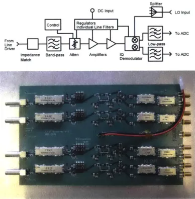
Laboratory measurements of cross-talk with and without the Schematic and photograph of the line drivers. . . . . Schematic and photograph of the receiver boards. . . . . Photograph of the MITEoR computer rack. . . . . Photograph of the 2013 MITEoR deployment. . . . . Redundant calibration during an ORBCOMM satellite pass. x2 as a function of time and frequency waterfall plot...

x2 _{histograms of redundantly calibrated data. . . . .}

Illustration of Weiner filtering calibration solutions. . . . . . Waterfall plot of a full day's data compared to a simulation. ORBCOMM trajectories through the primary beam...

swapper. 48 . . . . . 49 . . . . . 50 . . . . . 51 . . . . . 54 . . . . . 56 . . . . . 61 . . . . . 63 . . . . . 67 . . . . . 71 . . . . . 74 12 20 21 22 23 24 27 29 30 44 46 47 2-4 2-5 2-6 2-7 2-8 2-9 2-10 2-11 2-12 2-13 2-14

2-15 Measured primary beam using ORBCOMM satellite passes. ... 75

2-16 Calibration of array orientation using ORBCOMM. . . . . 77

2-17 Investigation of signal-dependent systematic error. . . . . 81

2-18 Illustration of phase degeneracies with short baselines. . . . . 86

2-19 Illustration of phase degeneracies without short baselines. . . . . 87

2-20 Schematic of heirarchical calibration method . . . . 88

3-1 Antenna position within the PAPER-64 array. . . . . 101

3-2 The Global Sky Model illustrating foregrounds to the 21cm cosmolog-ical signal. . . . . 102

3-3 The stages of power-spectrum analysis. . . . . 104

3-4 PAPER visibilities plotted in the complex plane before and after the application of the improved redundancy-based calibration with OM-N IC A L . . . . 107

3-5 Log of

X

3-6 PAPER-64 image of a field including Pictor A and Fornax A . . . 111

3-7 Measured spectrum of Pictor A in Stokes I relative to its catalog value. 112 3-8 Visibilities measured by a fiducial baseline in the PAPER-64 array. . 115 3-9 The optimal fringe-rate filter and the degraded fringe-rate filter. . . . 119

3-10 Histogram of the real component of all calibrated visibilities measured over 135 days. . . . . 119

3-11 Power spectrum of 135 days of time-series data contributing to a single L ST bin. . . . . 120

3-12 System temperature inferred from the variance of samples falling in an L ST bin. . . . . 122

3-13 Visibilities before and after inverse covariance weighting. . . . . 129

3-14 Eigenvalue spectrum of covariance matrices (left) empirically estimated from visibilities. . . . . 130

3-15 The window function matrix W. . . . . 134

3-16 Recovered power spectrum signal as a function of injected signal

am-plitude. . . . . 136

3-17 Absolute value of the cumulative mean and median as a function of number of modes of the power spectrum band power. . . . . 138

3-18 Measured power spectrum at z = 8.4 resulting from a 135 day obser-vation with PAPER-64 . . . . 141

3-19 Diagnostic power spectra. . . . . 142

3-20 Posterior distribution of power spectrum amplitude for a flat A2 _(k) power spectrum over 0.15 < k < 0.5h Mpc-1 . . . . 144

3-21 Constraints on the 21cm spin temperature at z = 8.4. . . . . 145

4-1 Simulated results for MITEoR, the MWAcore, and the two combined. 167 4-2 Output maps recovered in simulation and their error bars using differ-ent regularization matrices. . . . . 168

4-3 MITEoR's observing schedule and a small subset of the MITEoR data product. ... ... 171

4-4 MITEoR map result. . . . . 175

4-5 Overall spectral index fit and beam-averaged spectral index over LST. 178 4-6 Spectral index maps. ... ... 181

4-7 Dynamic pixelization scheme. . . . . 186

5-1 29 sky maps used in this work from 10 MHz to 5 THz. . . . . 194

5-2 The overall amplitudes of the 29 sky maps. . . . . 195

5-3 The 6 orthogonal components and their spectra. . . . . 197

5-4 Three different RMS error percentage estimations for our GSM. . . . 198

5-5 The 6 recombined components that roughly correspond to various physical mechanisms. . . . 201

5-6 High resolution version of the six component maps. . . . 205

List of Tables

2.1 M ITEoR specifications.. . . . . 53

2.2 Effects of Wiener filtering calibration solutions. . . . . 68

3.1 Signal loss versus analysis stage. . . . 137

4.1 A 4 by 4 antenna array on a regular grid. . . . . 184

5.1 List of sky maps we use in our multi-frequency modeling. . . . . 196

5.2 List of model parameters for our blind components compared to exist-ing literature values. . . . . 204

Acknowledgments

I am truly grateful to my advisor, Prof. Max Tegmark, without whom I could not have enjoyed such an exciting and fulfilling five years as a graduate student. The many lessons I learned from him have not only been invaluable assets to my Ph.D. career, but will remain so to all my years ahead. I would also like to thank my thesis committee members, Prof. Jacqueline Hewitt and Prof. Paolo Zuccon, for their time and guidance that helped shape this thesis.

I would like to thank my lovely wife, Sherry, for her unending love and support. She has made many sacrifices for me so that I can pursue my passion and curiosity. Having her in my life is the best thing that has ever happened to me.

I would like to thank my mom and dad: nature or nurture, they are the ones who helped me become who I am today, and I'm truly grateful for having such wonderful parents.

Last but not least, I would like to thank my academic brothers, Adrian Liu and Josh Dillon, who have spent countless hours helping me with my projects and papers, and from whom much of this thesis inherit from. I also want to thank my friend Abraham Neben, with whom, I have shared so many enjoyable conversations in and outside physics.

Chapter 1

Introduction

1.1

Precision Cosmology

Precision cosmology has made tremendous progress in the past two decades, thanks to a large amount of high quality data from the Cosmic Microwave Background (CMB) as well as the study of nearby stars and galaxies. As my advisor Max likes to say, when he was a graduate student 25 years ago, people were arguing over whether our universe is 10 billion years old or 20 billion years old, whereas nowadays, people debate over whether it is 13.7 or 13.8 billion years old. This drastic improvement in our knowledge of our universe's age is only the tip of the iceberg that is the triumph of precision cosmology. As another example, we now know that our universe consists of only about 5% ordinary matter that constitutes everything around us here on Earth, and the other 95% is split between about 26% dark matter and 69% dark energy [134]. The physical natures of dark matter and dark energy remain mysteries to us, but perhaps another two decades of precision cosmology could unveil their secrets. In the next two sections, I will briefly review two of the most important topics in precision cosmology: the Cosmic Microwave Background (CMB) and the 3D mapping of galaxies through the Sloan Digital Sky Survey.

Figure 1-1: The evolution of CMB anisotropy measurements made by the last, three generations of CMB experiments. Image credits: the COBE, WMAP, and Planck

Collaborations, respectively.

1.1.1

The Far End: the Cosmic Microwave Background

The CMB is a blackbody radiation emitted by cooling plasma in the early universe when it cooled to about 3,000 K, less than half a million years after our Big Bang. As the CMB radiation traveled to us, it cooled down by a. factor of about 1100, so it ap-pears to us as 2.725 K blackbody radiation. Because the 2.725 K blackbody spectrum peaks in the nmicrowave band, it, is called the Cosmic Microwave Background. This radiation was discovered back in the 1960s. Most of the recent progress in cosmology has come from studying very slight variations in CMB temlperature throughout the sky, typically no more than 0.1 mK. Fig. 1-1 clearly shows the improvement, in quality, specifically angular resolution and sensitivity, of the last three generations of CMB experiments, which are all microwave detectors nounted on satellites. People study the CMB anisotropy by investigating the statistical property of the anisotropies, cap-tured by the CMB power spectrum, as shown in Fig. 1-2. The strength of the power spectrum represents the amount. of fluctuation concentrated at various angular scales, and the amplitudes and locations of the peaks in the power spectrum are determined

by what happened both before the CMB was emitted, as well as when it. was on its

way to us. Thus, careful study of the power spectrum can and has revealed a great, deal about the history of our universe.

1.1.2

In the Neighborhood: the Galaxy Surveys

Observing stars in our Galaxy and other distant galaxies have been the study of astronoiny for centuries. Edwin Hubble's observation in 1929 that the majority of distant galaxies are moving away from us is perhaps one of the most impactful

dis-20

ONEEMIL-Multipole moment, f 2 10 50 500 1000 1500 2000 2500 C 6000 5000 U, C 0 4000 2000 1000 I- 0 90 18 ' 0.2' 0.1' 0.07 Angular scale

Figure 1-2: The CMB power spectrum measured by the Planck satellite. Our current cosmological model (green curve) can fit it, very well with just six parameters. Image credit: Uhc Planck Collaborations.

coveries in the history of cosmology. The constant development of more and more advanced telescopes and spectroscopes has allowed us to observe more galaxies that are farther away. One of the most ambitious efforts in systematically studying galax-ies is the Sloan Digital Sky Survey [190] (SDSS). Using the 2.5 im telescope at Apache Point Observatory, the SDSS created the largest volume three-dimensional map of galaxies to date (see Fig. 1-3).

1.1.3

Is There Anything in between?

The 13.8 billion years old CMB is at, the far end of our universe accessible to us through light. This is because before the time when CMB was emitted, the hot plasma that filled the universe did not, allow light to travel freely. On the other hand. most of the galaxies surveyed by SDSS are less than 2 billion years old', which is

very close to us compared to the CMB. Thus, one must be tempted to ask: is there anything we can observe in between the CMB and the oldest galaxies? If observations of the farthest, slice (CMB) and the nearby volume (SDSS) have propelled the last,

'SDSS has been carrying out larger and larger surveys, and other instruments have observed

galaxies more than 10 billion years old. However, volume in cosmology is not proportional to the

age cubed, so the gap between the CI\4B and the oldest galaxy is much larger thaii their age gaps suggest. See Fig. 1-4.

-Figure 1-3: The 3D galaxy map made by the SDSS Legacy Survey. Each point in this "cosmic web" is a galaxy, and the farthest galaxies are about 2 billion years old.

Image credit: the Sloan Digital Sky Survey.

two decades of cosmological discoveries, observing the volume in between certainly has the potential to revolutionize cosmology again.

As shown in Fig. 1-4, the missing gap actually makes up more than 80% of our universe's comoving volume. This gap period has been called the cosmic dark ages, because there was very little light being generated then, compared to the later times when our universe is populated by shiny stars and galaxies. Fortunately, the universe was not, a complete void, but was filled by neutral hydrogen gas, which later gravitated to form the stars and galaxies. What is more, the neutral hydrogen gas did emit radiation that we can observe today. Unlike the CMB which obeys a continuous spectrum characteristic of the blackbody radiation, the neutral hydrogen atoms have a hyperfine transition that. emit light, at a very specific wavelength: 21 cm. As the 21 cm radio waves traveled towards us, their wavelength got stretched due to the universe's expansion, and the earlier they were emitted, the more they were stretched. This, combined with the fact that the neutral hydrogen is optically thin, allows us to determine the age of any emission from neutral hydrogen by simply looking at how much longer its wavelength is compared to 21 cm, so in principle we can make a 3D map of the entire gap shown in Fig. 1-4.

\Ve Cosmic Microw

=1100

Figure 1-4: The CMB anisotropy maps and the galaxy surveys only probe a small fraction of the volume of the observable universe. 21 cm cosmology, the probe that this thesis focuses on developing, may one day make the entire pink region accessible to direct observation. Image credits: Josh Dillon and Tegmark and Zaldarriaga [166.

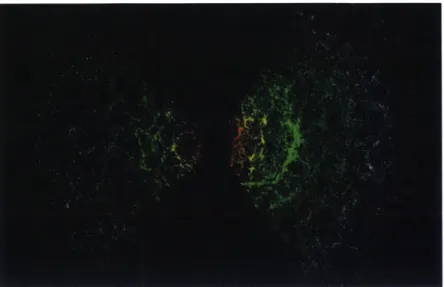
Figure 1-5: The Epoch of Reionization is a period in the early history of the universe between the cosmic microwave background (on the left) and modern stars and galaxies (on the right). During this time, the first stars and galaxies form and ionize the neutral hydrogen gas around them, which creates merging bubbles of ionized hydrogen. Image

credit: Abraham Loeb and Scientific American.

Being able to map the neutral hydrogen throughout the history of our universe can shed much light. on both cosmology and astrophysics. The neutral hydrogen gas underwent a lot of changes during the dark ages, especially towards the end when the first stars and galaxies just started forning (which we call the "cosmic dawni"). The young stars and galaxies emitted strong radiation that ionized the neutral hydrogen around them (in a process called reionization), and the hydrogen gas stopped emitting 21 cm radiation once ionized. Thus, if we can make a 3D hydrogen map, we can see that more and more empty "bubbles" appeared and merged during the cosmic dawn, as shown in Fig. 1-5. Currently we have a rough idea of how it might, have happened, but, we don't, even know exactly when this "bubble period" was, how long it lasted, or any further details. Thus, direct measurements of this transition period will teach us about both the structure of our universe, as well as the formation of the first stars and galaxies.

1.2

Probing the Red-shifted Neutral Hydrogen Gas

and the Potential of 21 cm Cosmology

In this section I briefly describe the more technical aspects of 21 cm cosmology. For a much more detailed review, see the introduction of Josh Dillon's thesis [35] and reviews in the literature [54, 144],

1.2.1

Temperature Evolution of the Neutral Hydrogen Gas

The aforementioned 21 cm radiation has been observed and used to trace neutral hydrogen in our Galaxy since its first detection in 1951 by Ewen and Purcell [44]. However, it is different to probe the neutral hydrogen before and during the epoch of reionization (EoR) with red-shifted 21 cm signals. For periods before and during the EoR, the hydrogen gas is observed in the form of either emission or absorption relative to the CMB. What we directly measure is I,, the specific intensity of emission at the frequency v. Since the red-shifted 21 cm signals have frequencies on the order of 10' Hz, much lower than the peak of the CMB at around 10" Hz, we can use the Rayleigh-Jeans limit of the blackbody spectrum to represent observed specific intensities as brightness temperatures Tb, where

2kBTbl2

Iv = 2 (1.1)

The observed brightness temperature is a combination of the CMB temperature Ty-and the spin temperature of the hydrogen gas Ts, which is defined in terms of the Boltzmann factor for the spin-singlet and spin-triplet hyperfine levels of the ground state of hydrogen,

ntriplet = 3ehv0/k S. (12

nsinglet

Following Furlanetto et al. [54], the equation of radiative transfer through a cloud of hydrogen backlit by the CMB is

where -r, is the optical depth of the cloud due to the 21 cm transition.

Since the neutral hydrogen gas is considered optically thin (T, < 1) [54], contrast in the 21 cm signal observed today relative to the CMB is then given by

Tb (z) _ 6Ta bs(z) _b1 = _{+ z} -T,(z _TY( = 0) (Ts(z) - T,(z)) (1 - e-TVo) I + z Ts(z) - Ty(z) I + z 7V 14

where T,0 is the integrated optical depth over frequency. Finally, we skip some

tech-nical calculations shown in Furlanetto et al. [54] and Pritchard and Loeb [144], and arrive at the final equation

,b, (Z - 7-(z 1+ (1 + z)H(z)

6Ta

TS(z) 10

L

'

(1.5) where XHI is the neutral fraction of the hydrogen gas (with 1 meaning fully neutral), 6_b

is the baryon over-density, H(z) is the Hubble parameter, and 0v1o

/&rl

of the proper velocity along the line of sight.

Equation 1.5 shows that the observed brightness temperature depends on the relative amplitude of the spin temperature and the CMB temperature. As discussed in Furlanetto et al. [54], Pritchard and Loeb [144], the spin temperature is driven by three major processes: interaction with CMB photons, collisions between neutral hydrogen atoms and other particles, and absorption and remission of Lyman-alpha photons known as the Wouthuysen-Field effect [187, 48]. In equilibrium, the spin temperature is given by

_, T-1 + XCTy + -1

T T 1 + xT + x ~T (1.6)

where xc and x, are the collisional and Lyman-alpha coupling coefficients, TK is

the kinetic temperature related to particle collisions, and T. is the Lyman-alpha temperature related to the Wouthuysen-Field effect. Since many of these

U EW

Time after 10 million 100 million 250 million 500 million 1 billion

Big Bang 60

[Years]

Redshift=160 80 40 20 15 14 13 12 11 10 9 8 7

50

First galaxies form

-E 0 -- - --- ^----~ - - -~ -- - - - T Reoiainbgn -i on izat i-6n- bei n-s~ - ~ eionization enda

---i -t-on -nd

S -50

Dark Ages -100

Heating begins Cosmic time

-150

0 20 40 60 80 100 120 140 160 180 200

Frequency [MHz]

Figure 1-6: Top: simulated evolution of the brightness temperature, driven by the formation of the first stars and galaxies. Bottom: the sky-averaged global 21 cm signal calculated from the simulated result in the top panel. Reproduced from Pritchard and Loeb [J441.

ties are inhomogeneous and change across cosmological time, so does the brightness temperature we observe. The top panel of Fig. 1-6 shows simulated evolution of the brightness temperature. However, the precise physical processes that drive this evolu-tion are poorly understood, and precise measurements on the evoluevolu-tion of brightness temperature during EoR will shed light on these topics [54, 144].

1.2.2 The 21 cm Power Spectrum

While making high quality 3D maps of the brightness temperature will be

possi-ble in the future, current efforts are focusing on reduced data, products due to low

signal-to-noise ratio in today's instruments. The simplest data product that. probes the evolution of the brightness temperature is the global 21 cm signal, which is the brightness temperature averaged over the whole sky, as shown in the bottom panel of Fig. 1-6. Another useful reduced data Iproduct is the power spectrum of the bright-ness temperature. This power spectrum P(k) reflects the amount of correlation on various length scales k in the 21 cm brightness temperature, and it is defined by

where 6Tb(k) is the spatial Fourier transform of 6Tb(r). If we approximate the spatial distribution of 6Tb(r) as isotropic, we turn P(k) into P(k), and obtain the dimen-sionless power spectrum

k3

1(k) = 2 2 P(k). (1.8)

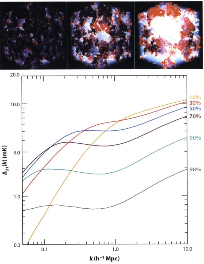
As reionization progresses, both the number and the size of ionized bubbles in-crease, so we expect to see more and more power at lower k, and less and less power overall. Fig. 1-7 shows simulated evolution of the power spectrum from 10% ionized to 98% ionized. Measuring the evolution of the 21 cm power spectrum is the focus of many current instruments, including the ones presented in this thesis.

1.2.3

The Potential of 21 cm Cosmology

Precise measurements of the red-shifted 21 cm signals will not only shed light on the astrophysical processes driving reionization, but also teach us a lot more about our universe. Pober et al. [139] has shown that a suitably designed instrument with a tenth of a square kilometer of collecting area will allow tight constraints on the timing and duration of reionization and the astrophysical processes that drove it. As shown by Mao et al. [93], a future radio array with a square kilometer of collecting area, maximal sky coverage, and good foreground maps could improve the sensitivity to cosmological parameters, such as spatial curvature and neutrino masses, by up to two orders of magnitude. It also has the potential to shed new light on the early universe by measuring the running of the spectral index related to the theory of inflation. In the shorter term, Liu et al. [88] has shown that with the instruments currently under construction, it is possible to constrain some of the cosmological parameters much better than the CMB experiments can.

1.3

Low-frequency Radio Interferometry

The first generation of instruments designed to measure the 21 cm power spectrum are all radio interferometers [75, 172, 125, 188, 115, 60], and they have inherited

20.0 _{11111 I I 111111 I I I 11111} 10.0 30% - 50% 70%

E3.0

k

(h

_Mpc)

Figure 1-7: Simulated evolution of a hydrogen cube undergoing reionization (top), and simulated evolution of the power spectrum (bottom). As the number and the size of ionized bubbles increase, there is more and more power at lower k:, and less and less power overall. Image credit: Marcelo Alvarez, Ralf Kaehler, and Tom Abel

Figure 1-8: The Very Large Array (VLA, on the left) is a radio interferometer that consists of 27 radio antennas located at the NRAO site in Socorro, New Mexico. Each antenna in the array measures 25 meters in diameter and weighs about 230 tons. The first, direct observation of an Einstein ring (middle figure) was made using the VLA

by a team led by Prof. Jacqueline Hewitt, whom I have the honor to have on my

thesis committee. This 1986 observation of the quasar 3C175 (on the right) has a

0.35 arcsecond resolution. Inage credit: National Radio Astronomy Observatory and the Very Large Array.

many ideas from traditional radio interferometry developed in the past century. One example of an exquisite radio interferometer and its amazing achievements are shown in Fig. 1-8. Before we discuss more about new challenges in 21 cm instrumentation and how I optimized algorithms and instrumentations for detecting 21 cm signals, I would like to give a, brief introduction to fundamental radio interferometry in this section, which will help us understand the need for new algorithms in 21 cm interferometry.

1.3.1

Basic Instrumentation

Very roughly speaking, the signal chain in radio interferometers can be divided into four stages: detection, amnplification, digitization, and cross-correlation. Radio fre-quency emissions are usually detected using antennas, which themselves are typically similar in size to the wavelength they are designed to detect, ranging from millime-ters to memillime-ters. The large dishes, such as those in Fig. 1-8, are reflectors designed to increase sensitivity by reflecting niuch more radiation onto the antennas, which are located at the focal points of the dishes. The signals picked up by the antennas are first amplified by low noise amplifiers, before they are digitized by analog-to-digital converters (ADCs). At this stage, the output of an ADC connected to the ith antenna

can be described using incident plane wave, summed over all directions in the sky:

Ei(t) = _{s(k, t)b(i)ei(k-ri-wt)dQ, (1.9)}

where k is the wave vector of radiation coming from sky direction k, s(k, t) is the strength of signal coming from that direction at the moment t in time, b(k) is the antenna's sensitivity in that direction decided by the shape of the antenna and its reflector, and ri is the antenna's position on the ground. For simplicity I have omitted the noise term here.

Since the radio frequency is in the MHz-GHz range, it is not convenient to record millions or billions of samples of Ei(t) for every antenna onto a hard drive directly. However, since the signals oscillate rapidly, any averaging over time would severely reduce their amplitude. To solve this problem, people cross-correlate signals to form so-called visibilities from pairs of antennas:

vig(t) = (E'(t)Ej(t))

J

where * means complex conjugate, S =sl2, and B = Ib|2. The eik(rjri) term is the interference pattern between the two antennas; thus the name interferometer. In this form, the fast varying wt-terms are canceled, and the only remaining t-dependence is in S(k, t), which varies on the time scale of Earth's rotation. Thus, we can safely integrate the visibilities over tens of milliseconds. Even longer integration is possible, depending on the angular resolution of the instrument. For high resolution instru-ments like the VLA, integration over timescales of minutes can be done through techniques such as delay tracking, which compensates for the movement of the source in the sky.

1.3.2

Calibration

As Niels Bohr said: in theory, theory and practice are the same, but in practice, they are not. In practice, the measured visibilities are rather different from what is written

in Eq. (1.10). There are many effects at play, including but not limited to sky noise, amplifier noise, cable delay, reflections between antennas, cross-talk between signal channels, radio frequency interference (RFI) from airplanes or satellites, and so on. Just as in many other experiments in physics, noise can be averaged down by repeated measurements over many nights, assuming that all the other systematic effects are accounted for. Among these effects, the strongest are modeled as a set of complex gain parameters, gi(t)'s, where each antenna has a different one, and they vary over time. Conceptually, the amplitude of gi(t) corresponds to fluctuating amplifier gains, whereas the phase of gi(t) is a consequence of fluctuating cable delays. These gain parameters change our measured visibilities from Eq. (1.10) to

vig (t) = gi*(t)gy (t) foS(k, t)B(k^)e ik(rj -ri) dQ. (.

Calibrating the instrument is then finding the complex gains for all of the antennas. A lot of work has been put into this topic and many sophisticated algorithms have been developed [157, 185, 145, 23, 114]. The simplest form of calibration is to point the instrument at a known bright source that has been carefully measured, and then use the knowledge of S, B, and vij's to solve for the gi's. Assuming those gi's do not change very much over time, the instrument is then pointed to the object of interest. A more sophisticated form is called self-cal, where one first uses the uncalibrated data to form an image of the sky, and using the approximation that there are only point-like objects in the sky, one can correct the image and use that as the model. One then iterates this operation until both the image and the gain solutions gi's converge. This brings us to our next topic: how do we form an image using the measured visibilities?

1.3.3

Imaging

Radio interferometry typically takes advantage of Eq. (1.10) by first performing a coordinate transformation from k on the celestial sphere to its projection on the

xy-plane, the horizontal plane in the observer's local coordinate system:

ViJ S(q)B(q) ei2

w,.ii dq, (1.12)

J 1 -1- |q|2 where q = k,) u =

ui and A is the wavelength of the radiation. We see

that in this form, the visibilities vij (or written in a more explicit form, v(uij)) and the sky-beam image, S(q)B(q), form a Fourier pair. Performing 2D Fourier transforms

/1-q12

on measured vij's is the core step in making images. The Fourier approach, however, comes with one important limitation. Generally speaking, without knowing the spe-cific form of B or what is in the sky, the sky-beam image is band-limited to the unit circle JqJ ; 1, so by Nyquist theorem, one has to have the shortest baseline shorter than half a wavelength to avoid aliasing in the image (see Section 2.A for more details and illustrations). In reality, it is difficult to have any baselines shorter than half a wavelength due to the physical size of the antenna dishes. What is more, the size of B(q), which determines the band-limitedness of the sky-beam image, is roughly the inverse of the antenna size2_{. Since the shortest baseline has to be longer than the}

diameter of the antenna, the largest angular scale available is always smaller than the primary beam width (or the band-limitedness of the sky-beam image), making aliasing inevitable.

Fortunately for instruments like the VLA, aliasing is not much of a problem, and that is due to the nature of the objects these instruments are trying to observe. As seen in Fig. 1-8, the objects of interest are typically compact objects that are much brighter than the background. For the rightmost image in Fig. 1-8 of 3C175, the field of view is about 1 arcminute, and the primary beam width is around 10 arcminutes. First of all, there are no objects comparable in brightness to 3C175 within 10 arcminutes. Secondly, before Fourier transforming them to obtain the image, we can apply an anti-aliasing filter [163] to the visibilities to artificially suppress any signal outside the field of view, since we are only interested in studying the structure of 3C175. This way, many stunning high resolution images have been captured using

2

radio interferometers.

1.3.4

Challenges in 21 cm Cosmology Instruments

Unfortunately, the cosmological 21 cm signal is so faint that none of the current experiments around the world (LOFAR [75], MWA [172], PAPER [125], 21CMA [188], GMRT [115]) have detected it yet, although increasingly stringent upper limits have recently been placed [116, 38, 127, 4]. The major challenge comes from our own Galaxy. In the frequency range where the redshifted 21 cm signals are thought to be the strongest, our Galaxy is emitting synchrotron radiation that is thought be four orders of magnitude larger than the cosmological hydrogen signal [34, 4].

To put this in perspective, recall our discussion on how aliasing does not affect traditional radio interferometric imaging. As mentioned, in the case of 3C175 shown in Fig. 1-8, the background that makes up the majority of space in the beam is much lower than the bright structures of 3C175, and both imaging and calibration rely on that fact. For 21cm cosmology, the neutral hydrogen signals we want to map are ten thousand times weaker than the "negligible background" in the 3C175 image, and these signals are of comparable strength across most of the sky. In this case, the traditional imaging algorithm cannot work very well due to effects such as aliasing, and because of that, calibration will not work very well either, as no maps or collections of point sources can be used as the model in the first place.

In addition to calibration and foreground removal, correlator cost will become a bottleneck when experiments scale up in the future. Since steerable single-dish radio telescopes become prohibitively expensive beyond a certain size, the aforementioned experiments have all opted for interferometry, combining N (generally a large num-ber) independent antenna elements which are (except for GMRT) individually more affordable. The problem with scaling interferometers to high N is that all of these experiments use standard hardware cross-correlators whose cost grows quadratically with N, since they need to correlate all N(N - 1)/2 ~ N2_{/2 pairs of antenna}

ele-ments. This cost is reasonable for the current scale N ~ 102, but will completely dominate the cost for N

Z

arrays with N ~ 106 as discussed in Mao et al.

[93]

1.4

Thesis Outline

The work that constitutes this thesis was originally written as four different papers. The papers appear here as Chapters 2 through 5 and are reproduced verbatim with the permission of their primary co-authors. I played a significant role in the development and writing of all these papers and served as the first author on three of them-in this thesis, Chapters 2, 4, and 5. Two of them have already been published them-in peer-reviewed journals; Chapter 4 and 5 will be submitted in May 2016.

This thesis is organized into three thematic parts. In Part I, Building MITEoR

and OMNICAL, I describe my work leading the MIT effort of building a new radio

interferometer: the MIT Epoch of Reionization (MITEoR) experiment. I demonstrate many new instrument design ideas and algorithms through this experiment, and one of the most notable is the redundant calibration algorithms. I show that the redundant calibration algorithms are able to perform calibration without the need for a sky model, and can achieve optimal precision. MITEoR is also a precursor to what we call "omniscopes", a type of radio interferometer that will not be limited by the quadratic correlator cost in the future.

In Part II, Latest Epoch of Reionization Science Results, I apply the redundant calibration algorithms to the latest data collected by the Precision Array for Probing the Epoch of Reionization (PAPER). The redundant calibration algorithms dramat-ically improve the quality of the PAPER data, which were used by the PAPER team to place the most stringent constraints to date on 21 cm power spectra.

Finally, in Part III, Novel Imaging and The New Global Sky Model, I present two new algorithms optimized for 21 cm cosmology. The first is a new imaging method that does not use the Fourier approach. Rather, the new method takes on Eq. (1.10) as a linear system of equations, and uses precise mathematical tools developed by the CMB community to make high precision, large field of view images of the radio sky. The second algorithm builds on what is called the Global Sky Model (GSM), which

combines sky maps from many different frequencies to model the radio sky. The new GSM algorithm improves both the precision and the flexibility of the original, allowing us to combine many more datasets in a more accurate fashion.

36

f-Part I

Chapter 2

MITEoR: A Scalable

Interferometer for Precision 21 cm

Cosmology

The content of this chapter was submitted to the Monthly Notices of the Royal

Astro-nomical Society on June 12, 2014 and published /194] as MITEoR: a scalable interfer-ometer for precision 21 cm cosmology on October 8, 2014. The authors are: Haoxuan

Zheng, M. Tegmark, V. Buza, J. S. Dillon, H. Gharibyan, J. Hickish, E. Kunz,

A. Liu, J. Losh, A. Lutomirski, S. Morrison, S. Narayanan, A. Perko, D. Rosner, N. Sanchez, K. Schutz, S. M. Tribiano, M. Valdez, H. Yang, K. Zarb Adami, I. Zelko,

K. Zheng, R. P. Armstrong, R. F. Bradley, M. R. Dexter, A. Ewall- Wice, A. Magro, M. Matejek, E. Morgan, A. R. Neben,

Q.

J. Villasenor, C. L. Williams, and Y. Zhu.

2.1

Introduction

Mapping neutral hydrogen throughout our universe via its redshifted 21 cm line offers a unique opportunity to probe the cosmic "dark ages," the formation of the first lu-minous objects, and the epoch of reionization (EoR). A suitably designed instrument with a tenth of a square kilometer of collecting area will allow tight constraints on

the timing and duration of reionization and the astrophysical processes that drove it [139]. Moreover, because it can map a much larger comoving volume of our universe, it has the potential to overtake the Cosmic Microwave Background (CMB) as our most sensitive cosmological probe of inflation, dark matter, dark energy, and neu-trino masses. For example [93], a radio array with a square kilometer of collecting area, maximal sky coverage, and good foreground maps could improve the sensitiv-ity to spatial curvature and neutrino masses by up to two orders of magnitude, to

A~e ~ 0.0002 and Am, _ 0.007 eV, and shed new light on the early universe by a 4- detection of the spectral index running predicted by the simplest inflation models favored by the BICEP2 experiment [2].

Unfortunately, the cosmological 21 cm signal is so faint that none of the current experiments around the world (LOFAR [75], MWA [172], PAPER [125], 21CMA [188], GMRT [115]) have detected it yet, although increasingly stringent upper limits have recently been placed [116, 38, 127]. A second challenge is that foreground contami-nation from our galaxy and extragalactic sources is perhaps four orders of magnitude larger than the cosmological hydrogen signal [34]. Any attempt to accurately clean it out from the data requires even greater sensitivity as well as more accurate cali-bration and beam modeling than the current state-of-the-art in radio astronomy (see Furlanetto et al. [54], Morales and Wyithe [108] for reviews).

Large sensitivity requires large collecting area. Since steerable single dish radio telescopes become prohibitively expensive beyond a certain size, the aforementioned experiments have all opted for interferometry, combining N (generally a large num-ber) independent antenna elements which are (except for GMRT) individually more affordable. The LOFAR, MWA, PAPER, 21CMA and GMRT experiments currently have comparable N. The problem with scaling interferometers to high N is that all of these experiments use standard hardware cross-correlators whose cost grows quadrat-ically with N, since they need to correlate all N(N - 1)/2 - N2/2 pairs of antenna

elements. This cost is reasonable for the current scale N - 102, but will completely dominate the cost for N Z 10', making precision cosmology arrays with N ~ 106 as discussed in Mao et al. [93] infeasible in the near future, which has motivated novel

correlator approaches such as Morales

[107].

For the particular application of 21 cm cosmology, however, designs with better cost scaling are possible, as described in Tegmark and Zaldarriaga [166, 167]: by arranging the antennas in a hierarchical rectangular or hexagonal grid and perform-ing the correlations usperform-ing Fast Fourier Transforms (FFTs), thereby cuttperform-ing the cost scaling to N log N. This is particularly attractive for science applications requiring exquisite sensitivity at vastly different angular scales, such as 21 cm cosmology (where short baselines are .needed to probe the cosmological signal' and long baselines are needed for point source removal). Such hierarchical grids thus combine the angular resolution advantage of traditional array layouts with the cost advantage of a rect-angular Fast Fourier Transform Telescope. If the antennas have a broad spectral response as well and their signals are digitized with high bandwidth, the cosmological neutral hydrogen gets simultaneously imaged in a vast 3D volume covering both much of the sky and also a vast range of distances (corresponding to different redshifts, i. e., different observed frequencies.) Such low-cost arrays have been called omniscopes [166, 167] for their wide field of view and broad spectral range.

Of course, producing such scientifically rich maps with any interferometer depends crucially on our ability to precisely calibrate the instrument, so that we can truly understand how our measurements relate to the sky. Traditional radio telescopes rely on a well-sampled Fourier plane to perform self-calibration using the positions and fluxes of a number of bright point sources. At first blush, one might think that any highly-redundant array would be at a disadvantage in its attempt to calibrate the gains and phases of individual antennas. However, we can use the fact that redundant baselines should measure the same Fourier component of the sky to improve the 'It has been shown that the 21 cm signal-to-noise ratio (S/N) per resolution element in the

uv-plane (Fourier uv-plane) is < 1 for all current 21 cm cosmology experiments, and that their cosmological

sensitivity therefore improves by moving their antennas closer together to focus on the center of the uv-plane and bringing its S/N closer to unity [106, 20, 98, 93, 82]. Error bars on the cosmological power spectrum have contributions from both noise and sample variance, and it is well-known that the total error bars on a given physical scale (for a fixed experimental cost) are minimized when both contributions are comparable, which happens when the S/N ~ 1 on that scale. This is why more compact 21 cm experiments have been advocated. This is also why early suborbital CMB experiments focused on small patches of sky to get S/N ~ 1 per pixel, and why galaxy redshift

calibration of the array dramatically and quantifiably. In fact, we find that the ease and precision of redundant baseline calibration is a strong rationale for building a highly-redundant array, in addition to the improvements in sensitivity and correlator speed.

Redundant calibration is useful both for current generation redundant arrays like MITEoR and PAPER and for future large arrays that will need redundancy to cut down correlator cost. Omniscopes must be calibrated in real time, because they do not compute and store the visibilities measured by each pair of antennas, but effectively gain their speed advantage by averaging redundant baselines in real time. Individual antennas therefore cannot be calibrated in post-processing. No calibration scheme used on existing low frequency radio interferometers has been demonstrated to meet the speed and precision requirements of omniscopes. Thus, the main goal of the MIT Epoch of Reionization experiment (MITEoR) and this paper is to demonstrate a successful redundant calibration pipeline that can overcome the calibration challenges faced by current and future generation instruments by performing automatic precision calibration in real time.

Building on past redundant baseline calibration methods by Wieringa [185] and others, some of us recently developed an algorithm which is both automatic and statistically unbiased, able to produce precision phase and gain calibration for all antennas in a hierarchical grid (up to a handful of degeneracies) without making any assumptions about the sky signal [87]. Once obtained, precision calibration solutions can in turn produce more accurate modeling of the synthesized and primary beams2

[137], which has been shown to improve the quality of the foreground modeling and removal which is so crucial to 21 cm cosmology. It is therefore timely to develop a pathfinder instrument that tests how well the latest calibration ideas works in practice.

MITEoR is such a pathfinder instrument, designed to test redundant baseline calibration. We developed and successfully applied a real-time redundant calibration

2

For tile-based interferometers like the MWA and 21CMA, gain and phase errors in individual antennas (as opposed to tiles) do not typically get calibrated in the field, adding a fundamental uncertainty to the tile sky response.

pipeline to data we took with our 64 dual-polarization antenna array during the summer of 2013 in The Forks, Maine. The goal of this paper is to describe the design of the MITEoR instrument, demonstrate the effectiveness of our redundant baseline calibration and absolute calibration pipelines, and use the calibration results to obtain an optimal scheme for estimating calibration parameters as a function of time and frequency.

This paper is organized as follows. We first describe in Section 2.2 the instru-ment, including the custom developed analog components, the 8 bit 128 antenna-polarization correlator, the deployment, and the observation history. In Section 2.3, we focus on precision calibration. We explain and quantitatively evaluate relative redundant calibration, and address the question of how often calibration coefficients should be updated. We also examine the absolute calibration, including breaking the degeneracies in relative calibration, mapping the primary beam, and measuring the array orientation. In Section 2.4, we summarize this work and discuss implications for future redundant arrays such as HERA [139].

2.2

The MITEoR Experiment

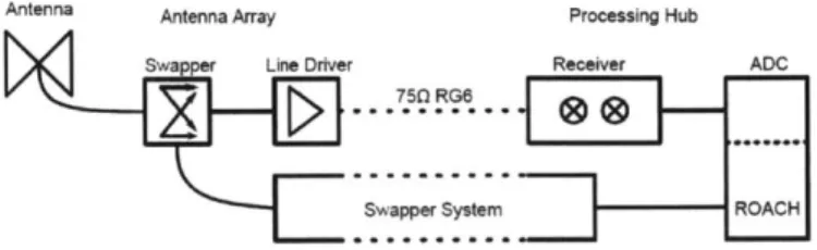
In theory, a very large omniscope can be built following the generalized architecture in Figure 2-1. On the other hand, it is crucial to demonstrate that automatic and precise calibration is possible in real-time using redundant baselines, since the calibration coefficients for each antenna must be updated frequently to allow the FFTs to combine the signals from the different antennas without introducing errors. In this section, we will present our partial implementation of this general design, including both the analog and the digital systems. Because the digital hardware is powerful enough to allow it, the MITEoR prototype correlates all 128 input channels with one another, rather than just a small sample as mentioned in the caption of Figure 2-1. This provides additional cross-checks that greatly aid technological development, where instrumentation may be particularly prone to systematics. This also allows us to explore the question of exactly how often and how finely in frequency we must measure

Analog ADC . Amplification & Filtering Chain F-Engine Fi nFdote FFT Coefficient Calibration I Solver Corner Turner Spatial Gorrelator FFT X-Engines Square Time Time Average Average Post Processing 3D Map Synthesis

3D Map Analysis (Foreground Modeling, Power Spectrum Estimation, Cosmological Model Fitting)

Figure 2-1: Data pipeline for a large omniscope that implements FFT correlator and redundant baseline calibration. First, a hierarchical grid of dual-polarization antennas converts the sky signal into volts, which get amplified and filtered by the analog chain, transported to a central location, and digitized every few nanoseconds. These high-volume digital signals (thick lines) get, processed by field-programmable gate arrays (FPGAs) which perform a temporal Fourier transform. The FPGAs (or GPUs) then multiply by complex-valued calibration coefficients that, depend on antenna, polarization and frequency, then spatially Fourier transform, square and accumulate the results, recording integrated sky snapshots every few seconds and thus reducing the data rate by a factor ~ 109. They also cross-correlate a small fraction of all antenna pairs, allowing the redundant baseline calibration software

[87, 112] to update the calibration coefficients in real time and automatically monitor

the quality of calibration solutions for instrumental malfunctions. Finally, software running on regular computers combine all snapshots of sufficient quality into a 3D sky ball or "data cube" representing the sky brightness as a function of angle and frequency in Stokes (I,Qj,V) [1.67], and subsequent software accounts for foregrounds and measures power spectra and other cosmological observables.