A 3D neuromuscular model of the human ankle-foot complex based on multi-joint biplanar fluoroscopy gait analysis

A 3D Neuromuscular Model of the Human Ankle-Foot

Complex Based on Multi-Joint Biplanar Fluoroscopy Gait

Analysis

David Allen Hill

B.S. Physics Morehouse College, 2010

S.M. Media Arts and Sciences

Massachusetts Institute of Technology, 2012

Submitted to the Department of Media Arts and Sciences in partial fulfillment of the requirements for the degree of

Doctor of Philosophy in Media Arts and Sciences

at the

MASSACHUSETTS INSTITUTE OF TECHNOLOGY June 2018

Massachusetts Institute of Technology 2018. All Rights Reserved.

Signature redacted

A uthor ... ... ... . ... .... ...

Program in Media Arts and Sciences

Signature redacted

May 4,2018

Certified by ...

A ccepted by ...

...

Hugh Herr, Ph.D. Professor of Media Arts and Sciences

and Health Sciences and Technologv

Signature redacted

C)

JUN 272018

MITLibraries

77 Massachusetts Avenue Cambridge, MA 02139

http://Iibraries.mit.edu/ask

DISCLAIMER NOTICE

Due to the condition of the original material, there are unavoidable

flaws in this reproduction. We have made every effort possible to

provide you with the best copy available.

Thank you.

The images contained in this document are of the

best quality available.

A 3D Neuromuscular Model of the Human Ankle-Foot Complex Based on

Multi-Joint Biplanar Fluoroscopy Gait Analysis

David Allen Hill

Submitted to the Department of Media Arts and Sciences

in partial fulfillment of the requirements for the degree of

Doctor of Philosophy in Media Arts and Sciences

at the

MASSACHUSETTS INSTITUTE OF TECHNOLOGY

June 2018

Thesis Committee

Signature redacted

R esearch A dvisor ...

...

Hugh Herr, Ph.D.

Professor of Media Arts and Sciences

Signature redacted

MITMediaLab

T hesis R eader ...

...

Edward Boyden, Ph.D.

Associate Professor of Media Arts and Sciences

MIT Media Lab

Signature redacted

T hesis R eader ...

...

v

_{Brian Umberger, Ph.D.}

Associate Professor of Kinesiology

University of Massachusetts Amherst

Signature redacted

T hesis R eader ...

...

Kevin Moerman, Ph.D.

Post-Doctoral Associate

MIT Media Lab

A 3D Neuromuscular Model of the Human Ankle-Foot Complex Based on Multi-Joint Biplanar Fluoroscopy Gait Analysis

by David Allen Hill

Submitted to the Department of Media Arts and Sciences on May 4, 2018, in partial fulfillment of the

requirements for the degree of

Doctor of Philosophy in Media Arts and Sciences

Abstract

During the gait cycle, the human ankle complex serves as a primary power generator while simultaneously stabilizing the entire limb. These actions are controlled by an intricate interplay of several lower leg muscles that cannot be fully uncovered using experimental methods alone. A combination of experiments and mathematical modeling may be used to estimate aspects of neuromusculoskeletal functions that control human gait. In this research, a three-dimensional neuromuscular model of the human ankle-foot complex based on biplanar fluoroscopy gait analysis is presented.

Biplanar fluoroscopy (BiFlo) enables three-dimensional bone kinematics analysis using x-ray videos and bone geometry from segmented CT. Hindered by a small capture volume relative to traditional optical motion capture (MOCAP), BiFlo applications to human movement are generally limited to single-joint motions with constrained range. Here, a hybrid procedure is developed for multi-joint gait analysis using BiFlo and MOCAP in tandem. MOCAP effectively extends BiFlo's field-of-view. Subjects walked at a self-selected pace along a level walkway while BiFlo, MOCAP, and ground reaction forces were collected. A novel methodology was developed to register separate BiFlo measurements of the knee and ankle-foot complex. Kinematic analysis of bones surrounding the knee, ankle, and foot was performed. Kinematics obtained using this technique were compared to those calculated using only MOCAP during stance phase. Results show that this hybrid protocol effectively measures knee and ankle kinematics in all three body planes. Additionally, sagittal plane kinematics for select foot bone segments (proximal phalanges, metatarsals, and midfoot) was realized. The proposed procedure offers a novel approach to human gait analysis that eliminates errors originated by soft tissue artifacts, and is especially useful for ankle joint analysis, whose complexities are often simplified

in MOCAP studies.

Outcomes of the BiFlo walking experiments helped guide the development of a three-dimensional neuromuscular model of the human ankle-foot complex. Driven by kinematics, kinetics, and electromyography (EMG), the model seeks to solve the redundancy problem, individual muscle-tendon contributions to net joint torque, in ankle and subtalar joint actuation during overground gait. Kinematics and kinetics from BiFlo walking trials enable estimations of muscle-tendon lengths, moment arms, and joint torques. EMG yields estimates of muscle activation. Using each of these as inputs, an optimization approach was employed to calculate sets of morphological parameters that simultaneously maximize the neuromuscular model's

hypothesis that the muscle-tendon morphology of the human leg has evolved to maximize metabolic efficiency of walking at self-selected speed. Optimal morphological parameter sets produce estimates of force contributions and states for individual muscles. This research lends

insight into the possible roles of individual muscle-tendons in the leg that lead to efficient gait.

Thesis Supervisor: Hugh Herr, Ph.D. Title: Professor of Media Arts and Sciences

Acknowledgements

So many have contributed to this process over the last several years. I would like to express a very sincere thank you to the following people:

My research advisor, Hugh Herr. Thank you for all of your insightful advice and direction

throughout the course of my Masters and PhD work. Also, thank you for your patience during my time of leave and family emergencies.

Thesis committee members, Ed Boyden and Brian Umberger, for offering their time, expertise, and enthusiasm in critiquing my project.

Super committee member, Kevin Moerman, for all of your guidance and coaching throughout the thesis. You're the G.O.A.T.

My Biomech research family for being a helpful and inspirational group to work alongside.

Dana Solav for giving your time and advice.

Jared Markowitz for being so selfless and constantly willing to sacrifice time to help others. You are a saint. Thanks for inviting me to the March Madness Bracket Challenge every year and everything else you helped me with since I started at MIT.

Juin-Yih Kuan and David Sengeh for keeping me sane and being all-around good friends. You two were always ears and voices of support when I needed them.

Cameron Taylor for your dedication to science and to Biomech. You continually sacrifice yourself for the greater good of the group... and society. Thanks to Sara Taylor for being just as dedicated.

Bryan Ranger for putting up with me in Autodesk and teaching collaborations over the years.

Lindsey Reynolds for doing everything that you do. Thank you for always being on top of things in the lab. Special shout out to Bevin Lin and Sarah Hunter for being the previous overseers of everything Biomech.

Susan D'Andrea, John Chomack, Erika Giblin, and Beth Brainerd for assisting with data collection. Also, thanks to Bryce Killen for assisting with the MAP Client.

Naomi Dereje and Erica Israel for being amazing UROPs.

Stephanie Ku for lending your amazing artist ability.

MAS staff: Monica, Amanda, Keira, Linda, and Tashi (didn't forget you). Thanks for your

Topper Carew for always checking in and for extending your home during the holidays.

To all the friends that I have gained at MIT and in Boston, thank you for making my life outside of lab enjoyable. Kelvin, Obi, Niaja, Omar, Tsehai, Mareena, Hussein, Uzoma, Jasmine, Postup,

ACME, BGSA, the undergrads, the OGs.

To my friends away from school, thank you for reminding me that there is a life outside of MIT and being encouraging and uplifting when I needed it. Special thanks to my Morehouse Brothers

/ Family that helped me through this time.

Finally, thank you to my family for believing in me. Thank you for being proud and saying good

job no matter what. Thank you to my sisters, Courtney and Adilifu, and brother-in-law, Faruq,

for the long talks. Thank you to my stepfather, Wesley, for stepping in when I needed you. Lastly, thank you to my parents, Paula Henning and David Hill, for being you. You helped me in more ways than you'd ever know. And somehow the distance has brought us closer.

Table of Contents

1.3 Sum m ary of Chapters ... 24

Chapter 2: Background... 25

2.1 Lower Extrem ity Anatomy (Knee, Ankle, & Foot)... 25

2. 1.1 Skeletal Anatomy ... 25

2.1.1.1 Leg Bones and Joints...25

2.1.1.2 Ankle Foot Bones and Joints... 28

2.1.2 M uscular Anatomy... 30

2.2 G ait Analysis ... 34

2.2.1 The Gait Cycle... 34

2.2.2 M etabolic Cost of Transport & Preferred W alking Speed... .35

2.3 Neurom uscular M odeling ... 36

2.3.1 W hat is Neuromuscular M odeling ... . 36

2.3.2 M uscle Activation ... 36

2.3.3 Hill-type M uscle M odel ... 37

2 .3 .3 .1 M u scle F ib er ... 37

2 .3 .3 .2 T e n d o n ... 3 9 2.3.3.3 Model Parameters...40

2.4 Previous Gait M odels ... 40

Chapter 3: Multi-Joint Human Walking Arthrokinematics Using Biplanar Fluoroscopy .43 3.1 Introduction... 43

3.2 M ethods ... 45

3.2.1 Subject Recruitment... 47

3.2.4 Distal Foot M otion Tracking ... 53

33.2.5 Spatial Registration ... 55

3.2.6 Tem poral Registration... 58

3.2.7 Gap Filling... 58

3.2.8 Tibia M atching... 59

3.2.9 Com parison with M OCAP Results ... 61

3.3 Results... 62

3.4 Discussion ... 66

Chapter 4: Three-Dimensional Leg Model Predicts Muscle State and Forces During W alking... 69

4.1 Introduction... 70

4.2 M ethods ... 72

4.2.1 Neurom uscular M odel Overview ... 74

4.2.1.1 M uscle Contraction...74

4.2.1.2 Tendon Strain...77

4.2.1.3 M uscle-Tendon Complex...77

4.2.1.4 Net Joint Torque...78

4.2.2 Experim ental Inputs ... 78

4.2.2.1 Ethics Statement...79

4.2.2.2 Data Collection...79

4.2.2.3 M uscle-Tendon Properties and Joint Dynamics ... 81

4.2.2.4 M uscle Activation ... 84

4.2.3 M uscle-Tendon M orphology Optim ization ... 87

4.2.3.1 M orphological Parameters ... 87

4.2.3.2 Optim ization Overview... 88

4.2.3.3 Objective #1 - Joint Torque M atching... 88

4.2.3.4 Objective #2 - M etabolic Cost M inim ization ... 89

4.2.3.5 Choosing an Optimal Solution ... 89

4.3 Results... 92

4.3.1 Optim al M uscle-Tendon Param eters... 93

4.3.2 Optim al M uscle-Tendon Behavior... 93

4.4 Discussion ... 101

C hapter 5: C onclusion & Future W ork...105

5.2 Future W ork...105

5.2.1 XROM M Gait Analysis...106

5.2.2 Neurom uscular M odeling ... 107

5.2.3 W earable Am bulatory Robotics...109

Bibliography ... 111

A ppendix A : X R O M M N otes...119

Biplanar Fluoroscopy Settings...119

Challenges ... 120

Fluoroscope Positioning...120

Long Bone Tracking with Short Bone Volum es ... 122

Contralateral Lim b Occlusion ... 123

M istim ed or M isplaced Steps ... 125

H andling CT / DICO M Data ... 126

Im age Orientation Patient Correction ... 127

Im age Position Patient Compensation ... 131

Cropping / Cutting DICOM Stacks ... 132

M O CAP M arker Creation for BiFlo M otion Tracking...133

Appendix B: Musculoskeletal Atlas Project (MAP) Client Workflows...135

Filling Subject 1 Tibia with M AP Client...135

Bone M odel Pre-Processing ... 135

W orkflow ... 137

Patient-Specific O pensim M odeling with M AP Client...140

M OCAP Data Pre-Processing ... 140

Bone M odel Pre-Processing ... 140

List of Figures

Figure 2-1: H um an Leg Bones ... 26

Figure 2-2: Tibia and Fibula Bones ... 27

Figure 2-3: A nkle-Foot Bones & Joints ... 29

(A) Ankle-Foot Bones... 29

(B) Ankle-Foot Joints (w/ Bone Nam es)... 29

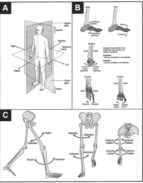
Figure 2-4: Body Planes & Low er Extrem ity Joint M otion... 31

(A) Body Planes... 31

(B) Ankle-Foot M otion ... 31

(C) Leg M otion (Hip & Knee)... .31

Figure 2-5: Leg M uscle A natom y... 32

(A) Anterior View of the Ankle-Foot ... . 32

(B) Posterior View of the Knee, Ankle, and Foot... . 32

(C) Lateral and M edial Views of the Knee, Ankle, and Foot... . 32

Figure 2-6: Phases of the G ait Cycle... 34

Figure 2-7: H ill-type M uscle M odel... 38

(A) M odel Schem atic... 38

(B) M uscle Fiber... 38

(C) Tendon Stress-Strain Curve ... 38

(D) Force-Length Relation... 38

(E) Force-Velocity Relation ... 38

Figure 2-8: Forward Dynamics Neuromuscular Models ... 41

(A) Anderson and Pandy M odel Schematic ... 41

(B) Endo and Herr M odel Schematic... 41

(C) Geyer and Herr M odel Schematic ... 41

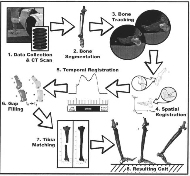
Figure 3-1: Experim ental Protocol ... 46

(1) Data Collection & CT Scan ... 46

(2) Bone Segm entation... 46

(3) Bone Tracking... 46

(6) Gap Filling ... 46

(7) Tibia M atching... 46

(8) Resulting Gait ... 46

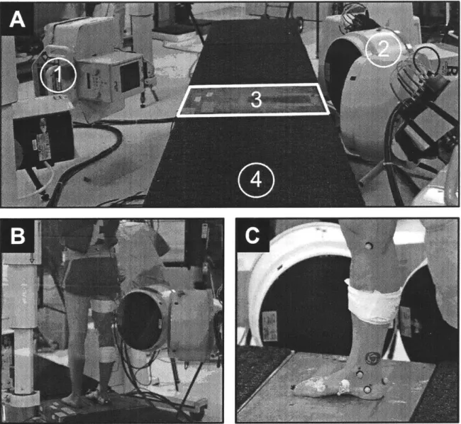
Figure 3-2: Experim ental Setup... 48

(A) BiFlo Experimental Setup... 48

(B) BiFlo Knee Configuration... 48

(C) BiFlo Ankle-Foot Configuration ... 48

Figure 3-3: Bone Segmentation & Three-Dimensional Reconstruction ... 51

(A) CT Scan (Prone Position)... 51

(B) Segmentation M ask Creation ... 51

(C) 3D Bones Overlaid with CT Slices... 51

(D) Reconstructed Bones ... 51

Figure 3-4: Bone M otion Tracking using A utoscoper ... 54

(A) M idfoot Tracking Fluoroscope #1... 54

(B) M idfoot Tracking Fluoroscope #2... 54

(C) M etatarsals Tracking Fluoroscope #1 ... 54

(D) M etatarsals Tracking Fluoroscope #2... 54

(E) Proxim al Phalanges Tracking Fluoroscope #1 ... 54

(F) Proximal Phalanges Tracking Fluoroscope #2 (w/ Reflective M arkers)... 54

(G) Foot Bone Segment Diagram ... 54

Figure 3-5: Spatial Registration... 57

Figure 3-6: Stance Phase Extraction... 58

Figure 3-7: Tibia M atching ... 60

(A) Full Tibia Projections ... 60

(B) Conversion to Single M esh ... 60

(C) Full Tibia Overlay ... 60

(D) Tibia Registration ... 60

(E) Error Analysis... 60

Figure 3-8: Three-Dimensional Knee and Ankle Kinematics ... 64

Figure 3-9: Foot Joint (Sagittal) K inem atics ... 65

Figure 4-1: M odel O verview ... 73

Figure 4-2: Average M uscle-Tendon Lengths ... 82

Figure 4-4: Neural Stimulation & M uscle Activation ... 86

Figure 4-5: Solution Spaces... 90

Figure 4-6: Gastrocnemius and Soleus Fascicle Length Variation ... 91

(A) Gastrocnemius (GAS) Fascicle Length Variation ... 91

(B) Soleus (SOL) Fascicle Length Variation ... 91

Figure 4-7: M uscular M etabolic Cost Breakdown ... 96

Figure 4-8: M odel Torque Predictions... 97

Figure 4-9: Muscle Fascicle, Tendon, & Muscle-Tendon Complex Length Changes... 98

Figure 4-10: Tibialis Posterior Fascicle Length Variation ... 99

Figure 4-11: M uscle Contraction Velocity ... 100

Figure 5-1: Full Leg XROM M Gait Analysis ... 107

Figure 5-2: Three-dimensional Ankle-Foot M odel with M TP Joint ... 108

Figure A-1: Fluoroscope Positioning...121

(A) Poorly Positioned Fluoroscopes ... 121

(B) Well Positioned Fluoroscopes ... 121

Figure A-2: Long Bone Tracking with a Short Bone Volume ... 122

Figure A-3: Long Bone Tracking with a Sufficiently Long Bone Volume ... 123

Figure A-4: Contralateral Limb Occlusion ... 124

(A) Contralateral Limb Occlusion in Camera

1

(B) Contralateral Limb Occlusion in Camera 2...124

Figure A-5: Contralateral Foot Occlusion ... 125

Figure A-6: Poor Foot Placement...126

Figure A-7: DICOM Tags...127

Figure A-8: Orientation Change in M imics...129

(A ) C orrect O rientation ... 129

(B ) Incorrect O rientation ... 129

Figure A-9: Corrected Orientation in M imics...130

Figure A-10: Bone Reconstructions Before & After Orientation Change ... 131

(A) Before Orientation Change ... 131

(B ) A fter O rientation C hange...131

Figure B-1: Bone M odel Pre-Processing ... 136

(A) Partial Tibia Reconstruction with Closed End ... 136

(B) Reconstructed Full Tibia based on Closed M odel... 136

(C) Partial Tibia Reconstruction with Open End ... 136

Figure B-2: Tibia Com pletion W orkflow in M AP Client ... 137

Figure B-3: W orkflow Steps...138

Figure B-4: Final Tibia and Fibula Bone M eshes...139

Figure B-5: Fem ur Pre-Processing...141

(A) Partial Femur Reconstruction with Closed End ... 141

(B) Partial Femur Reconstruction with Open End ... 141

(C) Reconstructed Full Femur based on Closed M odel ... 141

(D) Reconstructed Full Femur based on Open M odel ... 141

Figure B-6: Fem ur Fitting W orkflow in M AP Client...142

Figure B-7: 2-Sided LL Reg Configuration File...143

Figure B-8: O pensim M odel Creation W orkflow ... 144

Figure B-9: Bone Paths File ... 145

Figure B-10: Custom O pensim Block Configuration...145

Figure B-11: O pensim M odel...146

(A) Opensim M odel Bones ... 146

List of Tables

Table 2-1: Ankle-Foot Complex Muscles ... 33

Table 3-1: Subject Information ... 47

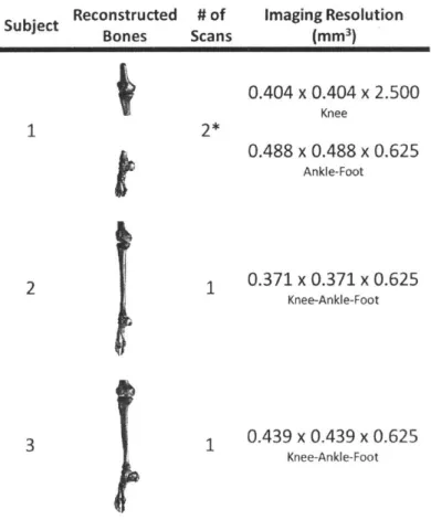
Table 3-2: Imaging Details ... 52

Table 3-3: Bone Visibility in BiFlo ... 63

Table 4-1: Fixed Muscle Parameters... 76

Table 4-2: Subject Information ... 79

Table 4-3: Optimization Parameter Bounds... 88

Table 4-4: Optimization Results... 93

Table 4-5: Optimal Morphological Parameters for Each Subject ... 94

Table 4-5 (Cont.): Optimal Morphological Parameters for Each Subject... 95

Table A-1: Biplanar Fluoroscopy Settings for Subject 1...119

List of Terms

Neuromuscular - Relating to both nerves and muscles.

Ankle-Foot Complex - The segment of the leg comprised of the ankle joint and foot structure. XROMM - X-ray Reconstruction of Moving Morphology, abbreviated as XROMM, is a 3D imaging technology for visualizing skeletal motion in vivo.

Biplanar Fluoroscopy (BiFlo) - Fluoroscopy, commonly referred to as videoradiography or simply x-ray movies, is an imaging technique that uses x-rays to obtain real-time moving images of the interior of an object. The added term, biplanar, refers to the extension of this technique to two planes for capturing movement in three dimensions.

Ionization Radiation - Radiation that carries enough energy to free electrons from atoms or molecules, thereby, ionizing them. Two types of electromagnetic waves ionize atoms: x-rays and gamma rays.

Biomechanics - The study of the structure and function of biological systems by means of the methods of mechanics.

Gait Analysis - The study of walking or other types of ambulation.

Energetics - A branch of mechanics that deals primarily with energy and its transformations. Arthrokinematics - Angular movement of bones in the human body with regard to joint surfaces.

Dynamics - The branch of mechanics concerned with the motion of bodies under the action of forces.

Sagittal Plane - The anatomical plane which divides the body into left and right parts. Proximal - Situated nearer to the center of the body or the point of attachment.

Chapter

1

Introduction

Bipedal locomotion is the highly optimized and efficient process by which humans transport themselves from one location to another. Extensive studies of human locomotion have provided scientists with a deep understanding of the behavior of the leg and its segments during gait. Many characteristics of human gait can be quantified and evaluated using non-invasive technology; such as optical motion tracking, goniometers, force sensors, inertial measurement units, and various other sensors. These have helped uncover aspects of the current understanding of human gait: the gait cycle, individual joint contributions, muscle activation and timing estimates, and a functional description of the upper body during locomotion.

However, the complexities of the human body and challenges of performing invasive procedures make it difficult to study some of the underlying functions that govern the behavior of the body during dynamic actions. In the case of human locomotion, one can obtain an in-depth description of externally observable phenomena using non-invasive techniques, as discussed previously, but reliable methods for evaluating internal behavior, such as that of the musculoskeletal and nervous systems, present a much bigger challenge. Mathematical modeling is one credible approach for evaluating such behavior.

Mathematical modeling offers insight into systems that are difficult to study empirically, allowing one to uncover the various nuances of the system and predict its behavior under large sets of conditions. It is this ability to reveal the difficult to measure, intrinsic attributes of a system that make modeling useful for analyzing human locomotion. One can derive equations that relate the difficult-to-measure, intrinsic attributes of the human body to the

simple-to-Put differently, one can use easily measured properties of human gait to infer intrinsic behavior of the body. This permits scientists to study how attributes such as muscle state, force, activation, and energetics progress during the gait cycle. It should be noted, however, that mathematical models are often based on various assumptions and idealized conditions that make them approximations of reality and imperfect representations of the actual systems.

For example, gait models commonly rely on optical motion tracking, cadaver studies, and external body segment measurements to define and/or evaluate geometry and arthrokinematics. As previously stated, mathematical gait modeling is a means to analyze internal attributes of the human body that are difficult to measure non-invasively and during dynamic tasks. Medical imaging offers an empirical approach to the non-invasive assessment of internal geometry, which can replace the need for cadaver studies and external segment measurements. Further, optical motion tracking uses external reflective markers to approximate bone positions. Dynamic radiography allows users to observe internal bone motion without the need for markers or any invasive procedures. These imaging techniques may be used to supplement modeling tasks.

This research project aimed to develop two methodologies for analyzing internal behavior of the body during gait: (1) a novel approach to multi-joint gait analysis using biplanar fluoroscopy (BiFlo) and (2) a three-dimensional, neuromuscular, inverse dynamics model of human ankle complex behavior during gait. (1) BiFlo is a procedure for obtaining 3D direct bone kinematics using essentially x-ray videos. This study featured a set of level-ground walking trials at a preferred walking speed (~1.3 m/s) that collected BiFlo data in tandem with optical motion capture. Knee, ankle, and foot BiFlo data were compared against optical motion capture to observe differences in arthrokinematics. (2) The mathematical model is completely biophysical

-incorporating each of the major muscle-tendons that govern three-dimensional motion of the ankle joint. BiFlo kinematics from (1) served as inputs to the inverse dynamics model, which yielded predictions of individual muscle-tendon state and joint torque contributions. This research offers understanding of the musculoskeletal and nervous functions necessary to produce economical human walking.

This research project addresses the following questions:

1) Is Biplanar Fluoroscopy a viable alternative to conventional Motion Capture for

multi-joint gait analysis?

2) Can a neuromuscular walking model be derived that captures three-dimensional dynamics of the human ankle at a metabolic cost consistent with literature?

Hypothesis

HI: We hypothesize that muscle-tendon morphologies of the muscles comprising the ankle-foot complex have evolved to minimize the metabolic cost of walking at self-selected speed.

1.1

Thesis Objectives

This thesis has the following aims:

1) Conduct Biplanar Videoradiography

foot bone motion.

(XROMM) walking trials to track knee, ankle, and

2) Develop a neuromuscular walking model that captures three-dimensional dynamics of the ankle-foot complex and predicts muscle-tendon morphology and muscle state.

The outcomes of this thesis are a novel methodology for multi-joint gait analysis/direct bone motion tracking using biplanar fluoroscopy and a neuromuscular model of human walking that predicts three-dimensional joint dynamics and individual muscle-tendon torque contributions.

This work is an investigation of the coordinated efforts of the musculoskeletal and nervous systems to produce efficient gait. In creating a model that realistically simulates human walking, predicting muscle-tendon morphology and fascicle dynamics, one can begin to resolve the complex functions of the internal structures that control legged locomotion. This could prove to be critical in the sciences of rehabilitation and augmentation, as it allows practitioners to gain a deeper view of what may be occurring internally to cause common medical conditions and offers insight into how these conditions, and body function in general, may be improved with technology to meet or exceed normal ability. This research will contribute to new experimental and computational approaches to gait analysis, rehabilitation, and augmentation.

1.3

Summary of Chapters

Chapter 2 outlines the previous work that motivates and is critical for understanding this thesis. It covers gait analysis, knee-ankle-foot anatomy, muscle physiology, and gait modeling.

Chapter 3 details the novel gait analysis methodology proposed in this study. A thorough description of the biplanar fluoroscopy data collection and analysis protocol can be found here.

Chapter 4 describes the modeling component of the work. Included is a detailed description of the proposed neuromuscular model, along with outcomes, validation, and discussion.

Chapter 5 concludes the thesis - summarizing its findings and offering suggestions for future work.

Chapter 2

Background

This chapter outlines previous studies relevant for understanding and conducting this research. It begins with a description of human anatomy, focusing on the knee, ankle, and foot, as these body segments are the focal points of this work. An introduction to human gait analysis follows, including a section on the current state of gait analysis technology. Finally, the chapter closes with an overview of human gait modeling.

2.1

Lower Extremity Anatomy (Knee, Ankle, & Foot)

A description of human leg anatomy is presented below. This thesis focuses solely on the knee,

ankle, and foot. As such, the anatomy covered in this section will only detail those bones and muscles spanning the knee joint, ankle joint, and foot structure. No thigh muscles will be presented.

2.1.1 Skeletal Anatomy

2.1.1.1 Leg Bones and Joints

Four bones make up the human leg (plus thigh): femur, tibia, fibula, and patella. The femur, the sole bone of the thigh, is the largest, longest, and strongest bone in the body. Proximally, the femur connects with the pelvis at its acetabulum cup to form the hip joint [1]. Distally, the femur

bearing bone of the leg below the knee. Commonly referred to as the shinbone or shankbone, the

tibia is the larger of the two major bones below the knee and forms the connection between the

knee and the ankle. The patella, or kneecap, is critical to knee extension. Its primary purpose is

to increase the lever arm on which knee extensors act on the knee, thus enhancing torque

production.

Coxal bone:

Acetabulum

Pubis

Head

Ischium

Greater

trochanter

Lesser

trochanter

4-

Femur

Medial

Patella

condyle

Head of fibula

Tibia

-Fibula

7 Tarsals

5 Metatarsals

14 Phalanges

Figure 2-1: Human Leg Bones. The head of the femur and the acetabulum of the

pelvis form the hip joint. The distal femur, proximal tibia, and patella form the

knee joint. Source: https://www.amazecraze.com/bones-in-the-body

Unlike the thigh, the region below the knee is comprised of two bones: the tibia and fibula.

While the proximal end of the tibia connects with the femur and patella to form the knee joint,

the proximal end of the fibula originates just below the knee joint and runs laterally alongside the

tibia. The distal ends of the tibia and fibula are a part of the ankle joint. The fibula, also called

the calfbone, is one of the slenderest long bones in the body [1]. In contrast with the tibia, the

fibula is not weight bearing. Its primary purpose is ankle stability.

Lateral

Head

of

Proxmal

tibiobtdar

joint

Distal

tibijoibular

jOnt

Fibula

Anterior view Posterior view

Figure 2-2: Tibia and Fibula Bones. The head of the fibula is located toward the

back of the tibia and just below the knee. The fibula is located on the lateral side

of the tibia. Distal ends of the tibia and fibula are a part of the ankle joint. The

lateral and medial malleoli are the bony prominences on either side of the ankle.

The medial malleolus is on the distal end of the tibia. The lateral malleolus is on

which the tibia and fibula attach to one another on either end of each bone. Limited motion occurs at the joints [2]. Source: http://encyclopedia.lubopitko-bg.com/PelvicBones.html

2.1.1.2 Ankle Foot Bones and Joints

What is commonly referred to as the ankle, is actually three joints: the inferior tibiofibular joint, talocrural joint, and subtalar joint. Four bones comprise these joints. They are the tibia, fibula, talus, and calcaneus. A connection between the distal ends of the tibia and fibula form the inferior tibiofibular joint. The inferior tibiofibular joint's primary function is ankle stability, preventing excessive joint rotation and bone translation [2]. Limited range of motion is displayed at the joint. Note that the inferior tibiofibular joint is separate from the superior tibiofibular joint, though they both serve as connections between the tibia and fibula. However, the joints appear on opposite ends of the bones. The inferior tibiofibular joint is located distally, at the ankle, while the superior tibiofibular joint is located proximally, closer to the knee.

Often, the term "ankle' refers to the talocrural joint. This joint is located at the intersection of the tibia, fibula, and talus bones. The talocrural joint is characterized by its ability to plantar flex and dorsiflex the foot. This joint exhibits the largest range of motion of the three "ankle" joints, primarily moving in the sagittal plane. During the gait cycle (see Section 2.2.1 of this thesis), for example, the average human exhibits a range of motion in the talocrural joint of approximately

300 [3]. For the duration of this thesis, any mention of the term "ankle" will refer to the talocrural joint.

The subtalar, or talocalcaneal, joint is found at the contact point of the talus and calcaneus bones. The subtalar joint permits inversion and eversion of the foot. It has a much smaller range of motion than the talocrural joint. During the gait cycle, coronal plane motion of the foot has been shown to have about a 10' range of motion [3].

The human foot is highly complex. Comprised of 26 bones and 33 joints (20 actively articulated), foot structure closely resembles that of the hand, but sustained high loads, relative to the hand,

make it much stronger but less dexterous [1]. Foot bones are characterized as one of three

different types: tarsal bones, metatarsal bones, and phalanges. There are 7 tarsal bones. Tarsal

bones are located toward the rear of the foot. They are the talus, calcaneus, navicular, cuboid,

and 3 cuneiforms. Toward the forefoot, five metatarsals and 14 phalanges are found. Phalanges

are categorized into proximal, middle, and distal phalanges. In addition to the subtalar joint,

several other joints exist in the foot. This research focuses mostly on the metatarsophalangeal

(MTP) joints, the joints between the metatarsals and distal phalanges, but each of the joints in the

foot play a critical role in its health and function, whether it's stability or actuation.

Tamd Cubid Tarsa

=M

oe

Figure 2-3: Ankle-Foot Bones & Joints. (A) The human foot includes 26 bones

and 33 joints. All 26 bones, along with the distal ends of the leg bones, are visible.

The tibia and fibula combine with the talus to form the talocrural joint. Foot bones

are subdivided into 3 types of bones: tarsal bones, metatarsal bones, and

phalanges. Source: http://encyclopedia.lubopitko-bg.com/PelvicBones.html. (B)

Several joints are present in the foot. The subtalar joint is located at the

intersection of the talus and calcaneus. The metatarsophalangeal joint, called

Mediotarsal joint here, appears at the intersection of the metatarsals and distal

phalanges. Interphalangeal joints are located between the phalanges (distal,

middle, and proximal). The Lisfranc's joint is located between the anterior

portions of the tarsal bones and the metatarsals. Additionally, several other joints

appear between the intersections of each small foot bone; including the

naviculocuneiform joints, talonavicular joint, and calcaneocuboid joint. Source:

http://humananatomylibrary.com/foot-anatomy-bones-joints/foot-anatomy-bones-joints-tag-foot-anatomy-bones-and-joints-human-anatomy-diagram

2.1.2 Muscular Anatomy

Over 40 muscles are present in the human leg [1]. Each plays a very specific role in total leg motion, joint orientation, posture, and stability. Muscles are typically characterized by the body motions which they produce; that is, whether they extend, flex, adduct, abduct, rotate internally, or rotate externally the body segment on which they act. These motions can be seen more clearly in Fig 2-4.

Flexors are muscles that generate a joint angle decrease in the sagittal plane [3]. They are opposed by extensors, which generate a joint angle increase in the sagittal plane, generally resulting in the straightening of the limb. Abductors are muscles that draw the limb away from the sagittal plane. This motion occurs in the coronal plane. Adductors oppose this motion, drawing the limb toward the sagittal plane. Each joint has its own set of muscles and/or tendons that contribute to its motion, in forms similar to that previously described. Last, internal and external rotation are transverse plane motions that bring the limb toward the center of the body and away from the center of the body, respectively. Many times, a single muscle will contribute to joint mobility in more than 1 plane. Further, a single muscle may also contribute to motion about more than one joint. This type of muscle is called biarticular. A muscle that only actuates a single joint is called monarticular.

This research focuses on those muscle-tendons that actuate the ankle-foot complex. Therefore, only muscles that fit this constraint are discussed in this section. The biarticular gastrocnemius drives motion at both the knee and ankle, as a primary ankle plantarflexor and knee flexor. It performs the second most plantarflexion torque, next to the soleus, with which it is attached to the calcaneus via the shared Achilles tendon, the thickest in the body. Figure 2-5 shows the rest of the ankle-foot muscle-tendons, along with their tendon insertion points. Muscles surrounding the foot have complex wrappings and attachments that contribute to its unique motion and mechanical attributes. Table 2-1 displays muscle contributions to motion at the major joints in the ankle-foot.

Left

x4

U

Il::

EMM~ &rdUw SWd ticbn

LEtWb WW

EwmO* ("M

Exeromm

Etembn reao

Figure 2-4: Body Planes & Lower Extremity Joint Motion. (A) The sagittal, frontal, and transverse anatomical planes each transect the human body for the purpose of describing anatomical landmarks and the nature of body motions. The frontal plane is often referred to as the coronal plane. (B) Motion of the human ankle-foot is described. (C) Motion of the human leg (hip and knee) is described.

I MOW

A" To"

FWdon

A

sapodarlnso %WWsorrenkcW

LateralMallolofl KA&

Fbum longus Wedon

Fbufttrs bava landon ExWnortA brais Base of W1n motatsm

atensorbdlo - WWIormums

Abdulortmnmpedis -Dorsal oterssatpOdis

Dorsal (NOW panwSn of and bos

p

"X

Head of ft"

-

I-- ptanm'

Oalmam lateral h&W

T"wipoAr

Ttrahe"e

F.hOWsgus -4

Cakcanus

- Fibimals lu a t bu

Fibulans brons twndon

Fla.r diorm ngu V"Wn

Fburnd erbus

ralmaculim Psas*

or ha"oru3

E sndoom Tobls anwiDr

Flari Fibulad brawls

&t igdo iloru Jogus tW O s

- Renaa fibors TbWh podwior Flaor dgitrun longus Flexo t~akicm of %WO K Akhos) lno

Figure 2-5: Leg Muscle Anatomy. (A) Anterior view of the ankle-foot. (B) Posterior view of the knee, ankle, and foot. (C) Lateral and Medial views of the knee, ankle, and foot. Major muscles that control motion at the talocrural, subtalar, and metatarsophalangeal joints are displayed. Note the muscles in the diagram beginning with Fibularis. In this thesis, Fibularis will be interchanged with Peroneus. Source: https://musculoskeletalkey.com/I 1-muscles-of-the-leg-and-foot/#cesec I

solaus

-Fibulam kewgs

(ACMIh) landon

Relative Torque

(% Soleus)

Soleus 100.0%

Gastrocnemius 68.0%

Flexor Hallucis Longus 6.1%

Peroneus Longus 2.4%

Tibialis Posterior 1.8%

Flexor Digitorum Longus 1.8%

Peroneus Brevis 1.0% Plantaris Ankle Dorsiflexors Relative Torque (% Soleus) Tibialis Anterior 6.9%

Extensor Digitorum Longus 2.7%

Extensor Hallucis Longus 1.1%

Peroneus Tertius

-Relative Muscle Leverage

(% Tibialis Posterior)

Tibialis Posterior 100%

Tibialis Anterior 63%

Flexor Hallucis Longus 51%

Soleus 43%

Relative Muscle Leverage

(% Tibialis Posterior)

Peroneus Longus 108%

Peroneus Brevis 100%

Extensor Digitorum Longus 92%

Extensor Hallucis Longus 23%

Peroneus Tertius Flexor Digitorum Longus

Flexor Hallucis Longus Big Toe Flexion

Extensor Hallucis Longus Big Toe Extension

Extensor Digitorum Longus

Table 2-1: Ankle-Foot Complex Muscles [3]. Ankle plantar flexors and

dorsiflexors are presented in the order of their torque contribution. The values are

normalized by soleus torque, which performs the largest magnitude of torque on

the joint. Subtalar inverters and everters are presented in the order of their

individual leverage on the subtalar joint. Each muscle's leverage is compared to

that of the tibialis posterior muscle, which is the biggest contributor to subtalar

joint inversion. Some muscles are not reported in [3], as indicated by

'-'

in the

2.2

Gait Analysis

This section discusses key aspects of gait analysis. It will introduce commonly used concepts and terminology.

2.2.1 The Gait Cycle

Human walking can be broken down into recurrent periods known as gait cycles. Each period, or gait cycle, is bounded by consecutive heel-strikes of a single leg.

Gait cycle 100%

Stance phase (St) ca. 60% Swing phase (Sw) ca. 40%

0% 0-10% 10-30% 30-50% 50-60%

initial loading mid terminal pre-Sw

contact response St St

Single _{support P} ,Double SUPPOrP

60-73% 73-87% 87-100%

initial mid terminal

Sw Sw Sw

Toe off

Figure 2-6: Phases of the Gait Cycle [3]. Initial contact and heel-strike are often

used interchangeably. Heel-strike signifies the beginning of stance and the end of

swing. Toe-off signifies the end of stance and the beginning of swing.

One gait cycle, heel-strike to heel-strike, is often referred to as a stride. In studies involving gait,

actions are often referenced as a percentage of the total gait cycle, from 0% (first heel-strike) to

100% (second heel-strike). The gait cycle is divided into two main segments: stance phase, when

the foot is contacting the ground, and swing phase, when the foot is in the air. When walking on

level ground at a moderate pace, stance accounts for approximately 60% of the gait cycle; whereas, swing accounts for 40%. Human walking is characterized by a period of stance known as double support, in which both feet are simultaneously in contact with the ground. This is due to the fact that each leg's stance accounts for over 50% of its gait cycle. The opposite period of stance is single support, in which one leg supports the entire body's weight. Stance and swing can be further subdivided to more clearly assess the behavior of the lower extremities during the gait cycle. Figure 2-6 is a clear depiction of each gait cycle phase [3].

The gait cycle is a crucial part of this, and any other, gait related study, as walking is typically examined with respect to its cycle. As such, many of the plots to follow will be presented as functions of gait cycle percentage, as opposed to time.

2.2.2 Metabolic Cost of Transport & Preferred Walking Speed

Metabolic Cost of Transport (MCOT) is a measure of the metabolic energy required for an animal to transport a unit of its own body weight a unit of distance. The quantity is expressed by the following equation [4]:

EM

MCOT = (2.1)

where Em is metabolic energy expenditure, m is body mass, g is Earth's gravitational pull, and d is distance traveled. MCOT is a dimensionless quantification of energy efficiency. It includes the basal metabolic cost, which is the baseline energy expenditure associated with maintaining bodily function at rest.

Metabolic energy expenditure has a quadratic relation to walking velocity [4], [5]. As such, the plot of metabolic cost of transport versus walking velocity forms an upward opening parabola with a speed at which an MCOT minimum occurs. For many, this minimum occurs around 1.33

tends to occur at a speed very close to an individual's self-selected, or preferred, walking speed [4]. This has led to the belief that humans modulate their gait to minimize MCOT.

2.3

Neuromuscular Modeling

Key aspects of neuromuscular model development are described. The section begins with a description of neuromuscular modeling. An explanation of electromyography, a common technique used to analyze muscle activity, follows. The section concludes with an overview of a

common mathematical model of muscle and tendon physiology.

2.3.1 What is Neuromuscular Modeling

Neuromuscular modeling refers to the practice of modeling movement produced by the musculoskeletal system as controlled by the nervous system [6]. Two types of models exist: forward dynamics and inverse dynamics. Forward dynamics models are driven by neural commands and output joint kinematics. Alternatively, inverse dynamics models start with joint kinematics and external forces and produce joint kinetics and muscle forces. Both approaches come with a unique set of challenges arising from limitations in technology and various assumptions necessary during the process.

2.3.2 Muscle Activation

Many neuromuscular models require neural commands as inputs. Neural commands are the magnitude of muscle activation. Often, these values are extracted from processing electromyographic (EMG) signals. Electromyography is a technique used to evaluate electrical activity produced by skeletal muscle. In their raw form, EMG signals are voltages with both positive and negative values that vary magnitude based on the amount of muscular effort required to accomplish a given task. However, EMG signals must be transformed into muscle activation before use in neuromuscular models.

Muscle activation values take a different form than raw EMG signals. These values typically fall between a range of 0 and 1, representing the normalized magnitude of muscle activation required to carry out a task at any given point in time. Neuromuscular models are highly vulnerable to discrepancies in muscle activation, and thus EMG. This is one of the primary shortcomings of many neuromuscular models, as EMG exhibits substantial variability, especially in magnitude. This variability is most often due to differences in hardware, equipment settings, electrode placement, and several biological attributes [6]. EMG recordings are usually normalized by maximum muscle contractions to account for this variability.

2.3.3 Hill-type Muscle Model

Converting muscle activations to muscle forces is a non-trivial process. It requires a model of muscle contraction dynamics that accepts neural commands, along with other muscle attributes, and transforms them into forces and/or torques. Several of these models exist [7]-[10]. However, many include highly complex differential equations that are computationally intensive to solve. Hill-type muscle models, proposed by A.V. Hill in 1938 [10], are most widely used in neuromuscular models containing many muscles, as they are less computationally expensive and reasonably explain the behavior of muscle.

Hill-type models represent the viscoelasticity of muscle-tendon units (MTU) by placing muscle fiber in series with tendon, as shown in Figure 2-7A. MTUs have a net length and velocity determined by the orientation of the joints they span. However, separate muscle and tendon attributes are more difficult to ascertain.

2.3.3.1 Muscle Fiber

Muscle fiber is represented in Hill-type MTUs as a contractile element in parallel with an elastic element (Figure 2-7B). The contractile element actively generates force; whereas, the elastic (passive) element represents the elasticity of muscle tissue and resists over-stretching of the muscle.

-- U. -- -... -I

A

._/2

.U-CowVtl

I

ET

r

F

0.51.

1.

Figure 2-7: Hill-type Muscle Model. (A) The Hill-type muscle model

configuration is meant to represent muscle fiber in series with tendon. Muscle fiber is attached to tendon at an angle, 0. (B) Muscle fiber includes a contractile element in parallel with a passive elastic element. (C) Normalized stress-strain curve of tendon. The shaded black region of the curve is non-linear. The linear region follows. (D) Force-length relation of muscle. The active component of muscle exhibits a bell-shaped relation with an optimal at the length,

4e.

The force generated by the contractile element of the muscle fiber, Fee, is given by the equation:

Fee (t) = a(t)f1(Ice (t))fv(Vee (t))F (2.2)

where a is muscle activation,

fi

f,

is time [6]. The total force generated by muscle fiber, F, is given by:

Fm(t) = Fce(t) + FPe(t) (2.3)

where Fe is the force generated by the passive, parallel element of muscle fiber.

As shown above, muscle force, Fle, is a function of muscle length and velocity. The contractile element of muscle fiber produce a peak force at an optimal length. Above and below this length, a less than optimal force is produced, yielding a bell-shaped force-length relationship, as in Figure 7D. Muscle force and velocity are related to one another in the form shown in Figure

2-7E. As muscle contractions occur more rapidly, less force is generated. The combined efforts of

these two relations contribute to overall muscle force generation by muscle fiber.

2.3.3.2 Tendon

If muscles are the actuators that enable motion of the skeleton, then tendons are the transmissions

that transmit force between muscle and bone. Tendons are non-linear elastic structures connecting each muscle to the bone it actuates. As such, any force that passes through the muscle must also pass through the tendon, and vice versa. Muscle and tendon are connected to one another at an angle, known as the pennation angle, which changes with time [6]. This angle has a direct impact on the amount of force transferred through the tendon.

Generally, tendon force is a function of tendon length. The force-length relation often takes on a form similar to that in Figure 2-7C. This relation is based on the tendon's elastic properties. The tendon's slack length determines at what length tendon begins transmitting force. Below the slack length no load is carried. Force is not generated in the tendon until the slack length is exceeded.

2.3.3.3 Model Parameters

Several parameters dictate the properties of neuromuscular models. For Hill-type models, physiological parameters include maximum isometric muscle force, optimal muscle fiber length, and tendon slack length. Many other physiological parameters exist. Each parameter helps define how individual muscles and tendons react to state changes. Further, inverse dynamics calculations are particularly vulnerable to muscle-tendon moment arms and body geometry. Torque contributions are highly sensitive to these values. Researchers use a variety of methods to determine model parameters. Two of the most common methods are cadaver studies [6], [12] and optimization methods [13].

2.4

Previous Gait Models

Mathematical models have been used to describe several attributes of human gait. Simple inverted pendulum and spring-mass systems have been shown to replicate the body's center of mass trajectory for walking and running [14], [15]. The same inverted pendulum model has been expanded to represent certain energetic aspects of walking, leading to implications about leg behavior and energy transfer during normal gait actions and how those attributes vary under altered conditions [16]. Additional complexities allowed these once simple models to more closely resemble actual human biology. For example, knee and ankle joints, along with feet, were added to the inverted pendulum [17].

Neuromuscular models are another approach to studying human walking. These models incorporate elements of mechanical and neural interactions of the musculoskeletal system [18],

[19]. Neuromuscular walking models allow one to uncover properties of individual muscles and

tendons, often using Hill's widely adopted model of human muscle [10] and some associated methods for estimating metabolic cost [20].

One of the current shortcomings of neuromuscular models is that most overestimate the energy required to transport the body from one location to another, or metabolic cost of transport

(MCOT) [21]. Two of the most advanced models, Geyer and Herr [18] and Anderson and Pandy

[19], predict reasonable kinematics but high MCOT values compared to experimental data

recorded at preferred walking velocity [21]. Alternatively, Endo and Herr hypothesized that the

majority of muscles in the leg produce force isometrically, thus exploiting the elastic properties

of muscle-tendons [22]. Given this hypothesis, they were able to develop a model that predicted

realistic MCOT. However, this model is not completely biophysical, as it simulates isometric

muscle with clutch-springs. Schematics for all three models discussed in this paragraph are

shown in Figure 2-8.

Knee Flewm Knee Extemor

Ankle-Knee Posterior

Ankle Plantar Flexor Anide Domiflexor

AchMIles Tendon

AAA

three-dimensional model of the body with 23 degrees-of-freedom actuated by 54

musculotendinous units. (B) Endo and Herr [22] is a two-dimensional model of the leg that operates in the sagittal plane and includes a mixture of clutch-springs and muscle-tendon units. Clutch-springs represent isometric muscle activity. (C) Geyer and Herr [18] is a two-dimensional model of the body that operates in the sagittal plane. It includes 7 musculotendinous actuators per leg and is purely reflex driven.

Motivated by the previous studies, Krishnaswamy et al. [23] set out to develop an inverse dynamics approach for determining individual muscle-tendon torque contributions at the ankle during walking. This neuromuscular model used gait kinematics to run inverse calculations of muscle-tendon dynamics and energetics for three muscles: the gastrocnemius, soleus, and tibialis anterior. The model was shown to closely match experimental ankle torques and predicted muscle-tendon morphology and energetics for each modeled muscle. Eventually, this model was pushed forward by Markowitz and Herr [13] to include the entire leg and was shown to predict realistic metabolic cost of transport and optimal muscle-tendon parameters for 10 subjects. The Markowitz and Herr model was two-dimensional (sagittal plane motion only) and included 9 muscles per leg.

Chapter 3

Multi-Joint Human Walking Arthrokinematics

Using Biplanar Fluoroscopy

Biplanar fluoroscopy (BiFlo) enables three-dimensional bone kinematics analysis using x-ray videos and bone geometry from segmented CT. Hindered by a small capture volume relative to traditional optical motion capture (MOCAP), BiFlo applications to human movement are generally limited to single-joint motions with constrained range. Here, a hybrid procedure is developed for multi-joint gait analysis using BiFlo and MOCAP in tandem. MOCAP effectively extends BiFlo's field-of-view. Three healthy adult subjects walked at a self-selected pace along a level walkway while BiFlo, MOCAP, and ground reaction forces were collected. A novel methodology was developed to register separate BiFlo measurements of the knee and ankle-foot complex. Kinematic analysis of bones surrounding the knee, ankle, and foot was performed. Kinematics obtained using this technique were compared to those calculated using only MOCAP during stance phase. Results show that this hybrid protocol effectively measures knee and ankle kinematics in all three body planes. Additionally, sagittal plane kinematics for select foot bone segments (proximal phalanges, metatarsals, and midfoot) was realized. The proposed procedure offers a novel approach to human gait analysis that eliminates errors originated by soft tissue artifacts, and is especially useful for ankle joint analysis, whose complexities are often simplified in MOCAP studies.

Conventional methods often rely upon two or more cameras to triangulate the three-dimensional position of a body within a volume by using externally attached markers to indicate joint centers and critical landmarks. Resolving the intersection points of the markers between cameras allows one to extract the movement of vital segments [24]-[27]. Optical motion capture (MOCAP) tends to be highly versatile, yielding accurate kinematic data for a variety of human motions [28]-[30]. However, MOCAP is vulnerable to errors due to soft tissue artifact [31]-[34], particularly at moments of impact, and has difficulty precisely quantifying small joint motion, such as that of the complex articulating structures of the foot and secondary knee angles (ab/adduction and internal/external rotation).

Fluoroscopy offers an alternative method for human motion tracking. One can describe this method as x-ray video, and it exhibits some key differences from traditional MOCAP techniques. Fluoroscopy enables in vivo examination of internal tissues and deep structures of the body during dynamic activities [35]. This examination of direct bone motion, rather than external marker motion, eliminates motion artifacts from marker drift [36]. The resulting fluoroscopic videos allow one to observe the various articulations of bones relative to one another. Previous researchers have used this technique to analyze shoulder motion [37], [38], evaluate knee kinematics during a range of activities post-ACL reconstruction [39], [40], and examine soft tissue artifacts in patients with total knee arthroplasty [41].

Biplanar Fluoroscopy (BiFlo) captures three-dimensional movement using two orthogonally placed fluoroscopes. In 2010, researchers at Brown University published a methodology that uses BiFlo to quantify pig mandible movements with high-precision [35]. The procedure involved overlaying three-dimensional bone reconstructions obtained from segmented CT scans with biplanar x-ray videos and extracting the three-dimensional motion of the bones relative to each other. In the years following, this procedure was adapted to study human mobility. A study of the jump-cut maneuver found that knee joint rotations and translations could differ by up to

150 and 28 mm when comparing MOCAP to BiFlo around moments of impact [36].

A drawback to BiFlo is the small capture volume - approximately 6,000 cm3 or the size of a soccer ball - in comparison to traditional MOCAP [35]. Confined to this relatively small field of