HAL Id: hal-00470529
https://hal.archives-ouvertes.fr/hal-00470529
Submitted on 21 Apr 2010
HAL is a multi-disciplinary open access
archive for the deposit and dissemination of
sci-entific research documents, whether they are
pub-lished or not. The documents may come from
teaching and research institutions in France or
abroad, or from public or private research centers.
L’archive ouverte pluridisciplinaire HAL, est
destinée au dépôt et à la diffusion de documents
scientifiques de niveau recherche, publiés ou non,
émanant des établissements d’enseignement et de
recherche français ou étrangers, des laboratoires
publics ou privés.
Latin Hypercube Sampling of Gaussian random field for
Sobol’ global sensitivity analysis of models with spatial
inputs and scalar output
Nathalie Saint-Geours, Jean-Stéphane Bailly, Christian Lavergne, Frédéric
Grelot
To cite this version:
Nathalie Saint-Geours, Jean-Stéphane Bailly, Christian Lavergne, Frédéric Grelot. Latin Hypercube
Sampling of Gaussian random field for Sobol’ global sensitivity analysis of models with spatial inputs
and scalar output. Accuracy 2010, Jul 2010, Leicester, United Kingdom. pp.81-84. �hal-00470529�
Latin Hypercube Sampling of Gaussian random field
for Sobol’ global sensitivity analysis of models with
spatial inputs and scalar output
Nathalie Saint-Geours
Jean-Stéphane Bailly
AgroParisTech, UMR TETIS F-34093, Montpellier, Francesaintge@teledetection.fr, bailly@teledetection.fr
Frédéric Grelot
Cemagref, UMR G-EAU F-34093, Montpellier, Francefrederic.grelot@cemagref.fr
Christian Lavergne
Mathematics and Modelling Institute of Montpellier Montpellier 3 University
Montpellier, France Christian.lavergne@univ-montp3.fr
Abstract — The variance-based Sobol' approach is one of the
few global sensitivity analysis methods that is suitable for complex models with spatially distributed inputs. Yet it needs a large number of model runs to compute sensitivity indices: in the case of models where some inputs are 2D Gaussian random fields, it is of great importance to generate a relatively small set of map realizations capturing most of the variability of the spatial inputs. The purpose of this paper is to discuss the use of Latin Hypercube Sampling (LHS) of geostatistical simulations to reach better efficiency in the computation of Sobol’ sensitivity indices on spatial models. Sensitivity indices are estimated on a simple analytical model with a spatial input, for increasing sample size, using either Simple Random Sampling (SRS) or LHS to generate input map realizations. Results show that using LHS rather than SRS yields sensitivity indices estimates which are slightly more precise (smaller variance), with no significant improvement of bias.
Keywords: global sensitivity analysis; Latin Hypercube Sampling; Gaussian random field; unconditionnal simulation
I. INTRODUCTION
Sensitivity analysis (SA) techniques are increasingly recognized as useful tools for the modeller: they allow robustness of model predictions to be checked and help identifying the input factors that account for most of model output variability (Saltelli et al., 2008). Among the various available SA techniques (see Helton and Davis, 2006 for a review), variance-based Sobol’ global sensitivity analysis (GSA) has several advantages: it explores widely the space of uncertain input factors and is suitable for complex models with non-linear effects and interactions. It can be applied to models with spatial inputs by associating randomly generated map realizations to scalar values (Lilburne and Tarantola, 2009). This allows complex description of spatial uncertainty to be used: when model inputs are continuous 2D fields (e.g. a digital elevation model built from some limited
terrain points), random map realizations can be generated through geostatistical simulation (Chilès and Delfiner, 1999). Yet GSA approach needs a large number of model runs to compute sensitivity indices. With time consuming models, using an effective sampling scheme is necessary to get the most accurate sensitivity indices with the fewest model runs. This issue has been widely discussed in the case of models with scalar inputs. But in many models used for environmental risk assesment (e.g. a flood damage model), inputs are maps (e.g. a water level map) rather than scalars. In such a case, it is also of great importance to generate a relatively small set of map realizations capturing most of the variability of the spatial inputs. Latin Hypercube Sampling (LHS) of Gaussian random fields (Pebesma and Heuvelink, 1999) may be a way to reach better efficiency in the computation of sensitivity indices on spatial models.
The purpose of this paper is thus to discuss the influence of LHS sampling design when used to generate geostatistical simulations for GSA of models with spatial inputs and a single scalar output. Sensitivity indices are estimated on an artificial model (a simplification of a real flood damage model) with a 2D spatial input (a Gaussian random field), with a) two different sampling designs of geostatistical simulations (Simple Random Sampling and LHS), b) increasing sample size. Relative bias and standard deviation are used to compare exactness and precision of sensitivity indices estimates.
II. A SIMPLE SPATIAL MODEL
A. Flood damage model description
Let Y = Y (H, θ) be a spatial flood damage model with two inputs. H is a map of the maximal water levels reached during a flood event on a study area. The water levels hu are
given at each location u of the area, represented by a regular grid G as shown in Fig. 1 (total number of pixels: P = 2500).
We acknowledge financial support from the “Risque Décision Territoire” research program, funded by the French Ministry of Environment's (MEEDDM) PUCA department.
Figure 1. Study area represented by a discrete grid G
θ = (α, β) is a vector of ℝ². It describes a linear damage function f: the surfacic damage due to submersion under a water level h is f (h, θ) = α.h + β. The model output Y is the total damage due to the flood on the study area (1).
(
)
∑
∈=
G u uh
f
Y
,
θ
(1)B. Uncertainties in input factors
The two input factors of model Y are considered uncertain. Map H is described as a Gaussian random field of mean
h
=
7
and variance σ² = 121. Spatial correlation follows an exponential covariance model C(d), with range parameter a = 10 and a nugget effect parameter η = 0.3 (d being the Euclidian distance between two points) (2). Parameter values were chosen arbitrarily.( )
(
)
>
⋅
⋅
−
=
=
−0
if
²
1
0
if
²
d
e
d
d
C
a dσ
η
σ
(2)The two components α and β of vector θ are independent and follow normal distributions, of respective means
α
= 6,β
= 1, and variances σα² = 16, σβ² = 1. The two inputfactors H and θ are independent.
III. SPATIAL GLOBAL SENSITIVITY ANALYSIS: METHOD
Through Sobol’ global sensitivity analysis (GSA), we can discuss the relative influence of uncertainty in map H and uncertainty in θ on the model output variability. The simple form of Y makes it possible to give analytical expression of Sobol’ sensitivity indices for each input factor. These exact values are then compared with estimates, which are computed with a sampling-based method, using a set of random geostatistical simulations of map H.
A. Analytical expression of sensitivity indices
Sobol’ sensitivity indices are based on the decomposition of the output variance in conditional variances. First-order sensitivity indice of input factor X is defined as Var[E(Y|X)]/Var(Y). It represents the main effect contribution of input factor X to the variance of output Y. For more details on GSA basics, see Saltelli et al., 2008.
Let M be the average of water levels over the study area, and F the average of local damage function f over the grid:
(
)
∑
∑
∈ ∈=
=
G u u G u uf
h
P
F
h
P
M
1
and
1
,
θ
(3)M and F are aleatory variables depending on H and θ. Let VM and VF be the respective variances of M and F. Total
variance of model output Y is Var(Y) = P².VF where VF is
given by (4):
[
M]
[
]
[
M]
F
V
h
V
V
=
α
²
⋅
+
²
⋅
σ
α²
+
σ
β²
+
σ
α²
⋅
(4) Variance VM depends on the model C(d) of spatialcorrelation in map H (5). du,v is the Euclidian distance
between two points u and v on grid G.
(
)
(∑
)∈=
² , ,²
1
G v u v u MC
d
P
V
(5)The conditional expectation E(Y | H) is given by:
(
α
⋅
+
β
)
=
⋅
(
α
⋅
+
β
)
∑
∈M
P
h
h
E
G u u uFirst order sensitivity indice of H is then:
F M
H V V
S =
α
²⋅ (6)The conditional expectation E(Y | θ) is given by:
(
α
⋅
+
β
α
β
)
=
⋅
(
α
⋅
+
β
)
∑
∈h
P
h
E
G u u,
First order sensitivity indice of θ is then:
(
h
)
V
FS
θ=
²
⋅
σ
α²
+
σ
β²
(7)Interactions between input factors H and θ are accounted for by the second order sensitivity indice SH ,θ:
F M H
H
S
S
V
V
S
,θ=
1
−
−
θ=
σ
α²
⋅
(8) Total order sensitivity indices account for the total contribution to Y variation due to input factor X. In this case of a model with two input factors, total order sensitivity indice STH is simply the sum of first order indice SH andsecond order indice SH,θ (and accordingly for STθ). Tab.1
gives the exact values for first order, second order and total order sensitivity indices, derived from (2), (4), (5), (6), (7) and (8).
B. Generating map realizations
In order to estimate sensitivity indices, a set of n random realizations of Gaussian field H must be sampled. Two methods are considered to generate this set: Simple Random Sampling (“SRS set”) and Latin Hypercube Sampling (“LHS set”). First a SRS set is generated using LU decomposition of the covariance matrix (Chilès and Delfiner, 1999). From this set, following the procedure described in (Pebesma and Heuvelink, 1999), a LHS set of maps is drawn (Fig. 2). This procedure works by repeating the following steps at each location u of grid G:
TABLE I. SENSITIVITY INDICES EXACT VALUES
Sensitivity indice Notation Value
First order indice of map H SH 0.309
First order indice of θ Sθ 0.554
Total order indice of map H STH 0.446
Total order indice of θ STθ 0.691
Second order indice SH,θ 0.137
Figure 2. Three simulations of Gaussian random field H by Simple Random Sampling along a line of grid G. Water levels simulated by Simple
Random Sampling (◦) and Latin Hypercube Sampling (▲) are given for two locations u et v. Vertical lines indicate the shift for individual sample
elements; dotted horizontal lines indicate stratum boundaries.
• Let s(u) be the vector of the n sampled values at location u from the SRS set: s(u) = (s1(u), …, sn(u)).
• Let r(u) be the vector with the ranks of s(u): ri(u) is
the rank of si(u) in the ordered list of (sj(u)). r(u) is a
permutation of {1 ; … ; n}. • Let F-1
be the inverse marginal distribution of
(
h,σ)
N . Divide the pdf of hu into n equally probable
strata Ii according to (9):
(9)
• The new value zi(u) of the i
th
simulation at point u is obtained by randomly sampling a value in
(
r(u))
i
I
U .
At each location u, the ranking of the n simulations from the SRS set is preserved in the LHS set: a spatial correlation is thus maintained in each realization of map H (Fig. 2). C. Estimating sensitivity indices
First order and total order sensitivity indices are estimated using “spatial Sobol’” approach (Lilburne and Tarantola, 2009), which is a generalisation of the methods of Sobol’ and Saltelli to spatially dependent models. It uses two quasi-random samples of size N, combined through several permutations, to explore the uncertainty domain of input factors H and θ and estimate sensitivity indices. Spatial input H is handled by sampling 2N scalar values from a discrete uniform distribution in {1; … ; n}: each discrete level is associated with a single simulation of H from the set of n maps previously generated. Input factor θ is treated as a “group of factors”; components α and β are sampled independently from their pdf, but sensitivity indices are estimated globally for the group θ = (α, β). Total number of model runs is C = 2·N·(k+1) where N is the size of the quasi-random samples and k is the number of (groups of) input factors. Here N is fixed (N = 512), k = 2 and C = 3072.
Sensitivity indices estimates are computed using either SRS or LHS set of maps, for an increasing number n of
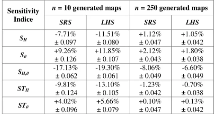
generated maps. The whole process is replicated 1000 times. Mean values with ± standard deviation bars for each estimate are shown on Fig 3. while Tab 2. gives for each estimate its standard deviation over the 1000 replicas, and the relative bias compared to its analytical value, for n = 10 and n = 250.
IV. RESULTS AND DISCUSSION
A. Exactness and precision of sensitivity indices estimates Fig 3. and Tab. 2 show that for small n, SH estimate has a
negative bias, while Sθ has a positive one. When n is low, the
small set of map simulations fails to capture the overall variability of Gaussian random field H: thus the influence of H variability on model output Y is underestimated; conversely the influence of θ is overestimated. This bias decreases when n increases.
LHS sampling of Gaussian random field H doesn’t bring improvement to estimates bias. For small n (n ≤ 10), LHS estimates have an additional bias which will be discussed in (IV.B). For larger sets of simulated maps (n ≥ 25), LHS procedure yields estimates whose relative biases are not significantly different from SRS estimates (significance tested with a Welch’s t-test for each value of n).
Figure 3. First order (top) and total order (bottom) sensitivity indices of input factors H (◦) and θ (+), depending on number n of generated maps and sampling strategy (SRS, LHS). Mean values with ±s.d interval over 1000 replicas. The dashed lines show the analytical results from Tab. 1.
TABLE II. EXACTNESS (RELATIVE BIAS IN %) AND PRECISION (±
STANDARD DEVIATION) OF SENSITIVITY INDICES ESTIMATES, FOR DIFFERENT SIZES n OF THE SET OF GENERATED MAPS
n = 10 generated maps n = 250 generated maps
Sensitivity Indice SRS LHS SRS LHS SH -7.71% ± 0.097 -11.51% ± 0.080 +1.12% ± 0.047 +1.05% ± 0.042 Sθ +9.26% ± 0.126 +11.85% ± 0.107 +2.12% ± 0.043 +1.80% ± 0.038 SH,θ -17.13% ± 0.062 -19.30% ± 0.061 -8.06% ± 0.049 -6.60% ± 0.049 STH -9.81% ± 0.124 -13.10% ± 0.105 -1.23% ± 0.042 -0.70% ± 0.038 STθ +4.02% ± 0.096 +5.66% ± 0.079 +0.10% ± 0.047 +0.13% ± 0.042
Tab. 2 also shows that LHS estimates have a slightly smaller standard deviation than SRS estimates: this gain is significant for many (Si, n) couples (Levene’s test). This
finding is consistent with more general results on variance reduction associated with LHS, in the case of sampling of scalar random variables (Helton and Davis, 2003).
B. Disturbance of spatial correlation by LHS
For small number n of generated maps (n = 3, 10), estimates computed with an LHS set of maps have an additional bias (underestimation of SH, overestimation of Sθ)
compared to SRS estimates. This additional bias can be explained by the fact that spatial correlation is disturbed by the LHS procedure. Fig 4. shows that maps from a LHS set have smaller spatial correlations than those from a SRS set, as discussed in (Pebesma and Heuvelink, 1999). But spatial correlation in map H influences the value of VM and thus the
values of sensitivity indices. (2) and (5) show that VM
decreases when spatial correlation in map H decreases (smaller range parameter a). This results in an additional underestimation of sensitivity indice SH when estimated with
a LHS set of maps. C. Discussion
LHS sampling of Gaussian random field H yields some improvement to the variability of sensitivity indices estimates but no significant improvement to estimates bias. These results can be explained by a general property of LHS: the more the target quantity (here the sensitivity indices) is additive in the variables sampled, the more LHS improves on SRS (Pebesma and Heuvelink, 1999). Here the values of sensitivity indices depend heavily on the variance VM of M,
the average water level over the study area ((5), (6) and (7)). But VM is not additive in sampled water levels hu: as a result,
the efficiency gain brought by LHS procedure is small.
TABLE III. EXACTNESS (RELATIVE BIAS IN %) OF THE ESTIMATES OF
EM(EXPECTATION OF M) AND VM, USING EITHER LHS OR SRS SIMULATION
STRATEGY, FOR DIFFERENT NUMBER n OF GENERATED MAPS
n = 10 n = 100 n = 200 Relative Bias SRS LHS SRS LHS SRS LHS
( )
EˆM ε -0.20a -0.014 -0.54 -2.10-3 -0.13 -4.10-5( )
VˆM ε -0.74 -0.28 -1.10 0.46 -0.59 -0.21a. Mean value of relative bias over 100 replicas
Figure 4. Average semivariograms for exponential model, SRS set of maps and LHS set of maps, n = 10 maps.
As an illustration, Tab 3. gives relative bias of estimates of expectation EM and variance VM, computed on SRS and LHS sets of maps. LHS brings a tremendous gain in estimate bias for the expectation EM (additive in sampled water levels hu), but no significant gain for the variance VM.
V. CONCLUSION
Sobol’ sensitivity indices were estimated on an artificial spatial model (derived from a complex model for flood risk economic assesment) with a 2D spatial input (a Gaussian random field), and compared to their analytical values. Two sampling strategies were used to generate realizations of input Gaussian random field: Simple Random Sampling and Latin Hypercube Sampling (higher CPU cost). Results show that (1) LHS sensitivity indices estimates have a significantly smaller variance (2) LHS sampling brings no significant improvement in estimates bias (3) for small sample size, disturbance of spatial correlation by LHS procedure yields an additional bias in estimates.
The poor improvement brought by LHS sampling comes from sensitivity indices not being additive in the variables sampled. Other ways should be sought to select input map realizations to perform sensitivity analysis of spatial models. These conclusions would be different if SA was computed “locally”, i.e. with a spatially distributed output (e.g. a map of damage). In this latter case, the spatial dimension of the problem would be reduced, and we could expect LHS to bring the same improvement as in a nonspatial context.
ACKNOWLEDGEMENTS
We thank Edzer J. Pebesma for giving us R code to perform LHS sampling of Gaussian random fields.
REFERENCES
Chilès, J. & Delfiner, P. (1999). Geostatistics: Modeling spatial uncertainty. New York: John Wiley.
Helton, J.C. & Davis, F.J. (2003). Latin hypercube sampling and the propagation of uncertainty in analyses of complex systems. Reliability Engineering & System Safety. 81 (1), 23–69.
Helton, J.C. & Davis, F.J. (2006). Sampling-based methods for uncertainty and sensitivity analysis. Multimedia Environmental Models. 32 (2), 135–154.
Lilburne, L. & Tarantola, S. (2009). Sensitivity analysis of spatial models. Int. Journal of Geographical Information Science. 23 (2), 151–168. Pebesma, E.J. & Heuvelink, G.B.M. (1999). Latin hypercube sampling of
gaussian random fields. Technometrics. 41 (4), 303–311.
Saltelli, A. et al. (2008). Global sensitivity analysis: The primer. Chichester: John Wiley.