Agricultural land pricing model for the Imperial Valley

AGRICULTURAL LAND PRICING MODEL

FOR THE IMPERIAL VALLEY

by

Mark Llewellyn Bixby B.S., Electrical Engineering

Duke University, 1988

Submitted to the Department of Urban Studies and Planning in Partial Fulfillment of the Requirements for the Degree of

Master of Science in Real Estate Development at the

Massachusetts Institute of Technology

September, 1994

@ 1994 Mark Llewellyn Bixby

All rights reserved

The author hereby grants to MIT permission to reproduce and to distribute paper and electronic copies of this thesis document in whole or in part.

Signature of Author

Mark L. Bixby Department of Urban Studies and Planning July 29, 1994 Certified by William C. Wheaton Professor of Economics Thesis Supervisor Accepted by William C. Wheaton Chairman Interdepartmental Degree Program in Real Estate Development

MASSACHUSETTS _INSTITUTE

AGRICULTURAL LAND PRICING MODEL

FOR THE IMPERIAL VALLEY

by

Mark Llewellyn Bixby

Submitted to the Department of Urban Studies and Planning in Partial Fulfillment of the Requirements for the Degree of

Master of Science in Real Estate Development

ABSTRACT

The Imperial Valley, located in the southeastern corner of California in Imperial County, is the tenth largest agricultural producing county in the United States. Over 489,000 acres of irrigated land produced nearly a billion dollars of revenue in 1993. The sale of agricultural properties in the Valley is of interest to property owners, farmers, developers, and investors.

This thesis analyzes ten years of agricultural property sales

transaction data. A database was built with information from 274 sales transaction records. A regression model was developed to describe the behavior of land price per acre. The benefits of regression analysis and its limitations are discussed for use in the sales comparison approach to appraisal. Local and national

economic trends are compared with the model predicted results.

Thesis Supervisor: Mr. William C. Wheaton Title: Professor of Economics

ACKNOWLEDGEMENTS

I would like to thank the following people:

Mr. Thomas K. Turner for his help collecting and copying hundreds of sales transaction reports, and for his patient responses to my

numerous phone calls and faxes.

Mr. Orlando B. Foote, a friend of my father, who gave me the names of the right people to interview to start my thesis research.

Mr. Tyler Lyon for the educational tour of the Valley and for his knowledge and appreciation of the land. Thanks also for the fresh produce I sampled and shared with my family.

Those other nice people listed in the Interview section of the Bibliography who took the time to answer my questions.

My wife Theresa for putting up with me and changing more than

her fair share of diapers while I punched in numbers and typed this thesis.

My three month-old son Ryan for just being, so that I was reminded

BIOGRAPHICAL NOTE

Mark plans to join the Bixby Land Company, a 100 year old property management and development company based in Long

Beach, California, in September 1994. The Company owns and operates commercial properties in the Long Beach area and agricultural properties in the Imperial Valley.

Prior to attending MIT for his Masters degree, Mark worked for

NGV Systems Inc., based in Long Beach, CA, from 1991 to 1993. He was a Sales Engineer for the NGV Technologies

Company division in 1992 and 1993 responsible for vehicle conversion sales and production scheduling. His other

responsibilities included writing conversion system documentation and taking the conversion systems through California Air

Resources Board certification.

In 1991 and 1992 Mark was the Northwestern Regional Sales Manager for CNG Cylinder Company, another division of NGV Systems. CNG Cylinder manufactures Compressed Natural Gas

(CNG) cylinders for the automotive industry. Mark was

responsible for sales calls, presentations, conferences, and shows in his territory. He was also responsible for factory technical support.

From 1990 to 1991 Mark worked as a Sales Engineer for Johnson Controls, Inc., Los Angeles, CA. His job entailed the layout, estimation, and sales of Heating, Ventilation, and Air Conditioning (HVAC) control systems for commercial and industrial buildings.

Mark received his Bachelor of Science in Electrical Engineering, from Duke University, Durham, NC in 1988.

In his free time the author likes bicycling, playing guitar, reading, skiing, surfing, traveling, and building things.

TABLE OF CONTENTS

Chapter Title

ONE Introduction

I Imperial Valley and Agriculture

Il Area Maps

Ill Why Build a Pricing Model?

IV Summary of Findings

TWO Appraisal of Agricultural Property

I Appraisal Factors

Il The Three Method Approach

IlIl Previous Use of Regression Analysis

THREE Data Collection and Methodology

I Tax Assessor Records

I1 Sales Transaction Comparisons

IlIl Explanation of Input Variables

IV Construction of Database

FOUR Development of Regression Models

I Hypothesis of Regression Models

I Types of Regression Models

IlIl Variables Created for Regression Models

IV Model Output

FIVE Agricultural Variable Analysis

I Soils

Il Crops

Ill Tiling / Drainage

IV Other Variables

SIX Locational Variable Analysis

I Proximity to Highways

I1 Proximity to Canals

III Proximity to Metro Areas

IV Zones

SEVEN Changes Over Time

I Time Dummy Variables

|I Local Agricultural Price Trends

IIl National Agricultural Price Trends

IV Sales Transactions

V Population Growth / Development

EIGHT Conclusions

I Regression Models in the Appraisal Process

LIST OF FIGURES

Figure Description

1-1 Locational Reference Map 1-2 Imperial Valley Map

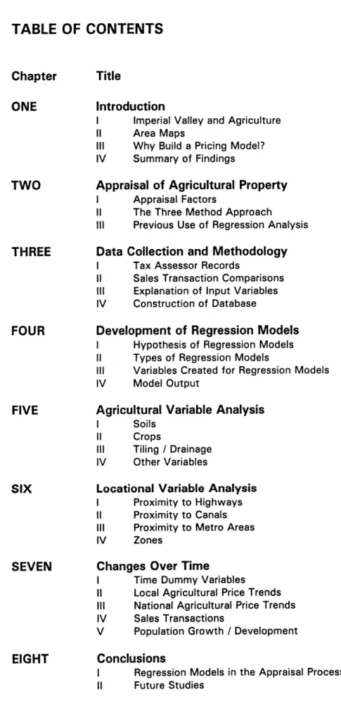
1-3 Imperial Irrigation District Index Map

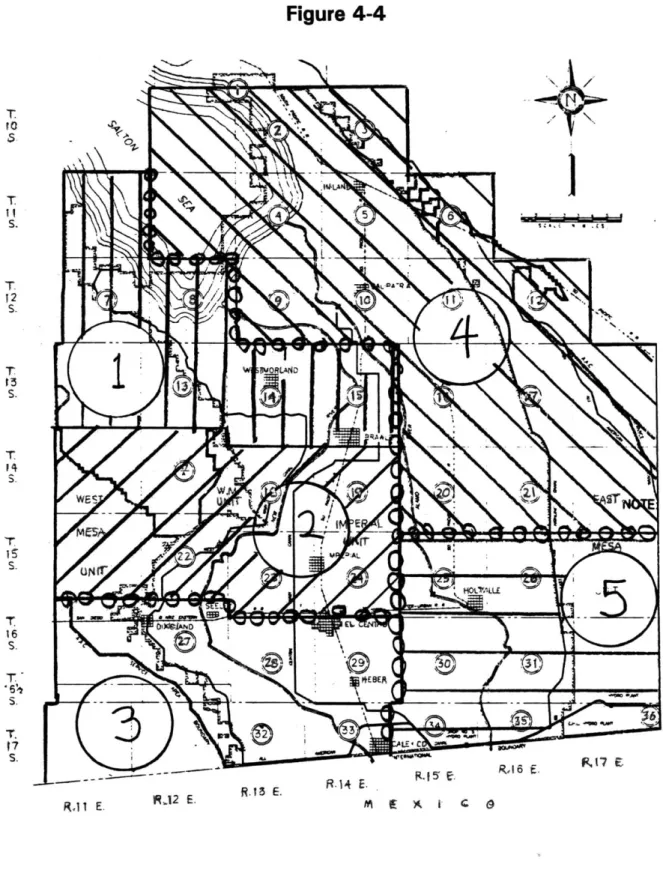
1-4 USDA Soil Conservation Service General Soil Map

2-1 Six Key Appraisal Factors

2-2 Histogram of Sales Transaction Data

3-1 Sales Transaction Data Summary

3-2 Soil Classifications

3-3 Metropolitan Area Codes

3-4 Examples of Database Variable Input 4-1 DURB Township and Range

4-2 DURB Township and Range Map 4-3 DZONE Township and Range

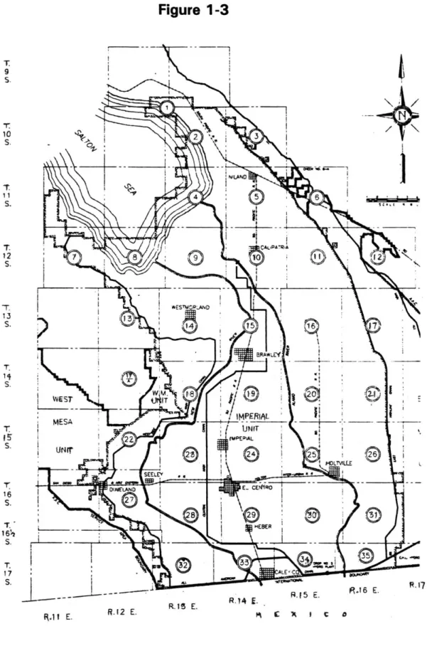
4-4 DZONE Township and Range Map

4-5 Examples of Regression Variable Input 4-6 Correlation Table

4-7 Regression Output Model 1 4-8 Regression Output Model 2

4-9 Final Regression Output Models 1 & 2 4-10 Model Predicted $/Acre Graph

5-1 Value of Agriculture Production from Imperial Valley

5-2 Agricultural Production Percentage Breakdown for 1992

5-3 Tiling Spacing Requirements 5-4 Tiling Cost Estimates

7-1 Local Agricultural Price Index Development

7-2 Local Agricultural Price Index Graph

7-3 Local Trend Comparison Graph Year to Year 7-4 Local Trend Comparison Graph Base Year 1983

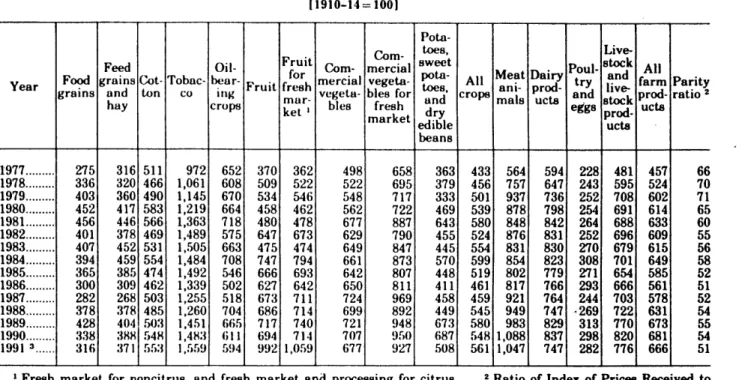
7-5 USDA Index Numbers: Prices Received by Farmers 7-6 National Trend Comparison Graph Year to Year

7-7 National Trend Comparison Graph Base Year 1983

7-8 Average Sales Transaction Size

7-9 Average Sales Transaction Price per Acre

7-10 Imperial Valley Population and Growth Statistics

7-11 Privately Owned Housing Unit Starts by City

CHAPTER ONE

Introduction

I Imperial Valley and Agriculture

Geographic

Imperial Valley is located in the South-eastern corner of California in Imperial County, bordering San Diego County to the West, Riverside County to the North, Arizona to the East, and Mexico to the South. San Diego is approximately two hours west by car on Interstate Highway 8, and Palm Springs is approximately two hours north by car. Figures 1-1 and 1-2 are included for reference.

Physiography

The Imperial Valley is a great basin sloping at an average of 0.1 percent from the Mexican border to the Salton Sea and covering approximately 990,000 acres (roughly 1550 square miles). Fossil remains indicate that the entire Valley floor was once several hundred feet below sea level and that the head waters of the Gulf of Mexico once extended as far north as the Chuckawalla Mountains (north of the Valley). Over time volcanic forces elevated the land and the Gulf

headwaters receded. The nearby Colorado River occasionally flooded and the runoff waters covered the Valley floor with soil and silt

93 8 Bakersfield 395 mn st Needl 9 93 resco nadSan Bernardino ₉ 95 9-. . . . . . . . . ... 101

... .... .... .. 9 5 Phoe...o Mesa

... M.. ...Temp

...Ila Bend

.. ... ...

Niland Chocolate Mountains OEast Mem West Mesa '1 c~. C CD -a ...

deposits rich in nutrients. Current Valley floor elevations range from

230 feet below sea level at the edge of the Salton Sea (1974) to 350

feet above sea level.

Climate

The Imperial Valley soils receive an average annual rainfall of approximately three inches. Without irrigation the soils have little

potential for productive farming. The average temperature in January is 54 degrees with a range of 29 to 80 degrees and the average

temperature in July is 92 with a range of 66 to 114 degrees.'

Development History

The Spanish began the first two missions in the Imperial Valley area near Yuma in 1776. They did not fortify the missions believing the Yuma Indians peaceful. In 1781 the Yuma felt their lands threatened

by a group of colonists headed for Los Angeles. All of the inhabitants

of the newly built missions were massacred. For many more years the Valley was more an obstacle to cross rather than a destination.

The first clues to the Valley's potential came from the Cahuilla Indians who farmed in the Valley:

1 _{Soil Survey of Imperial County, California, pg. 80.}

Since 1849 the fertility of most of this alluvial plain has been

recognized. Dr. Wozencraft then noted it. In an official report to the War Department in 1855 attention was called to the fact that the Cahuilla Indians were raising abundant crops of corn, barley and vegetables in the northwest part of the desert. The soil appeared to

be rich for wherever water touched it vegetation was abundant. 2

Southern Pacific completed a railroad line to Yuma, Arizona in 1877 and two years later the southern east-west railroad was completed. The line ran along the northeastern side of the Valley and Salton Sea

on its way to Los Angeles.

The persistence of a number of farsighted entrepreneurs led to the formation of the California Development Company (CDC) in April of

1896. Its mission was to convert the Colorado Desert (as the Imperial

Valley was known in the late 1 800's) into a productive agricultural region by diverting water from the Colorado River into an irrigation system distributing water throughout the Valley. Initially the CDC had difficulty raising money and convincing settlers to move to the area to farm the soil which was not yet irrigated.

Field work on the first canal began in December of 1900. Construction continued at a furious pace and by February 1902 the Valley had taken on a new character:

More than 400 miles of canals and laterals were built, more than

100,000 acres of land made ready for water, some 2000 eager 2 A History of Imperial Valley, pg. 22.

home seekers had been attracted, the towns of Imperial and Calexico started, and the bankrupt California Development Company turned into a concern worth millions. 3

By 1905 the CDC ran out of money. They were fighting creditors,

lawsuits, and an unruly river which repeatedly broke through dam and levee works. Southern Pacific Railroad, who was interested in the continued development of the Valley, loaned the company $200,000, enough for a controlling interest. By 1909 Southern Pacific chose to get out of the water business and the assets passed into receivership until 1911. The Imperial Irrigation District (ID) was formed to manage the water and properties.

The first canal cut in 1902 from the Alamo River on Mexican soil into the Valley began the long and interesting struggle over water rights from the Colorado River. After extended lobbying efforts on the part of

Valley government officials and others, Congress passed the Boulder Canyon Project Act (Swing-Johnson Bill) in 1929 providing for

construction of a dam in Boulder Canyon, a hydroelectric generation plant, and the All-American Canal. This guaranteed water rights to the Valley and would eliminate the flooding problems previously

experienced.

3 A History of Imperial Valley, pg. 48.

Imperial Irrigation District

The lID is a public utility providing water and power to Imperial County and parts of Riverside County. Today the IID operates the 82-mile-long All-American Canal, 148 miles of main canals, 1,442 miles of laterals, and has a "present perfected right" to 2.6 million acre-feet of Colorado River water. These canals and laterals irrigate approximately 489,000 acres of land, approximately half of all of the land in Imperial Valley. The district also provides power to over 80,000 users from its

hydroelectric, steam, gas, and diesel power plants.4

Current Demographics

As of January 1, 1992, the Imperial County population was

131,000 with 13,000 employed directly in agriculture. Industry

(including agri-business) employed 46,200. "Agriculture is still the largest industry in the county accounting for 28 percent of total wage and salary employment." 5 For populations of the cities see

Figure 7-10.

Current Agriculture Rankings

Imperial County is ranked as the 10th largest agricultural producing county in the United States. Over 489,000 irrigated acres produced

4 lID Fact Sheets.

5 Imperial County Annual Planning Information, pg. 10.

nearly a billion dollars of revenue in 1993. Figure 5-1 graphs the last 10 years worth of agricultural production by commodity type.

II Area Maps

Figure 1-1, the Locational Reference Map, shows the city of El Centro in relation to San Diego and Los Angeles. Figure 1-2 is a map of Imperial Valley showing the location of the ten cities (metro areas) referenced later in this thesis.

The Imperial Irrigation District Index Map (Figure 1-3) shows lID map index numbers, township and range numbers, main canals, and city grid outlines.

The USDA Soil Conservation Service General Soil Map (Figure 1-4) shows major soil group breakdowns and highlights the main

irrigated crop areas.

III Why Build a Pricing Model?

Price Variation

The sales transaction reports used in the regression analysis had a range in price per acre of agricultural land from $469 to $4,775. These variations were significant enough to warrant a quantitative

investigation of the characteristics affecting the price per acre. How much of the variation could a pricing model explain?

Agricultural Appraisal Process

In agricultural appraisal there are three approaches used to derive the value of a property similar to the three approaches in

commercial property appraisal. The appraiser determines a price for the property by reconciling the three approaches into a final value estimate. The appraisers interviewed for this thesis place much of the weight of their appraisals on the sales comparison approach.

Regression analysis is a worthwhile addition to the tools used in the comparison approach to appraisal. It is a statistical method used to explain the variation in a dependent variable (for example price per acre of real estate) caused by the change in one or more

independent variables (property size, locational characteristics, physical characteristics, etc.) With sufficient quality and quantity of data, regression analysis can be used to ground intuition with

statistical evidence computed from raw data. The coefficients calculated in the regression can be used in a model for predicting dependent variable values. Regression analysis is used extensively

in the physical, biological, economic, and social sciences to help distill useful information from reams of data.

The same database built for regression analysis can also be used to help pick the most appropriate property transactions for use in grid comparisons.

IV Summary of Findings

Two regression models were created to describe the variation in agricultural land price per acre. Both regression models had adjusted R2 numbers of approximately 50% indicating the models have

similar predictive abilities. These numbers are high enough to conclude that the model is useful in the property appraisal process.

Eleven variables were found to be statistically significant (not

including the time dummy variables). Both the level of tiling and the recorded crop types impacted the pricing model. The effect of urban influence was demonstrated as expected, meaning the model predicts that properties closer to urban areas have a higher sales price per acre than other similar outlying properties. However the area of urban influence was small and the majority of outlying sales transactions were unaffected by urban development patterns.

Locational analysis (unrelated to urban zones) demonstrated significant price differences between certain zones within the Valley. These differences can be partially explained by the distribution of soil types in an area, and may also reflect an

information effect where the buyer is aware of the quality of crops grown on surrounding properties.

The time dummy variables had the greatest single impact on the price per acre, affecting prices by as much as 33% in some years. It was difficult to link these price effects to local economic trends other than the impact of the whitefly infestation in 1991 and 1992. The model predicted prices seemed to follow the movements in

national agricultural indices but in a more radical fashion.

Figure 1-3

24

Figure 1-4

MEXICO

CHAPTER TWO

Appraisal of Agricultural Property

I Appraisal Factors

Three Agricultural Appraisers were interviewed for their thoughts on appraisal methodology, Mr. Jack Durrett, Mr. Andrew Erickson, and Mr. Thomas Turner. Mr. Durrett is an appraiser for Imperial County Assessor's office. Previously he worked for the Farm Credit

Services Southwest where he prepared a number of the Federal Land Bank of Sacramento Farm Sales Reports used as a data source for this thesis. Mr. Durrett described six key appraisal factors he used for property valuation:

FIGURE 2-1

Six Key Appraisal Factors

Factor Physical Description Valuation

Soils 100% Class 11 Excellent

100% Class Ill Average

< 50% Class IV* Fair

Size 40 - 60 acres Equal < 40 acres Lessor

> 160 acres Lessor

Shape Regular/Rectangular Average

Other Below Average

Location Proximity to Towns Higher - Closer

Access Highway Excellent

Paved Road Above Average

Dedicated Average

Not Gravel Below Average

Farmland Improvements Concrete Ditch Average

1/4 Mile Irrig. Runs Average Other Length Irrig. Runs Below Average

100' Tiling Spacing Average

* - Soil type # 114 is considered Class IV

Mr. Erickson listed soil types, farm improvements and location as the key factors in property valuation. He explained that location essentially determines soil types. Parts of the Valley are known for their soil qualities and the prices paid for particular properties reflect the knowledge of surrounding soil types. Mr. Erickson discussed tiling/drainage as the most important aspect of farm improvements, and mentioned ditch quality (concrete as average) and leveling as other important improvements. Mr. Erickson also discussed the shape of a property as a factor and pointed out problems with non-rectangular fields including: short row irrigation, more difficult tractor and land preparation work, more difficult crop dusting.

Mr. Turner emphasized soil type and tiling/drainage as the key factors in his property valuations. He listed other farmland

improvements, access roads to the property, shape, and location as other factors that have less influence on property prices.

11 The Three Method Approach

There are three methods for property valuation prescribed in The

Appraisal of Rural Property. Each method has its merits and pitfalls

but knowledgeable use of all three methods leads to an accurate property appraisal value. The methods are described below:

1. The value indicated by recent sales of comparable properties

in the market (the sales comparison method).

2. The value of a property's net earning power based on a capitalization of net income (the income capitalization method).

3. The current cost of producing a replica of the improvements,

less loss in value from depreciation, added to land value (the cost method).6

The valuations from each method of appraisal are then reconciled, a process by which the relative merit of each approach is considered and weighed in light of the information available on the piece of property.

Sales Comparison Method

The appraiser reviews comparable property sales to determine what price the sale property should bring on the open market. The

comparison approach for rural property concentrates on the land value which includes agriculture-related improvements to the land but not structures such as buildings, sheds, homes, or barns. Non-land improvements are simpler to appraise using the cost approach and these values can be added to the price of the property, however there

is no guarantee that a buyer is willing to pay what the seller has invested in non-agriculture related improvements.

6 The Appraisal of Rural Property, pg. 30.

Because each property has different physical characteristics the

appraiser must determine the key factors which affect the transaction price of the comparable properties and adjust the value of the

appraised property accordingly. It is important that the appraiser

ensure that the data obtained on comparable sales is accurate and that the comparable sales transactions were at arm's length (i.e. conducted under fair market conditions with no extraordinary conditions forcing the purchase or sale).

To determine the impact of variations between comparable property sales the appraiser must attempt to isolate the variation in a single characteristic for each characteristic which influences the sales price:

There are a number of acceptable methods for relating the sales to the subject property and for increasing or decreasing the price indication for the variations. Variations and adjustments between the comparable and the subject property may be related on a percentage basis, as a price per unit, or as a lump sum

adjustment.7

The common method for determining variations is to set up a series of data grids from which adjustment factors can be derived for variations in time of sale, soil variations, etc. This may be a difficult process when there are more influential property characteristics than there are comparable property sales. The appraiser's experience and knowledge of the area is most important when this is the case.

7_The

Appraisal of Rural Property, pg. 133.

According to the appraisers interviewed the sales comparison method is usually employed with three to five comparable property sales chosen. Mr. Turner described his method as searching his files for 10 to 12 property sales with similar characteristics then picking three to five comparable sales for use in a grid comparison.

Income Capitalization Method

The income capitalization method is used to analyze the future benefits of ownership of a property. The capitalization rate indicates the

relationship between the annual net earnings (or projected net earnings) from the property and the value or sales price:

1. Estimate the typical rental data, crop rotations, yields, and

average commodity prices for the area.

2. Estimate potential gross income for the property on either ownership or rental basis.

3. Estimate and deduct expenses of operation to derive net

operating income (net income before recapture).

4. Select an applicable capitalization method and technique.

5. Develop the appropriate rate or ratios.

6. Complete the necessary computations to derive an economic

value indication by the income capitalization approach.

Farm income streams are inherently unsteady from year to year. Mr. Turner explained that he uses a direct one year's rental rate

capitalization method (in the fourth step listed above) as recommended

8 The Appraisal of Rural Property, pg. 172.

by the American Society of Farm Managers and Rural Appraisers

(ASFMRA).

In 1992 local tenant farmers ran 64.8% of the total number of farms in the Imperial Valley with the remaining 35.2% owner operated.

Property rental rates ranged from $50 to $200 per net acre per year in the Valley. Agricultural property capitalization rates in 1992 in the United States ranged between three to six percent. Mr. Turner stated that capitalization rates in the Imperial Valley were usually in the range from four to five percent. Using the single year direct capitalization method these rates imply land prices per net acre of between $1,000 and $5,000.

The average waste acre percentage from the sales transaction data on the Imperial Valley is 9.1%. If we decrease the property value

estimates by 9.1% for the change from total acres to net acres the price range per total race shifts downward, from $910 to $4,550. Figure 2-2 is a histogram of total acre transaction prices from the data set for this thesis. This range of prices captures the majority of

HISTOGRAM OF SALES TRANSACTIONS

(10 YEARS COMPARISON DATA)

738 1007 1276 1545 1814 2084 2353 2622 2891 3160 3429 3698 3968 4237 4506

DOLLAR/ACRE SALES PRICE (WITHIN BIN)

20

z

-Cost Method

The cost method attempts to estimate the value of reproducing or replacing the improvements to the property while depreciating for the physical deterioration, functional obsolescence, and external

obsolescence. This method is less well suited to estimating a market value for agricultural properties because the value of the land and its productive potential is usually the main component of agricultural property value. The cost approach however is very useful for

establishing bounds on property prices and is commonly used in the appraisal process.

Ill Previous Use of Regression Analysis

A number of regression studies on the effects of property

characteristics on agricultural land values have been published. Palmquist and Danielson9 studied erosion and soil quality related effects on the price of agricultural land. They used two years of land transaction data on properties in North Carolina and concluded that soil quality had an effect causing these land values to differ by as much as 60%. They described their Hedonic regression equation as performing "quite well" and believed the results helpful:

The results can provide an estimate of the average increase in land value due to drainage. This information can be combined

9 A Hedonic Study of the Effects of Erosion Control and Drainage on Farmland

Values.

with drainage cost estimates in deciding whether or not to drain land.

In another study by King and Sinden10 data was gathered from five years of sales transactions of agricultural property in the Manilla Shire, New South Wales, Australia. Fifty transactions were selected for use in the study. The buyers, sellers, and agents were

interviewed for their knowledge of the factors affecting the transaction price. The authors developed four different models of price formation to test with the data. They found a number of interesting results including:

Buyers valued a given state of soil conservation and proximity to the nearest town more highly than the sellers... the positive influence of the geographic scope of search shows an information effect... Previous, unsuccessful attempts by the seller to sell had a negative influence on final price.

Canning and Leathers" constructed a regression model to describe the changes in land and building value due to changes in parameters (taxes and inflation) that change over time. Their study used USDA data series on land and building values.

10 _{Price Formation in Farm Land Markets.}

1 Inflation, Taxes, and the Value of Agricultural Assets.

CHAPTER THREE

Data Collection and Methodology

I Tax Assessor Records

The County Tax Assessor's office maintains a database with over 12,000 recorded property transactions for the last two years through March 1994. The records from prior years were available but not in a computerized format. The County database does not record the parcel size, a critical variable for a pricing model. Location, another important variable, is recorded in the County Tax Assessor's format which requires county tax assessor maps to locate properties. This

combination of factors ruled out a pricing model study using County Tax Assessor data.

I Comparisons From Ten Years of Sales Transactions

At the Farm Credit Services Southwest (FCSS) Mr. Turner

maintained a file containing comparison sales transaction reports dating back to 1967 that he and his predecessors had assembled.

For each year there were approximately 20 to 50 transactions records kept for use in property appraisal. Mr. Turner agreed to duplicate 10 years of reports for a quantitative study of comparable

sales transaction data. Figure 3-1, Sales Transaction Data Summary

graphs the number and year of the comparison sales transactions used in the database as well as the total acreage per year those transactions represent.

Mr. Turner explained that when an appraiser at FCSS learned of an agricultural property sale, he gathered the necessary information to complete a comparable sales transaction report. The appraiser collected this information from the County records, visits to the property/ies, USDA SCS Soil maps, and Imperial Irrigation District tiling maps. The data was verified with two sources, either the county, the buyer, the seller, or the real estate agent. Transaction data from 1984 to 1988 was recorded on Federal Land Bank of Sacramento Farm Sales Reports. From 1989 to 1992 the data was recorded on Western Farm Credit Bank Farm Sales Reports. Both reports are from the same organization but the report name was changed in 1988. In 1994 Mr. Turner began computerizing his reports for easier access and immediate use in his appraisals.

SALES TRANSACTION DATA SUMMARY 12,000 10,000 8,000 1984 1985 1986 1987 1988 1989 1990 1991 1992 1993 YEAR .mu ACRES 25

_z

Soil Name Storie Permea- Acres Acre % Index bility Soil # Class 1 105 117 Class I 100 101 106 107 108 109 110 118 119 120 137 142 143 144 Class IlIl 111 112 115 116 121 122 123 126 127 132 133 135 136 138 139 Class IV 103 114 124 125 128 130 131 Class V 113 134 58 mod 100 mod 85 77 37 52 50 30 59 60 90 76 90 57 100 60

Glenbar Clay loam Indio loam

Antho loamy fine sand Antho-Superstition complex Glenbar clay loam, wet Glanbar complex Holtville loam Holtville silty clay Holtville silty clay, wet Indio loam, wet Indio-Vint complex Laveen loam

Rositas silt loam, 0 - 2% slopes Vint loamy very fine sand, wet Vint fine sandy loam

Vint and Indio very fine sandy loams, wet Holtville-Imperial silty clay loams (sic) Imperial silty clay

Imperial-Glenbar sic, wet, 0 - 2% slopes Imperial-Glenbar sic, 2 - 5% slopes Meloland fine sand

Meloland very fine sandy loam, wet Meloland and Holtville loams, wet Niland fine sand

Niland loamy fine sand

Rositas fine sand, 0 - 2% slopes Rositas fine sand, 2 - 9% slopes Rositas fine sand, wet 0 - 2% slopes Rositas loamy fine sand, 0 - 2% slopes Rositas-Superstition loamy fine sands Superstition loamy fine sand Carsitas gravelly sand, 0 - 5% slopes Imperial silty clay, wet**

Niland gravelly sand Niland gravelly sand, wet Niland-Imperial complex Rositas sand, 0 - 2% slopes Rositas sand, 2 - 5% slopes Imperial silty clay, saline Rositas fine sand, 9 - 30% slopes Water Other 2,951 0.3 9,169 0.9 mod mod mod mod slow slow slow mod mod mod rapid slow rapid mod slow slow mod mod slow slow slow slow slow rapid rapid rapid rapid modslow modslow rapid slow slow slow slow rapid rapid slow 5,679 rapid 19,401 3,288 19,414 Totals 989,450 4,134 8,416 4,239 12,894 2,804 3,628 70,547 13,625 29,643 2,322 3,737 31,545 13,066 15,462 2,242 1,405 203,659 2,162 10,748 41,734 11,483 2,846 2,088 77,301 40,748 22,626 90,896 11,373 12,877 7,011 123,401 7,884 9,820 6,974 22,608 1,590 38 FIGURE 3-2 Soil Classifications 0.4 0.9 0.4 1.3 0.3 0.4 7.1 1.4 3.0 0.2 0.4 3.2 1.3 1.6 0.2 0.1 20.6 0.2 1.1 4.2 1.2 0.3 0.2 7.8 4.1 2.3 9.2 1.2 1.3 0.7 12.5 0.8 1.0 0.7 2.3 0.2 0.6 2.0 0.3 2.0 100.0

IlIl Explanation of Input Variables

Month and Year - The month (M) and year (YR) of each transaction were input.

Township and Range - The Township (TWNS) and Range (RNGE) of each transaction were recorded for use in sorting property sales by

location. Each individual Township and Range is approximately six miles by six miles.

Crops - Each sales transaction report provided information on the primary (CROP1) and secondary (CROP2) crops raised on the property. On some reports the crop type was spelled out and on most reports the crop type was numerically coded with the Federal Commodity

Codes (Fed Code 1 and 2). The crops listed most often included alfalfa

(181), sugar beets (132), cotton (121), and wheat (101/102). In the

years 1990 and later the sales transaction reports often recorded field crops (33) as primary crop with no secondary listing.

Soil Classification - In 1981 the United States Department of

Agriculture, Soil Conservation Service completed the most recent and thorough Soil Survey of Imperial County, California, written for use by farmers, ranchers, developers, builders, planners, and others. It

contains soil type descriptions, maps and tables, and is published in conjunction with a series of 37 detailed soil maps which break down the soils of the Valley into 44 separate soil types. These maps are used by the Soil Conservation Service when recommending the type, size, depth, and spacing of tiling lines for properties requiring drainage improvements. Appraisers also use the maps to determine the makeup of the soils when appraising properties.

The soil types are grouped into eight Capability Classes (I through VIII) which represent the suitability of soils for most kinds of field crops. In

Imperial Valley the first four classes of soils are of interest for cultivation:

Class I soils have few limitations that restrict their use.

Class Il soils have moderate limitations that reduce the choice of plants or that require special conservation practices, or both.

Class Ill soils have severe limitations that reduce the choice of plants, or that require special conservation practices, or both.

Class IV soils have very severe limitations that reduce the choice of plants, or that require very careful management or

both.12

The percentages of each soil type within a group were added to obtain the total percentage of a Capability Class. The variables CL1, CL2,

CL3, and CL4 were input.

12 Soil Survey of Imperial County, California, pg. 41.

Figure 3-2 is a reproduction of Table 3 reorganized by soil class numbers with the addition of Storie Index and permeability descriptions. The Storie Index rating is relative measure of the suitability of the soils for crop production within the Imperial Valley.

A rating of 100 is the most favorable rating, 0 the least favorable.

The permeability descriptions are associated with numbers (see Figure 5-3) which indicate the drainage rate in inches per hour.

Zoning - The variable ZONE recorded the property zoning. Some of the transaction sales reports indicated two types of zoning; the type of the largest portion was entered. A2 is the standard agricultural zoning code used in the Valley. A3 is the heavy agricultural zoning code which allows for uses such as feedlots, processing plants, and standard

agriculture.

Parcel Size - The variable SIZE recorded the total acre size of the property transaction.

Irrigated Acres - The variable ACRES recorded the size of the irrigated portion of the property which excludes houses, sheds, roads, canals,

Price - The variable PRICE$ recorded the total property transaction sales price including broker sales commission paid by the buyer. The variable BLDGS$ recorded the appraised value of the buildings and

improvements exclusive of agricultural improvements. The land value is the difference between the two variables.

Tiling Code - The variable TILE is a qualitative variable created by the author to code the perception of the level of tiling. The variable

was recorded as follows:

1. Tiled effectively; meets SCS recommendations, or spacing < 150'

2. Tiled but needs additional tiling to meet SCS recommendations, or tile spacing at > 150'

3. Not tiled, or less than 50 % tiled > 150'

Shape Code - The variable SHAP is another qualitative variable code created by the author to try to capture the importance of the

property layout discussed by the appraisers interviewed. The following guidelines were used:

1. Rectangular/regular

2. Irregular rectangular/triangular

3. Irregular/Obstacles (ditches, canals, railroad, etc.)

Access Code - ACXS is the third qualitative variable used to capture

the quality of the access to the property. The codes were assigned if the property had access provided by:

1. Paved Interstate/ State /County Highway (at least one side)

2. Paved road/good gravel (at least one side)

3. Unpaved, dirt only, or excessively long gravel road

Major Highways - Six major highways cross the Valley, state highways

86, 111, and the 115 are the major north-south state thoroughfares.

Interstate 8 runs east-west passing through El Centro between Yuma and San Diego. State highways 78 and 98 cross the Valley east-west.

The variable MHWY is the distance by car from an edge of the property to the nearest state highway or interstate highway. An

Imperial County road map was used and the distances have an

estimated accuracy of +/- 1/2 mile. It was expected that this variable would have a statistically significant effect on the property values because access to the property is important for leased machinery, maintenance, harvest, etc.

County Highways - County Highways 26, 27, 28, 29, 30, 31, 32, 33, and 80 comprise a grid work of access roads to a majority of the

Valley. The variable CHWY is the distance by car to the nearest county highway or state highway or interstate highway. As mentioned above

the accuracy is estimated at +/- 1/2 mile and the results were expected to be significant to the model.

Canals - The All-American Canal runs westward from the Colorado River to supply the Westside Main Canal, Central Main Canal, and the East Highline Canal which flow north through the Valley. The Imperial Irrigation District owns, maintains, and operates these canals and all water users pay water fees to the lID. These main canals feed a series of laterals which deliver water to each property. The lID also maintains the drainage ditch system which collects runoff and drainage water and delivers it to the Alamo or New Rivers. The Rivers flow into the

Salton Sea.

The variable CANAL measured the flow distance from the nearest main canal in miles to the property. The distances were estimated from an Imperial County road map and not traced along canal laterals. This variable was not expected to have much significance in a pricing model so the distances were estimated rather than laboriously traced along

plat book maps.

Metro Areas - The variable METR is a measure of the distance to the nearest metropolitan area from the list of ten areas below. The AREA

variable is a three character code for the metro area nearest the property listed below in Figure 3-3.

FIGURE 3-3

Metropolitan Area Codes

Westmoreland WES El Centro ELC

Niland NIL Seeley SEE

Calipatria CAL Holtville HOL

Brawley BRA Heber HEB

Imperial IMP Calexico CLX

IV Construction of Database

The database was constructed on a Microsoft Excel 5.0 Spreadsheet. The input data contains 274 rows of 23 columns totaling 6,302 data entries. Each transaction consisting of 23 entries was assigned a code number for reference to the appraiser's transaction sheet should there be questions about the data. Example database variable input data is shown in Figure 3-4. Additional variables which were created for use in the regression models are discussed in Chapter 4.

Figure 3-4

v- mNmin OvNc N WVm Mc N Na 0inow N M OOm e-N mm

N N N mm mNvNNN N i eT Vn

mO Z Olxzzaau 00- 2 0004mo o maa aaCma 00

x o g co o c x x - to m x x x m m m -n UN m m U L mm N NV NWN VT N OOOOOOOmOOOOOmqqqqOOOOOOOOO .NYNNN r'~N Nw r Nre o mm N N .N 0 )T 4W )W W ) 4C m Nm~ m W Orm N~ N OOO vv ,0N r OmNmmNNmmNNNeNcmNmmm.NmcreNONm a nn NmN N "W mc N M m vNY-v- Nnm NT- mN Ln PcnN Nm mmNNmNNmmmN Nm mmmeNe Ne vi W wt mwCR0r, wpqv co( c NinCm mwN mNNemmwemm mme NNmmCmbmNmmm Nm N m8 Cqom N a Vc m om Mo N- oFMT N m) N4 N- T 00000000 Na qqNinca o~m n oo T N N N N N m N 8888888 888 o mNNe 8 8 r -NN 8 rOW N

W@aNrowammemmNN a rNincmemin cam

ooo00oaaaaaaaa00990999990

ooOOOOOOOOOOOOOOOaaaOaa

8~a-oac a n !R~a'cc acaco mr, C4 co

iO N ~~co m r. r-.N- commc NN

m N- N N AN N v- m n m

aa- a aaou6 mn a 4 I.-~a a V

or N N m N N V N m in a

NN Nm NN NN N NNN NNN NNNNN

888 8888888888888888888888

5 ~ ~ m ~ mg ~~o 8 8 C82 ,S893

daad...oOdda* 6 ao da d vmvmowca-N m NcaWin 0 V n N T-WNc wrN ncacow m nm

N~ Vm LA rn coW incaov-cOrcocwi(a MmL

OOOOOOOO OOOOOOOOOOO.-OOOOOOOOOOOOO

in a d ;;8 i di c m coca d in; cia a ; V n 008ma coan~cam 00c fn to mt aa 0-mqio-n0 r 000* 0 0 Ir 000 aoo oa 00 a 66666 dc;c;

NNNNer-NNNN Ymee- NNNNNNNNrNYrNNNN rN mmmmNNmmmm NmN NNNmmmmmm mmm N am mmm Nm

N in M Va ca Ma VV N in inc m M V co vin coirWn -a inc W I in N1 in IV in V W)c W m w

m) in in v, V V v- v- m) vco ca W W VV N LM in Wo N i- m cai n cam coc Mo IDt(a N Va co

wa -aa w a V V V V qa -a -a V V - v a g anin

c0cow 0ooocc cow co0c 000 0C 0 0cDo w cw cOw cow Cowco wo co o co

~-~ -N N N4 N N N mm ml M V i n Wo N N N N, N Ow O W o 00 aT a1 a a

Nmmemm M~mmmm ureT-m It- v-

CHAPTER FOUR

Development of Regression Models

I Hypothesis of Regression Models

Multiple regression analysis tools are available in the more recent versions of Lotus 123 and Microsoft Excel, as well as in complete statistical software packages like SSPS (Statistical Package for the

Social Sciences) and STATA. Excel 5.0, the software used for most of the regression and analysis work in this thesis, is limited to analysis of 16 variables (including the dependent variable). For the final regression run which included 10 dummy year variables (for a total of 22 variables) SSPS Version 6.0 was used.

Multiple regression equations explain the variation in a dependent variable (for example price per acre of real estate) caused by the changes in the independent variables (property size, locational characteristics, physical characteristics, year of sale, etc.) The beta coefficients calculated in a regression run are used in a model for predicting dependent variable values if they are statistically significant.

To develop a model with the highest descriptive ability it is important to avoid multicollinearity. This means avoiding use of

highly correlated independent variables in the regression equation:

When multicollinearity is severe -- that is, when two or more of the independent variables are highly correlated with one another

-- we can run into difficulties interpreting the results of t tests

on the individual parameters.13

The correlation analysis tool in Excel 5.0 was used to create a correlation table (Figure 4-6) to review the statistical relations between variables. There were no significant correlations between variables by design so the model avoided multicollinearity problems.

I Types of Regression Models

Multiple regression model building is the process of adding,

deleting, and substituting variables and their types and formats into a multiple regression equation. The standard linear multivariate regression model is stated below where E(y) is the expected value

of the dependent variable,

p

E(y) =

So

pnxn

48 13 Intro to Statistics, pg. 529.

A second model type is the natural logarithmic-linear model which

has the following form:

E y) =

e

e

Taking the natural logarithm of both sides results in the following equivalent equation:

In [E(y)] =

$1

$nxn

The natural logarithm of the left hand side (original dependent variable) is taken creating a new variable which is entered as the dependent variable. Model 2 is entered into the regression software packages in the same manner as the linear model. The natural log-linear model described above is most appropriate in cases where the dependent variable y increases or decreases by a percentage

(factor), instead of by a fixed amount, as x increases.14

The software regression analysis tools calculate a number of

statistics for each regression "run" including four statistics for each variable which are referred to in this thesis; the beta coefficients, t statistics, and the adjusted multiple coefficient of determination (adjusted R 2). As more variables are added to a regression model

49 14 Intro to Statistics, _{pg. 557.}

the coefficient of determination (R 2) will increase even if the

variables added are not significant and do not contribute to the descriptive ability of the model. The adjusted R 2, a statistic which

adjusts for the number of variables in the model, is used.

Ill Variables Created for Regression Models

The standard variables entered in the regression are referred to as interval variables. Variables which take on values of only 1 or 0 are referred to as non-interval or dummy variables. In this thesis all dummy variables are prefaced with a D; for example DDEV standing for dummy development variable.

$PERACRE - This variable is the difference between PRICE$ and BLDG$ divided by SIZE.

L$PRACRE - This is the natural log of the variable $PERACRE.

SIZEACRE - Simply the size of the property in acres.

WST% - This variable is the waste acres (SIZE less ACRE) divided

by SIZE. The average value of this variable is 9.1%.

DCL2, DCL3, DCL4 - These are equal to 1 if the value in their

respective Capability Class CL2, CL3, and CL4 is greater than 0.75.

DTILE - This is equal to 1 if TILE is equal to 1.

DCROP - This is equal to 0 when the primary crop CROP1 is 181

(Alfalfa) and the secondary crop CROP2 (Sugar Beets) is 132 or if CROP1 is equal to 33 (Field Crops). These common numbers appear to have been the default crop description used by the appraisers. DCROP is equal to 1 for any crops other than the default crops.

DDEV - This is a locational variable equal to 1 if METR is less than 3 (miles) and the metro area variable AREA is equal to BRA, IMP, or ELC.

DDEV2 - This is another locational dummy variable which is equal

to 1 if METR is less than 2 (miles) and the metro area variable AREA is equal to BRA, IMP, ELC, HOL, CLX, or CAL.

DURB - This is a third locational dummy variable which is equal to 1

if the Township and Range (TWNS, RNGE) variables equal any of the following pairs:

FIGURE 4-1

DURB Township and Range

T R T R T R T R

12 14 14 14 15 15 17 14

13 13 15 13 16 13 17 15 13 14 15 14 16 14

These Township and Range pairs cover those areas designated in the Imperial County General plan for development which include the

metro areas of Brawley (BRA), Imperial (IMP), El Centro (ELC), Holtville (HOL), Calexico (CLX), and Calipatria (CAL).

FIGURE 4-3

DZONE Township and Range

ZONE 1 ZONE 2 ZONE 3 ZONE 4 ZONE 4 ZONE 5

T R T R T R T R T R T R 11 11 14 11 16 11 12 15 15 15 12 11 14 12 16 12 10 12 12 16 15 16 12 12 14 13 16 13 10 13 13 15 15 17 13 11 14 14 16 14 10 14 13 16 16 15 13 12 15 11 17 11 13 17 16 16 13 13 15 12 17 12 11 12 14 15 16 17 13 14 15 13 17 13 11 13 14 16 17 15 15 14 17 14 11 14 14 17 17 16 11 15 17 17 12 13 12 14

DZ1, DZ2, DZ3, DZ4, DZ5 - These are dummy variables created

from the TWNS and RNGE variables. The variables are equal to 1 if the Township and Range pairs fall within the respective zone

categories listed in the Figure 4-3 below. Figure 4-4 highlights the zones.

Figure 4-2

Figure 4-4

54

D84,D85,D85,D87,D88,D89,D90,D91,D92,D93-These are equal to 1 if YR equals 84 for D84, YR equals 85 for

D85, etc.

DCH - This dummy variable is equal to 1 if the variable CHWY is

equal to 0 (in other words equal to 1 if the property is located adjacent to a County highway) and equal to zero otherwise.

DMH - This dummy variable is equal to 1 if the variable MHWY is equal to 0 (in other words equal to 1 if the property is located adjacent to a state or interstate highway) and equal to zero otherwise.

DZONE - This dummy variable is equal to 1 of the zoning code was

equal to A3, heavy agriculture.

Figure 4-5 is an Excel spreadsheet with sample regression input variables.

REGRESSION VARIABLE INPUT

MODEL I MODEL2 INDEP VAR.= = >

$PERACRE L$PRACRE SIZEACRE WST% CHWY

2,872 2,813 2,200 1,977 3,000 3,250 3,488 3,441 2,500 3,465 3,100 3,935 3,383 610 3,600 3,109 3,296 2,200 3,231 2,182 2,700 3,000 3,666 2,467 2,800 3,525 2,759 3,249 2,949 3,333 3,250 3,330 2,482 3,720 7.9629 7.9418 7.6962 7.5892 8.0064 8.0864 8.1571 8.1434 7.8240 8.1505 8.0392 8.2775 8.1264 6.4135 8.1887 8.0422 8.1004 7.6962 8.0806 7.6879 7.9009 8.0064 8.2069 7.8106 7.9374 8.1675 7.9225 8.0860 7.9891 8.1117 8.0864 8.1108 7.8168 8.2213 SOIL TYPES 56.4 0.04 0.50 800.0 0.10 0.50 180.0 0.09 -86.0 0.14 2.50 80.0 0.06 -119.0 0.05 0.50 80.0 0.04 3.50 79.0 0.05 3.00 40.0 0.08 2.00 125.5 0.04 3.50 160.0 0.06 2.00 420.0 0.07 -81.0 0.06 0.50 200.0 0.05 2.00 240.0 0.05 -320.0 0.25 1.00 98.0 0.10 1.00 80.0 0.08 0.50 160.0 0.06 -275.0 0.16 6.00 80.0 0.05 4.00 80.0 0.08 1.50 783.0 0.04 -15.0 0.27 0.50 80.0 0.05 -163.0 0.02 -145.0 0.06 1.00 112.9 0.04 1.00 39.0 0.15 1.00 390.0 0.06 0.50 160.0 0.11 -560.0 0.08 -1,073.0 0.05 -82.0 0.09 1.50 DCL2 0 0 0 0 0 0 0 0 1 0 1 0 0 0 0 1 0 0 0 0 0 0 0 0 0 0 0 1 0 0 0 0 0 0 DCL3 0 0 0 0 0 1 0 0 0 1 0 0 0 0 0 0 0 1 0 0 1 0 1 0 1 0 0 0 0 1 0 0 0 0 DCL4 0 0 0 0 0 0 0 0 0 0 0 0 0 0 0 0 0 0 0 0 0 1 0 0 0 0 0 0 0 0 0 0 0 0 ZONES YEARS

DTILE DCROP DDEV DZ2 DZ3 DZ4 DZ5 D85 D86 D87 D88 D89 D90 D91 D92 D93

0 0 0 0 0 0 0 0 0 0 0 0 0 0 0 0 0 0 0 0 0 0 1 0 0 0 0 0 0 0 0 0 1 0 0 1 0 0 0 0 0 0 0 0 0 0 0 0 1 1 0 0 0 1 0 0 0 0 0 0 0 0 0 0 0 1 0 0 0 1 0 0 0 0 0 0 0 0 0 0 0 1 0 1 0 0 0 0 0 0 0 0 0 0 0 0 0 1 0 0 0 1 0 0 0 0 0 0 0 0 0 0 1 1 0 0 0 1 0 0 0 0 0 0 0 0 0 0 1 1 0 0 0 0 0 0 0 0 0 0 0 0 0 0 1 1 0 0 0 1 0 0 0 0 0 0 0 0 0 0 0 1 0 0 0 0 1 0 0 0 0 0 0 0 0 0 1 1 0 0 0 0 1 0 0 0 0 0 0 0 0 0 1 1 0 0 1 0 0 0 0 0 0 0 0 0 0 0 0 1 0 1 0 0 0 0 0 0 0 0 0 0 0 0 0 1 0 1 0 0 0 0 0 0 0 0 0 0 0 0 0 1 0 0 0 0 0 0 0 0 0 0 0 0 0 0 0 0 0 0 0 0 1 0 0 0 0 0 0 0 0 0 0 0 0 0 0 0 1 0 0 0 0 0 0 0 0 0 0 0 0 0 0 0 1 0 0 0 0 0 0 0 0 0 0 0 0 0 0 1 0 0 0 0 0 0 0 0 0 0 1 1 0 0 0 1 0 0 0 0 0 0 0 0 0 0 0 0 0 0 0 1 0 0 0 0 0 0 0 0 0 0 0 0 0 0 0 0 1 0 0 0 0 0 0 0 0 0 0 0 0 1 0 0 0 0 0 0 0 0 0 0 0 0 0 1 0 0 0 0 1 0 0 0 0 0 0 0 0 0 0 0 0 0 1 0 0 0 0 0 0 0 0 0 0 0 0 1 0 0 0 1 0 0 0 0 0 0 0 0 0 0 1 1 0 0 1 0 0 0 0 0 0 0 0 0 0 0 1 0 0 0 0 0 1 0 0 0 0 0 0 0 0 0 0 0 1 0 1 0 0 0 0 0 0 0 0 0 0 0 1 0 0 0 0 1 0 0 0 0 0 0 0 0 0 0 0 0 0 0 0 0 1 0 0 0 0 0 0 0 0 0 0 1 1 1 0 0 0 1 0 0 0 0 0 0 0 0 1 0 1 0 1 0 0 1 0 0 0 0 0 0 0 0 -41 CD ,3