Aggregation bias, information loss, and trade-coefficient stability in the multiregional input-output model

MULTIREGIONAL INPUT-OUTPUT MODEL by

WILLIAM H. CROWN

B.A., University of Vermont (1976)

M.A., Boston University (1979)

Copyright by William H. Crown

0

SUBMITTED IN PARTIAL FULFILLMENT OF THE REQUIREMENTS FOR THE

DEGREE OF DOCTOR OF PHILOSOPHY

at the

MASSACHUSETTS INSTITUTE OF TECHNOLOGY (January 1982)

The author hereby grants to M.I.T. permission to reproduce and

to distribute copies of this thesis document in whole or in part.

Signature of the Author

Department of Urban Studies and Planning, January 1982

Certified b

Accepted by

Thesis Supervisor

Ch'airfn, Departmental Committee

Rotch

SEP 21 1582

by

William H. Crown

Submitted to the Department of Urban Studies and Planning in Partial Fulfillment of

the Requirements for the Degree of Doctor of Philosophy

ABSTRACT

The impacts of aggregation on estimation bias and questions. concerning the stability of technical coefficients in single-region input-output models received a great deal of attention in the literature

throughout the 1950s and 1960s. The comparatively recent development of several multiregional models requires that concerns about the problems related to aggregation be reconsidered from a multiregional perspective.

Furthermore, because of the spatial characteristics of multiregional models, the importance of interregional trade for accurate output

estimates and the issue of trade-coefficient stability also need to be given more attention.

In this thesis, a theoretical framework is developed to analyze the importance of trade, aggregation bias, and information loss that builds upon research conducted by previous analysts. In the case of aggregation bias and information loss, this theoretical work represents an extension from single-region analyses to multiple regions. This extension requires explicit treatment of interregional trade. The theoretical work concerning the importance of trade for accurate output estimates deals with clarifying the issue of when it is necessary to include detailed state-to-state trade data in the multiregional input-output (MRIO) model. It is shown that by correctly adjusting regional final demands by the amount of net-trade balances, accurate output estimates can be obtained without detailed interregional trade data. This is true, however, only when accurate regional production and

consumption data are available with which to obtain the net-trade balance estimates. Furthermore, interregional trade data are necessary for

several other reasons: (1) for ensuring the accuracy of detailed

multipliers; (2) for their usefulness in balancing the MRIO accounts; and (3) for conducting transportation studies.

An analysis of the effects of aggregation on estimation bias in the MRIO model is also conducted. This analysis indicates that

aggregation of the base-year accounts results in very little estimation bias. However, introducing a different final demand structure can result in substantially different conclusions concerning the size of the

aggregation bias.

The fact that aggregation may lead to loss of information content

This suggests that regional analysts, who often use input-output models for purposes other than impact analysis, need to be very careful about the aggregation of data. This is particularly true in multiregional input-output models, where the quantity of data often requires

aggregation to allow meaningful interpretation of the results. Finally, if interregional trade data are to be used in a multiregional model, it is also necessary to be concerned about the

stability of trade patterns over time. Including obsolete trade data in a model may introduce considerable error into the estimates obtained. To shed some light on this topic, an analysis of trade coefficient stability

is carried out using 1967 and 1972 Census of Transportation data with

detail for three transportation modes and twenty commodity

classifications on a state-to-state basis. The results show that the stability of the trade data decreases with disaggregation. Whether or

not interregional trade data are sufficiently stable for use by regional analysts is a topic requiring further study, however. It seems likely

that the data may be stable enough for some types of studies but not for

others.

Thesis Supervisor: Karen R. Polenske

Title: Professor

Any research effort such as that represented by this thesis owes a debt of gratitude to many people. The contributions of these individuals range from the provision of data and intellectual insights to the equally important provision of moral support and encouragement. A complete

enumeration is impossible; to those omitted, my debt is no less great. Nevertheless, some individuals deserve special mention.

Above all, I would like to express my appreciation to Professor Karen R. Polenske -- thesis supervisor, academic advisor, and friend. Early discussions with Karen focussed the direction of the work. Her subsequent enthusiasm and guidance throughout the course of the research kept it on track. In addition, Karen's generous provision of computer resources and willingness to provide rapid comments on drafts at every stage were crucial to the progress and eventual completion of the thesis.

Similarly, thanks go to Professors Robert Dorfman of Harvard and Alan Strout of the Massachusetts Institute of Technology, for providing thoughtful comments on all of the chapters. Their suggestions

significantly affected both the direction and the quality of the research.

I would also like to thank Priscilla Kelly for her efforts in typing the equations, as well as many of the tables in the thesis. Her ability to decipher my handwriting was remarkable and her professionalism

commendable.

Financial support and data were provided by several sources. The research on trade-coefficient stability was funded by Jack Faucett

Associates, Inc. Jack Faucett Associates also provided the Census of Transportation computer tapes used for the trade coefficient analysis. Professor Karen R. Polenske provided access to the multiregional

input-output (MRIO) model and database that was used for the analysis of aggregation bias, information loss, and the impacts of interregional trade on the output estimates. Funding for some of the later stages of the research was provided by a subcontract with Boston College in

conjunction with their efforts to build the multiregional policy impact simulation (MRPIS) model for the Department of Health and Human Services.

Finally, I would like to express my appreciation to my parents for their support of my education and to my wife Robin, who encouraged and supported my efforts in ways too numerous to list. The sacrifices made by Robin were unquestionably the largest factor in enabling me to

complete the thesis. Those sacrifices will never be forgotten, nor probably ever repaid.

Page

ABSTRACT ii

ACKNOWLEDGMENTS iv

TABLE OF CONTENTS vi

LIST OF TABLES viii

LIST OF FIGURES x

CHAPTER 1

TRADE RELATIONSHIPS IN MULTIREGIONAL MODELS 1

CHAPTER 2

A METHODOLOGY FOR ANALYZING THE ROLE OF TRADE IN THE

MRIO MODEL 6

TOTAL INTERREGIONAL TRADE EFFECTS 9

MRIO Accounts and Model 9

Interregional Trade Effects in the MRIO model 15

AGGREGATION BIAS AND INFORMATION LOSS IN THE MRIO MODEL 20

Aggregation Bias in the MRIO Model 21

Aggregation and Information Loss 31

Underlying Principles of Information Theory 34

Quantifying Information Loss in the MRIO Model 38

INTERTEMPORAL TRADE-COEFFICIENT STABILITY 41

Definition of Trade-Coefficient Stability 43 Effects of Trade-Coefficient Instability 47

CONCLUSIONS 48

CHAPTER 3

EMPIRICAL EVIDENCE REGARDING THE ROLE OF TRADE IN THE

MRIO MODEL 50

INTERREGIONAL TRADE EFFECTS 51

AGGREGATION BIAS AND INFORMATION LOSS 57

Chapter 3 (continu'ed)

TRADE-COEFFICIENT STABILITY 69

Consistency Between 1967 and 1972

Industry Definitions 71

Aggregate Intermodel Substitution 72

Analysis of Trade-Coefficient Stability 76

CONCLUSIONS 89

CHAPTER 4

CONCLUSIONS AND DIRECTIONS FOR FUTURE RESEARCH 93

INTERREGIONAL TRADE EFFECTS 93

AGGREGATION BIAS AND INFORMATION LOSS 96

TRADE-COEFFICIENT STABILITY 99

DIRECTIONS FOR FUTURE RESEARCH 100

APPENDIX A: MATRIX STRUCTURE OF THE MRIO MODEL 103

The MRIO Accounting Framework 104

The MRIO Accounts and Model 109

Matrix Structure of the MRIO Model 112 APPENDIX B: MATHEMATICAL FORMULATION OF INTERREGIONAL

FEEDBACK EFFECTS 117

Feedback Effects in an Interregional

Input-Output Model 118

Feedback Effects in the Multiregional

Input-Output Model 121

APPENDIX C: MRIO CLASSIFICATION SCHEMES 124

APPENDIX D: ADDITIONAL RESULTS RELATED TO

INTERREGIONAL TRADE EFFECTS 128

APPENDIX E: TRANSPORTATION COMMODITY CLASSIFICATION CODES 131 APPENDIX F: ADDITIONAL RESULTS RELATED TO TRADE-COEFFICIENT

STABILITY 137

BIBLIOGRAPHY 174

Table Title Page

3.1 PERCENTAGE DIFFERENCE BETWEEN BASE CASE AND 1963 REGIONAL OUTPUTS RESULTING FROM OMISSION

OF INTERREGIONAL TRADE 53

3.2 PERCENTAGE DIFFERENCE BETWEEN BASE CASE AND 1963 REGIONAL OUTPUTS RESULTING FROM OMISSION

OF INTERREGIONAL TRADE (WITH~NET-TRADE

BALANCE ADJUSTMENT) 55

3.3 AGGREGATION BIAS: 1963 ESTIMATED OUTPUTS,

19-INDUSTRY, 9-REGION CASE 58

3.4 AGGREGATION BIAS: 1963 ESTIMATED OUTPUTS,

79-INDUSTRY, 51-REGION CASE 61

3.5 AGGREGATION BIAS: 1980 ESTIMATED OUTPUTS,

19-INDUSTRY, 9-REGION CASE 63

3.6 AGGREGATION BIAS: 1980 ESTIMATED OUTPUTS,

79-INDUSTRY, 51-REGION CASE 64

3.7 INFORMATION LOSS DUE TO AGGREGATION 67

3.8 PERCENT DISTRIBUTION OF COMMODITIES SHIPPED

IN THE UNITED STATES BY TRANSPORTATION MODE 73 3.9 MEANS, STANDARD DEVIATIONS, AND COEFFICIENTS

OF VARIATION FOR TRADE-COEFFICIENT CHANGES,

1967-1972 79

3.10 MEANS, STANDARD DEVIATIONS, ZERO ENTRIES, AND COEFFICIENTS OF VARIATION FOR

TRADE-COEFFICIENT CHANGES: NONZERO ENTRIES,

1967-1972 81

3.11 DISTRIBUTION OF RAIL TRADE-COEFFICIENT CHANGES 83 3.12 DISTRIBUTION OF TRUCK TRADE-COEFFICIENT CHANGES 84 3.13 DISTRIBUTION OF OTHER TRADE-COEFFICIENT CHANGES 85 3.14 DISTRIBUTION OF PERCENTAGE TRADE-COEFFICIENT

CHANGES FOR RAIL 86

3.15 DISTRIBUTION OF PERCENTAGE TRADE-COEFFICIENT

CHANGES FOR TRUCK 87

3.16 DISTRIBUTION OF PERCENTAGE TRADE-COEFFICIENT

CHANGES FOR OTHER 88

C.1 MULTIREGIONAL INPUT-OUTPUT CLASSIFICATION

FOR NINETEEN INDUSTRIES 125

C.2 INDUSTRIAL CLASSIFICATION SCHEME

(79 to 3 Industries) 126

C.3 REGIONAL CLASSIFICATION SCHEME

(51, 9, and 3 Regions) 127

D.1 PERCENTAGE DIFFERENCE BETWEEN BASE CASE AND 1963 REGIONAL OUTPUTS RESULTING FROM

OMISSION OF INTERREGIONAL TRADE FOR SERVICE INDUSTRIES (WITH NET-TRADE BALANCE

ADJUSTMENT) 129

D.2 1963 CALCULATED BASE CASE OUTPUTS,

19 INDUSTRIES, 9 REGIONS 130

F.1 AGGREGATE TRADE COEFFICIENT DIFFERENCES

1967 to 1972 ₁₃₈

F.2 PERCENTAGE CHANGES IN AGGREGATE TRADE

COEFFICIENTS, 1967-1972 150

F.3 AGGREGATE 1967 TRADE COEFFICIENTS 162

Title

RELATIONSHIP OF PROBABILITY SIZE TO INFORMATION CONTRIBUTION

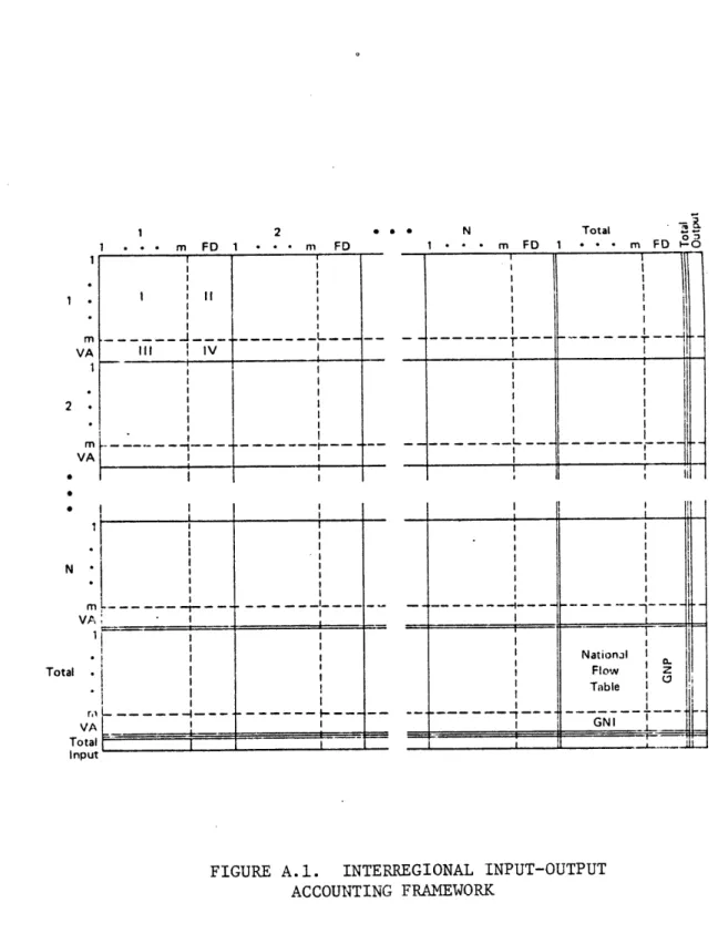
IRIO ACCOUNTING FRAMEWORK

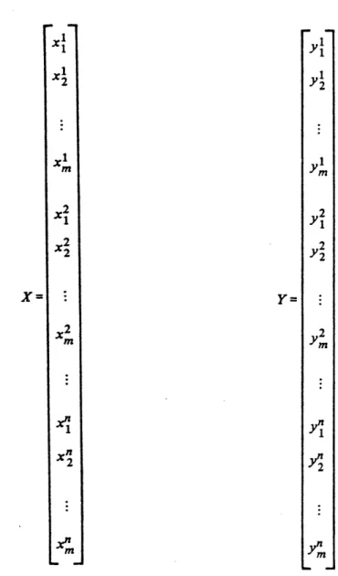
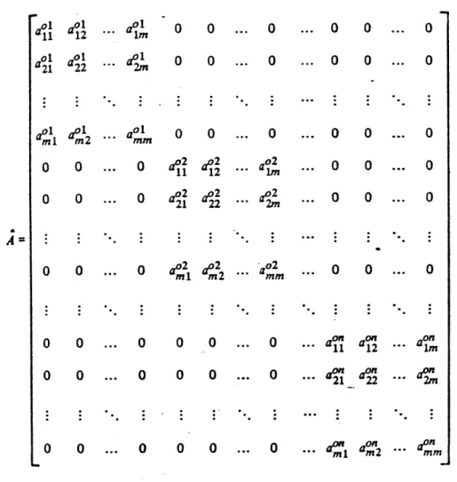
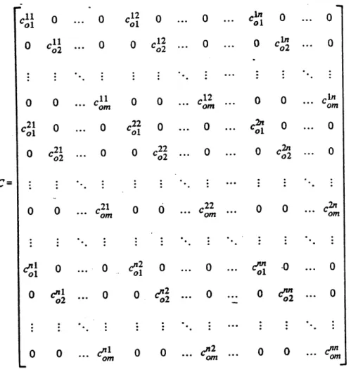
MRIO OUTPUT AND FINAL DEMAND VECTORS EXPANDED TECHNICAL COEFFICIENT MATRIX EXPANDED TRADE COEFFICIENT MATRIX

DETAILED MATRIX BALANCE EQUATIONS (REARRANGED)

x Figure 2.1 A.1 A.2 A.3 A.4 A.5 Page 36 105 113 114 115 116

CHAPTER 1

TRADE RELATIONSHIPS IN MULTIREGIONAL MODELS

Economics is sometimes defined as the study of the allocation of scarce resources among competing ends. When a spatial dimension is added to this.statement, it becomes a definition of regional economics.

Because trade is inevitably the process by which resources are allocated, the study of trade would seem to be of particular interest to regional analysts. In actuality, the amount of interregional trade research that

has been done is quite limited. Part of the reason for this lack of research stems from the amount of work that has been done in the field of international trade. In fact, most of the theoretical work that has been done on interregional trade has borrowed its conceptual framework

directly from the international literature. There is, however, another

reason for the lack of interregional trade research--paucity of data. Only recently, with data for several years available from the U.S. Census of Transportation, have regional analysts been provided with a

significant database of interregional trade information. Even this

information has severe drawbacks, however, some of which are noted in

Chapter 3.

Partly because of the difficulty in assembling interregional trade data, several issues related to the role of trade in multiregional and interregional input-output models have not been adequately resolved. Among the most important of these issues are the significance of

interregional trade data for accurate industrial output estimates, the impact of aggregation on estimation bias and information loss, and trade-coefficient stability. In this thesis, these three issues are

studied with an explicit recognition of their interrelated nature.

Although by dealing with all three, it was difficult to study any one of

the issues in great detail, this approach was considered to be necessary because of the complex interrelationships among the three areas. These interrelationships have not been clearly delineated in the literature.

As a result, the literature related to the importance of interregional trade data in multiregional and interregional input-output models and trade-coefficient stability has been largely inconclusive.(1) In fact, only the literature with respect to aggregation bias in single-region input-output models appears to have been very definitive.

The issue of aggregation in single-region input-output tables was of great interest to analysts in the late 1950s and early 1960s, but was found by these analysts to have negligible impacts on estimated outputs. Recently, Miller and Blair (1980, 1981) have conducted studies to

determine whether aggregation is a serious problem in interregional and multiregional input-output models. The authors presented results,

however, only for total regional outputs. Because it would be expected that the output for each industry in a region would be more sensitive to aggregation bias than total regional outputs, additional work needs to be done before the empirical significance of the aggregation problem can be resolved.

Of course, regional analysts employ interregional and

multiregional input-output models for purposes other than conducting impact analyses. A major attribute of these models is the detail that

they provide in terms of interregional, interindustry transactions. In

(1) For a brief review of the literature, see Richardson (1972, pp.

the late 1960s several analysts recognized that, in addition to estimation bias, aggregation may result in a loss of information in input-output models. To measure the loss of information from

aggregation, quantitative methods were developed using concepts from information theory. The extent of this research has been very limited, however, and no studies have been conducted to assess the impacts of aggregation on a multiregional input-output system.

Although the literature has focused primarily on aggregation bias and technical coefficient stability in single-region models, the recent growth in multiregional modeling requires that the topics of aggregation bias and information loss be reconsidered from a multiregional

perspective. Because of the difficulty of collecting interregional trade data, several studies have been conducted concerning the size of

interregional trade effects in interregional and multiregional models. These studies have sought to determine whether interregional trade data are necessary for making accurate estimates of regional industrial

outputs with multiregional or interregional input-output models. A similar type of study is carried out in this thesis. However, the

research presented in this dissertation differs from previous studies for reasons that are discussed in Chapter 2.

The final topic dealt with in the thesis, is an investigation of the stability of interregional trade patterns. Such a study is important for both empirical and theoretical reasons. The empirical reasons

include errors introduced into multiplier and output calculations with multiregional and interregional input-output models, as well as the

implications for how often interregional trade data must be assembled. A study of trade stability is important for theoretical reasons because

there is no a priori reason to expect interregional trade patterns to be

either stable or unstable over time (Richardson, 1972, pp. 76-82). This

is an issue that can only be resolved by a comprehensive analysis of

trade-coefficient stability. The research presented in this dissertation is a first step towards understanding changes in trade patterns over time.

The current assembly of the 1977 MRIO accounts provides an

illustration of the need for a study combining an analysis of the importance of interregional trade in the MRIO model with a study of

trade-coefficient stability and the impacts of aggregation on estimation bias and information loss. The 1977 MRIO accounts are being assembled to

form the business component of the Multiregional Policy Impact Simulation

(MRPIS) model.(1) The issues dealt with in this thesis are important to

the MRPIS research for a number of reasons: (a) the MRPIS model is being designed to investigate the impact of different federal programs on

income distribution, and interregional trade is the mechanism by which

these impacts are distributed to the different sectors in each region;

(b) for various reasons related to data availability and model development, certain segments of the MRPIS model must be run at an

aggregate level. This will have implications for aggregation bias and

information loss in the model; and (c) the stability of the trade coefficients will have implications for the resources that must be committed to the periodic assembly or estimation of trade coefficients, as well as the reliability of the results produced by the model.

In the following chapters, an analysis of the importance of

(1) For a description of the MRPIS model, see The Social Welfare Research

interregional trade in the MJIO model will be coupled with a study of trade-coefficient stability and the impacts of aggregation on estimation bias and information loss in the MRIO model. The MRIO model developed by Polenske (1980) was chosen for this analysis because it is based upon the only consistent set of multiregional input-output accounts for the United States that is presently available. It is not possible, at this time, to use the MRIO model for the analysis of trade-coefficient stability

because the trade data are available only for the base-year 1963. Comparable data for 1977 will not become available until the summer of 1982. Therefore, data from the 1967 and 1972 Census of Transportation are used instead.

In Chapter 2, a methodology is developed that can be implemented to study each of the issues outlined above in detail. This methodology is used in Chapter 3 to conduct an empirical analysis of each issue. The methodology and results presented in Chapters 2 and 3 are not as rigorous or definitive as they might have been if only one of the three issues had been investigated. Nevertheless, the approach taken does allow the

interrelationships between the different areas to be better understood. As such, this study provides the groundwork for further theoretical and

empirical developments concerning the use of the MRIO model. In Chapter 4, a summary of the thesis is provided, along with some possibilities for

CHAPTER 2

A METHODOLOGY FOR ANALYZING THE ROLE OF

TRADE IN THE MRIO MODEL

As noted in the previous chapter, the assembly of interregional trade data is a formidable and difficult task. As a result,

interregional trade data are seldom collected for use in multiregional models. Instead, a regional model is often used, or estimation methods

are employed to approximate the interregional trade flows with incomplete

data. In a recent test, Harrigan, McGilvray, and McNicoll (1981)

compared the accuracy of several alternative methods frequently used for estimating interregional trade flows. All of the techniques were found to perform poorly. From these initial findings, it appears that if a

multiregional model incorporating trade flows is to be built, the trade

data must be assembled and not estimated. If this is true, it has serious implications for the construction of multiregional models requiring detailed trade data.

The importance of specifying detailed interregional trade

relationships in interregional and multiregional input-output models has concerned regional analysts for many years. Empirical studies have been conducted by Miller (1966, 1969), Riefler and Tiebout (1970), and Greytak

(1970). In each of these studies, the importance of interregional trade

for accurate output estimates was measured by calculating the size of the interregional feedback effects. These were defined by Miller (1966) to be the increases in the outputs of a particular region brought about by increases in the demands of the sectors in other regions, which

of origin. The interregional feedback approach is outlined for

interregional and multiregional input-output model's in Appendix B. However, the measure provided by the traditional definition of

interregional feedbacks was not considered to be appropriate for this study. This is because it does not take account of the total effects of interregional trade in the model. A methodology that does measure the

total effects of interregional trade in the MRIO model is presented in

this chapter.

Of course, if interregional trade data are necessary for accurate

output or detailed multiplier estimates, and a decision is made to assemble interregional trade data for a particular project, the stability

of the trade coefficients calculated from the data becomes important. This stability will determine how often new trade-coefficient estimates

must be constructed.

As with the studies of interregional feedback effects, the literature concerning the stability of trade coefficients has been inconclusive. One problem that has affected the results of studies

concerning interregional feedback effects and trade-coefficient stability is the aggregation level of the data used for the analyses. For example, in trade-coefficient stability analyses it would be expected that

regional and industrial aggregation. would smooth much of the variation in the data, thus giving the impression of greater stability than actually exists. Yet, most studies have been carried out with detail for only a few industries and two or three regions, therefore building in a bias

towards stability. The level of industrial and regional aggregation in

the studies of interregional feedbacks by Miller (1966, 1969), for

trade data may not be necessary for some types of analyses. Because of their interrelationships, interregional trade effects and the stability

of trade coefficients should not be studied in isolation of the aggregation problem.

In addition to its impact on the results of empirical studies, aggregation may create estimation bias and information loss in a model. An increase in estimation bias may be brought about by aggregating regions and industries-with heterogeneous production and trade technologies. Furthermore, Theil (1967) showed that a loss of

information may be brought about by the reduction of interindustry detail that results when an input-output model is aggregated. An extension of Theil's information approach will be made to multiregional input-output models in this chapter.

In the past ten years, the number of U.S. multiregional models has expanded rapidly (Polenske, 1980, p. 87). This increase in

multiregional modeling does not seem to have been accompanied by a corresponding increase in concern about the specification of trade relationships. A methodology for investigating each of the issues

discussed above is presented in this chapter. The chapter is divided into three principal sections. In the first section, a methodology for measuring the size of the total interregional trade effects in

multiregional input-output models is presented. The second section

provides a methodology for analyzing the impacts of aggregation upon estimation bias and information loss. Finally, in the third section, a methodology is presented for measuring the stability of interregional

trade coefficients, and a discussion is provided of the implications of

TOTAL INTERREGIONAL TRADE EFFECTS

In this section, a methodology for analyzing the total effects of interregional trade on the regional industry output estimates produced by the MRIO model is presented. To provide some background for this

presentation, a summary of the MRIO accounts and model described by Polenske (1980) is given first.

MRIO Accounts

and

The MRIO model is comprised of the most comprehensive set of multiregional economic accounts currently in existence for the United States. These accounts trace in detail the supply and demand

relationships in the U.S. economy. The supply of output produced by each industry in each region is equal to the amount of output demanded by all intermediate and final users in all regions, including foreign

demand. The complete system of equations for m industries and n regions is shown in Appendix A. Before discussing the model further, a set of

notations is provided.

M designates the number of industries, with the subscript i

indicating the producing industry and the subscript j the purchasing industry.

n designates the number of regions, with the superscript g

indicating the shipping region and the superscript h the receiving region.

o as a subscript indicates a summation over all industries;

indicates a block-diagonal matrix.

as a superscript indicates a transposed matrix.

-1 as a superscript indicates the inverse of a matrix. h

X = vector, mnxl, of commodity outputs. Each element, xi,

describes the total output of commodity j produced in region h.

h Y = vector, mnx1, of final demands. Each element, yh,

describes the total amount of commodity i purchased by the final users in region h regardless of where the good was produced.

h V = vector, 1xmn of value added components. Each element, vi,

describes the payment made by industry

j

= square matrix, mnxmn, of intermediate demands. Each oh

element, g , shows the output purchased by industry j in region h from industry i regardless of where industry i is located.

A = block diagonal square matrix, mnxmn, of technical input coefficients for each region, with the direct input coefficients for each region appearing as n square matrices, mxm, on the diagonal blocks. Each technical

oh oh h

coefficient, a..

=

oh

commodity i purchased by industry j in region h, g. , per h

dollar of industry j's output in that region, x..

C = square matrix, mnxmn, of expanded trade coefficient matrices, with the trade coefficients arrayed along the

principle diagonal of each of the n blocks and zeros for

the off-diagonal elements. Each block in the expanded

matrix has an mxm dimension. Each trade coefficient, c gh t oi/t,, describes the amount of commodity i shipped from

region g to region h, t , per dollar of consumption in h

region h of commodity i, tie

With these definitions, it is possible to discuss the transformation of the MRIO accounts into the MRIO model. The MRIO accounts require

transformation because the MRIO accounting system contains more variables than equations. It cannot be used to solve for regional

outputs, given a set of regional final demands, without introducing (mxmxn) technical coefficients and (nxnxm) trade coefficients. By introducing these two sets of structural coefficients, the basic

accounting balance between supply and demand in the MRIO system can be represented by the following matrix equation:

Because the structure of these matrices may not be apparent, the expanded matrices for m industries and n regions are presented in Appendix A.

An example for two regions and two industries will help to illustrate the structure of the model. Following the notational

conventions of Polenske (1980), the technical coefficient matrices for

regions 1 and 2 and industries 1 and 2 are given by:

01 01 02 02

a 1 al2 a a2

2(2.2)

01 01 02 02

a21 a22 a21 a22

Region 1 Region 2

The expanded A is thus:

01 01 aa a2 0 01 01 a 21 _{a 22} A =(2.3) 02 02 0 02 02 a 21 _a22)

Similarly, the trade coefficient matrices for commodities 1 and 2 are given by: l 12

c1

c1

Lc

c

and the expanded C by:

Cil 1 0 c121 C11 2 21 21 C 0 0 C12 0 2 0 _01c 22 21 C 2 0 0 22 0 2 (2.5)

Substituting matrices (2.3) and (2.5) into the balance equation (2.1) for the MRIO model and carrying out the multiplication yields equation (2.6). Equation (2.6), which is given on the next page, illustrates how the different components of the system interact. The trade coefficients

11 01 1 c2 a21 _x 21 01 1 c_{1 ay1} x 21 01 1 c2 a21 1 11 01 1 + c₂ a22 2 21 01 1 + _{c1 al2 x2} 21 01 1 + c2 a22 2 12 02 2 + c2 a21 1 22 02 2 + c1 a1 1 x 1 22 02 2 + c2 a21 1 12 02 2 + c2 a22 2 22 02 2 + c1 a12 x2 22 02 2 2 22 2 12 2 + cl y1 12 2 2 2 + 22 2 Ci yl 22 y2 + c2 2 Equation System (2.6) 1 x 2 2 xl 2 x2. 11 cl y₁1 + 11 1 c_{2 Y} 2 21 1 c i yl 21 C2 1

act as a set of weights to allocate regional outputs to meet

intermediate and final demands in each region. As a result, they

provide the linkages between demand and supply of each industry's output among all regions. Solving equation (2.1) for X yields:

"' -l1

X = (I - CA) CY (2.7)

It would appear from equations (2.1), (2.6), and (2.7) that

interregional trade relationships play an important role in determining regional industrial outputs. But how large is this role empirically? A methodology for testing the empirical significance of interregional

trade data in the MRIO model is presented in the next section.

Interregional Trade Effects in jhe MRIO Model

The most obvious indicator of the empirical significance of interregional trade in the MRIO model in terms of the detailed output estimates is an, estimate of the outputs without trade in the model. These outputs can then be compared to those obtained with trade in the model; the difference between the two vectors of outputs being the error

introduced by completely omitting trade. If the interregional trade relationships are omitted from equation (2.7), it simplifies to:

" _-l1

X' = (I - A) Y (2.8)

where X' indicates that the outputs were calculated without

The total size of the interregional trade effects can then be found as the difference between the outputs calculated with (2.7) and (2.8):

X - X' = [(I - CA) C - (I - A)~] Y (2.9)

From equation (2.9), it *can be seen that as the number of regions approaches one, the error introduced by omitting trade goes to zero. This is because the effects of interregional trade will become-smaller and smaller as the regions are aggregated. Although the MRIO model is admittedly mispecified when the interregional trade data are omitted in

this manner, this test does provide a measure of the maximum error introduced into the MRIO model by neglecting trade completely.

However, equation (2.9) overstates the size of the interregional trade effects because no adjustment has been made to the accounts for the omission of trade. When the trade relationships are taken out of equation (2.7), the economic accounts underlying the model will no longer balance. This is because the outputs in the X vector are a

function of demands in all regions, while the X' vector assumes that the

intenediate and final demands in each region are satisfied solely from regional production. Before an accurate assessment of the interregional trade effects can be made, the accounts must therefore be balanced. Most regional analysts would not neglect trade completely, but would attempt to make an adjustment for its omission. A simple correction is presented below that can be made to the regional final demands to

balance the accounts. This correction is known as the net-trade balance and is defined as the difference between regional production and

regional consumption of the output in each industry.

It can be shown that the net-trade balance will properly augment the accounts for the omission of interregional trade. First, however, it is necessary to define some additional notations.

Q = a vector, mnxl, of total regional consumption. Each

h E oh h

element, q. = .g...+ y , is the sum of intermediate and

final demands for the output of industry i in region h.

Z = a matrix, mnann, of interregional interindustry

transactions. The matrix, Z, is equal to the product of the expanded interregional trade coefficient matrix, C, and the expanded interindustry transactions matrix, G.

h E

H = a vector, mnx1. Each element, h. = j Z.., is the sum of all intermediate demand for the output of industry i produced in region h.

With these notations, the outputs in equation (2.1) can be expressed by:

X = H + CY (2.10)

Because equation (2.10) shows that regional production is equal to the sum of regional consumption plus the demands from other regions, it follows that the amount of output shipped to other regions is equal to

total regional output minus total regional consumption. As noted above, this is termed the net-trade balance and is found by:

N = X -

Q

Rearranging equation (2.11), regional outputs are the sum of regional intermediate and final demands, Q, and the

net-trade

X = Q + N (2.12)

Equation (2.12) still balanced. balances can be

is equivalent to (2.10). Thus, the accounting system is

A final demand vector, adjusted for the net-trade defined by:

Y' = Y + N (2.13)

oh h oh

Substituting a ₁ xi for g in the definition of Q, an adjusted set of accounts is given by:

X = AX + Y' (2.14)

Solving for X:

(2.15) X = (I - A) Yt

It is thus possible to solve for the detailed regional outputs without

interregional trade data by making a net-trade balance adjustment to final demands. Of course, it must be stressed that an accurate

net-trade balance adjustment is possible only if reliable data on

regional production and consumption exist. Polenske (1980) points out that the trade data play a crucial role in the MRIO accounts by helping to ensure consistency of production and consumption totals between the various regions. Without the interregional trade data, these

consistency checks would not be possible. Furthermore, if the model is

to be used for detailed multiplier analyses (one of the strong

advantages of using a multiregional or interregional input-output

framework), the trade data are necessary for the determination of the

detailed multipliers. Also, the transportation flows are useful as data

in and of themselves, for conducting transportation studies.

A final clarification should be made regarding the treatment of foreign imports and exports in the net-trade balance analysis presented

above. In the MRIO accounts, foreign imports and exports are usually combined to form a net foreign exports column in each regional

input-output table. This column forms one component of the regional final demands. Thus, the treatment of foreign imports and exports is handled in the net-trade balance adjustment within the final demands of each region.

The result shown in equation (2.15) will be investigated empirically in Chapter 3 for the 19-industry, 9-region MRIO accounts. This will be done by calculating the outputs using the net-trade balance approach for all industries. The value of using.,the MRIO model for these calculations is twofold: (a) the model contains actual data on

interregional trade, and (b) the data in the model are organized in a strict accounting framework. This means that the data are consistent within each region, among all regions, and with national control totals.

It was pointed out in the preceding discussion that the

importance of interregional trade for accurate output estimates was a function of the level of regional aggregation. In particular, as the number of regions approaches one, the MRIO model becomes a national

input-output model and the error from omitting trade goes to zero. On the other hand, aggregation may lead to estimation bias because of the

combination of industries with heterogeneous technical and trade

structures. Furthermore, it would be expected that aggregation would

lead to a loss of information in the model. The impacts of aggregation on estimation bias and information loss are considered in the following

section.

AGGREGATION BIAS AND INFORMATION LOSS

IN THE MRIO MODEL

Williamson (1970), Doeksen and Little (1968), and Hewings (1971) have indicated in their empirical studies that the aggregation bias is

negligble for single-region input-output models. Miller and Blair (1980, 1981) have arrived at similar results with respect to the aggregation problem in interregional and multiregional input-output systems. However, the latter's analysis concentrated only on total regional outputs and did not report any results for individual industry

outputs. To understand how aggregation affects the individual industry output estimates in a multiregional input-output system, a formal

presentation of the aggregation bias will be provided in the following

section because the author is not aware of any study where the bias has been determined for a multiregional input-output system.

Aizgreation Bias ai.the MRIO Model

Aggregation bias was defined by Fei (1956) and others in the input-output literature, as the difference between the outputs

calculated with a "disaggregate" set of data and those calculated with the same set of data at a more aggregate level. It should be noted that the terms "disaggregate" and "aggregate" are purely relative.

Disaggregate economic data generally do not exist in the real world. Most economic data that are collected can be thought of as aggregates of some smaller unit. Nevertheless, an analysis of aggregation has to

begin somewhere. The fact that the starting variables are themselves already aggregates of more detailed variables does not preclude the

possibility of developing aggregation relationships. Of course, the choice of the base reference point will affect the magnitudes of these relationships for different aggregation schemes. However, the emphasis of this thesis is not on specific magnitudes, but rather, on clarifying

the impacts of aggregation upon estimation bias and information loss in

the MRIO model.

In the empirical analyses of aggregation bias found in the literature, the outputs calculated with a disaggregate set of data are postaggregated to make them comparable with those from an aggregated set. This relationship can be shown mathematically. Equation (2.7) was used for computing the regional outputs with the disaggregate set of MRIO accounts. An analogous equation can be defined for the output

vector, X*, calculated with aggregated trade, technology, and final

demand data as follows:

X* = (I - C*A*) 1 C*Y* _(2.16)

where C*, A*, and Y* signify that the original C and A matrices and the

Y vector have been aggregated. After aggregating the output vector, X, calculated with the disaggregate system to be comparable with X*, the aggregation bias is defined to be:

BIAS = J(X) - X* (2.17)

where Jl is a postaggregation operator.

If the function f is defined to denote the solution procedure given by equation (2.7) and J2 is defined as a preaggregation operator, the estimation bias can be defined more generally by:

BIAS = J [f1 (C,A,Y)] - f1[J2(C,A,Y)] (2.18)

This formulation shows that the bias is a result of the two aggregation processes operating on the same database. Because the postaggregation operator J1 aggregates only the results of the model and does not affect the trade, technology, or final demand structures, it is generally assumed not to introduce any error when comparing the postaggregated versus preaggregated results. This assumption will be maintained here.

Equation (2.18) does not help very much in understanding how the aggregation process is affecting the results of the model, however. To

provide such an understanding, an approach similar to Theil's (1967) is needed. His approach must be generalized to take account of the fact that all components of the model can be aggregated with respect to two components--regions and industries. This generalization is presented below.

Let S be a matrix of the form:

1...

1

1

Matrices of this type have been used in the literature to represent the

aggregation process by Moromoto (1969), Ara (1959), Hatanaka (1952), Theil (1957), Miller and Blair (1980, 1981) and others. Four

transformation matrices: El, E2, E3, and E4, similar to the S matrix can be specified to aggregate the interindustry and interregional flows into the industrial and regional aggregate classifications. Four

transformation matrices are required because the interindustry and interregional flows must each be aggregated by industry and region.

Because the structures of the

A

set of transformation matrices must be specified for each. Letting M

and N denote the number of aggregate industrial and regional categories; m and n denote the disaggregate sets; and E and E2 represent the

industrial and regional transformation matrices for the interindustry

portion of the model, respectively; then postmultiplication of the X and CY vectors by E1 and E2 yields an aggregated set of total regional

outputs and final demands by industry set:

X* = E₂E₁(X) (2.20)

and

(CY)* = E2E1(CY) (2.21)

Similarly, premultiplication and postmultiplication of the interindustry

transactions matrix for region h by El and E2 respectively, yields aggregate technical coefficients for the flows from industry group s to industry group k in the aggregate region q:

oh h Z Z a.. x. q _{i~m Sj~nmk h~nq} a = i E E (2.22) sk _{E E} h jemk h~n q xj

where:

n is the set of disaggregate regions in aggregate region q; q

ms mk are sets of disaggregate industries in aggregate industries s and k; and

all other terms are as previously defined.

This can be simplified by defining:

E - h

hen

h jj (2.23)

to be a set of weights for aggregating the regional technical coefficients. This system of weights can be decomposed into two systems: the first, w o, contains the industry weights holding the

1 ij

regional classification constant; the second, woh, contains the region 2 i3

weights holding the industry classification constant. Because wh

=

2 ij 1 ij 2 ij

-q _ Z Z oh oh oh

a9 - .m . hena wq wij

In a like manner, using the transformation matrices E3 and E4, the

aggregate trade coefficients for the flows from region group r to region

group q for commodity group k are found to be:

E E gh th gen hen ie mk oi _i

~rg

nr is a set of disaggregate regions in aggregate region r; and

(2.25)

all other terms are as previously defined.

As in the case of the interindustry flows, a system of weights can be defined for aggregating the interregional trade coefficients:

. h 1Cm _t. w. = Si 4n im t q S i (2.26)

oh oh

These weights can be decomposed into two sets, w and 4o

3 jj 4Wj

corresponding, respectively, to industry and region aggregation. Substituting these weights into equation (2.25) yields:

rq Z Z gh . oh oh

Cok g Cn r hn lq i Emk oi 3 oi 4 oi (2.27)

Each set of weights can be arranged into a transformation matrix W W4 with the same form as the corresponding matrix E1 ... E4 where:

= E. W

1 1 (2.28)

The aggregate technical and trade coefficient matrices, A* and C*, can then be found as follows:

t t A* _{E2E1 A W} W2 and C* = EE C W W 4 3 3 4

Substituting equations (2'.29) and (2.30) into equation (2.16), and

noting that Y*

=

X* = (I-E E C W W E2E A W tW t) E4 E3 C W W E2E Y

4 3 3 4 2 1 12 43 3 4 2 1

(2.29)

(2.30)

However, the outputs from equation (2.31) are different from the postaggregated outputs of (2.7). From equation (2.20):

2(X) = E2 Ei[(I -CA) CY] (2.32)

The difference between the outputs given by (2.31) and (2.32) is the aggregation bias and is found by:

X*- E E 1(X) =[(I -E 4E 3CW3W t t 4E 2E 1AWN)E4E3C ( t -1 W3W t t4E 2E 1Y] -^ _-1

- [E2E1.(I - CA) CY]

4[[(I - E4E3 C W W E2E A W W₂) E₄E₃ C W₃ W₄ E2E1] - [E2E (I - C C]] Y = BY where: t t t t-1 t t B= [[(I- _{E4 E C W EE A W EE3I W} CWW E2E] - [E2E 1(I - CA) C]] (2.33) (2.34) (2.35) (2.36)

Equation (2.36) can be simplified with the following substitutions: E 5 _{E 2E 1} E = _{W5 E4E32} W = W t 5 1 2 6 3 4 (2.37) This yields:

B = [[(I _{- E6 C W6E5} A W5 ~ E6 C W6E5] - [E5(I - CA) C]] (2.38)

The first-order aggregation bias (Theil, 1967, p. 325) is found by

expanding BY into a power series:

BY = [[E₆ C W₆E₅ Y + (E₆ C W6E5656 + (E6 C W6E 5 W E₆ C W6E5 Y+ ... ]

2

- E 5[CY + (CA) CY + (CA) CY+ ...] (2.39)

and then taking first-order terms:

B1Y = E6 C W6E5 Y + (E6 C W6E5 AW 5)E6 C W6E5Y - E5 C Y - E5C A C Y (2. 40)

For the first-order aggregation bias to be zero, the following is required:

[E6CW6E5 + (E6CW6E5 5)E 6CW E 5]Y = E5 [C + C A C]Y (2.42)

Comparing similar terms, the aggregation bias goes to zero if:

E6 C W6E5 Y E5(CY)

[(E6CW E5 A WS)(E6CW6E5Y)] = E5[(CA)(CY)]

(2.43)

(2.44)

Equations (2.43) and (2.44) imply that the first-order aggregation bias will be zero for all industrial and regional aggregations only if the

industries and regions have homogeneous input and trade structures. The total aggregation bias given by equation (2.39) is more complicated because of higher-order terms.

Thus far, only the problem of general aggregation of the economic accounts has been considered. This type of data aggregation is usually

carried out if no particular region or industry is of special interest. and

In the above discussion, it was shown that the aggregation bias arises both from the interindustry, interregional portion of the model, and from the final demand component. However, Moromoto (1969) showed that no aggregation bias occurs for a particular industry if that industry is not aggregated with others. This second type of aggregation, where all detail not of direct interest to the planner is aggregated, is important to keep in mind. No test of this type of aggregation was carried out for this study because, mathematically, it is a special case of general aggregation. Instead, an analysis of general aggregation is provided in

Chapter 3 using the MRIO data for several classification schemes. In

addition, a set of tests is discussed that addresses the problem of

changes in the structure of the regional final demands. These tests provide an indication of how important the general aggregation problem is in a consistent set of multiregional accounts.

Aggregation and Information Loss

Intuitively, it makes sense that aggregating economic accounts will result in a loss of information. For example, suppose a

disaggregate set of accounts provided interindustry transactions and interregional trade data for three types of mining--copper, gold, and coal--for each state. Now suppose this original set of accounts was aggregated so that it contained a composite mining sector that was a combination of the three disaggregate industries. Furthermore, suppose

that the states were aggregated into the nine census regions. If a regional analyst now wanted to investigate the impacts of a particular

policy on the coal industry in Kentucky having only the aggregated

the model to be inadequate. This is because information was lost in the

aggregation process.

Of course, aggregation does not necessarily lead to a loss of

information. For example, data may be collected at an aggregate level and distributed to a more disaggregate level by questionable means. In

this case, the more aggregate dataset may contain more information that is reliable (a quality distinction) than the disaggregate dataset.

Another example, often occurring in multiregional input-output analyses, is the representation of production technologies, for different regions by the same matrix of technical coefficients (usually national). In this case, eliminating all but one of the matrices of technical coefficients would not result in a loss of information provided that knowledge of the duplicate nature of the technical coefficients was preserved.

In the MRIO model, however, regional production technologies, interregional trade coefficients, and regional final demands are

different for each industry in each region. Because the data for the MRIO 1963 accounts were collected (to the extent possible) at the state level, and because there are state-to-state variations in the data, it would be expected that aggregation of the MRIO accounts would generally

lead to a loss of information.

Jiri Skolka (1964) was the first analyst to apply the concepts of information theory in an attempt to quantify the information loss in

input-output tables due to aggregation. This work was subsequently extended by Theil (1967) and Theil and Uribe (1967). In these studies, however, only the use of information theory in a single-region

research to account for the aggregation of interregional trade

relationships will be presented in this section.

Equation (2.1) states that total regional outputs are equal to

the sum of intermediate requirements and final demands. The trade coefficients represented by the C matrix provide linkages between regions. For example, an increase in the final demand for automobiles in California will result in an increase in the intermediate

requirements of the automobile industry in Michigan for steel from Pennsylvania.

In the previous section, it was shown how these

interrelationships are affected by aggregation. Yet planners use input-output tables for more than calculating output estimates. Input-output tables are used as a means of presenting visually the interrelationships among industries, as an accounting device, and as a means of generating detailed multipliers. For the purposes of visual

inspection, the tables are usually aggregated even though this may result in a significant loss of information. Clearly, it would be useful to regional planners to be able to quantify how much (if any) information is lost in utilizing a particular aggregation scheme. Another use of input-output tables is for the calculation of backward and forward linkages. These measures are an indication of the degree of interdependence present in the model. For many analyses, it may be important to the regional planner to have a means of assessing how the interdependence present in the model is affected by aggregation.

The information theory approach originally proposed by Skolka (1964) and subsequently elaborated upon by Theil (1967) and Theil and

the degree of information and interdependence lost due to aggregation. The latter is important because, if the industries in a table are

characterized by complete statistical independence, then only the row and column sums of the table are needed to generate all of the table's elenents. In this case, there is no need to gather data on the

interindustry transactions because they can be derived directly from the regional production and consumption totals.

As mentioned previously, the information approach for the single-region case has been developed in the literature. This

discussion will be generalized for n regions using the MRIO framework. Before doing so, however, an attempt will be made to describe some of

the underlying principles of the information technique.

Underlying Principles of Information Theory

If a particular event i occurs with a very high probability p.,

then its occurrence is of little surprise. This is equivalent to saying that the occurrence of the event i provides very little information. Conversely, the occurrence of an event j with a very small probability brings with it a great deal of information. Schwartz (1963, p. 8) has shown that an information generating function, h(p ), relating the probability of an event's occurrence to its information content must have the following properties:

1. h(p.) must be continuous for 0 < p. < 1

2. h(p.) = 0 if p 0

3. h(p.) = 0 if p = 1

4. h(p.) > h(p.) for p.> p

5. h(p )+h(p )-h(p p ) if p. and p. are

It has been proven (Khinchin, 1957) that the five properties just listed can be satisfied if and only if:

h(p ) = - logb pi = logb (i 1 ) (2.45)

Equation (2.45) has been applied extensively in the fields of

thermodynamics and communications theory as a measure of entropy. Logarithms to the base 2 are usually employed by information theorists

so that one unit of information is generated by an event with the

probability 0.5 of occurring. The units of logarithms to the base 2 are called bits--shorthand for binary digits. From the definition of

expected value for a discrete variable, the average or expected information over a number of events is:

I = p log2 (l/pi) (2.46)

The minimum value of this function is zero and occurs when one of the events occurs with probability of 1.0 and all other events have a

probability of 0.0. Conversely, the function has a maximum value (equal to log2n) when each of the n events has an equal probability of

occurring.

Perhaps equally important to understanding how the information concept works is an understanding of the relationship of the probability size of an event and its contribution to the average information content

pi log2 _i/p. 0.5 0.4 0.3 0.2 0.1 0.0 0.1 0.2 0.3 0.4 0.5 0.6 0.7 0.8 0.9 1.0 P. FIGURE 2.1

RELATIONSHIP OF PROBABILITY SIZE TO INFORMATION CONTRIBUTION

It is interesting to note that the relationship shown in Figure 2.1 is

slightly skewed--probabilities in intervals less than 0.5 tend to

contribute slightly more to the information content of an input-output table than probabilities in the corresponding intervals greater than 0.5. Figure 2.1 also illustrates that very large and very small probabilities contribute less to the information content of the input-output table than intermediate values. In fact, as the

probabilities approach either 0.0 or 1.0, the contribution of the flow to the average information content of the table tends to 0.0. This makes intuitive sense. If almost all interindustry, interregional

transactions are subsumed in one flow (corresponding to the case where p. is close to 1.0), then to study the system, the regional analyst has only to look at one element. As a result, the system as a whole

contains almost no information--the detail it contains is unnecessary. At the other extreme, if an extremely small percentage of the total

interindustry, interregional transactions are represented in a

particular flow (corresponding to the case where p. is close to 0.0), that flow is unlikely to be of much practical interest to the regional

planner. However, if the system is comprised of many transactions between industries in all regions, then a set of multiregional

input-output accounts providing a proxy for these interactions would be extremely valuable to a regional planner. In this case, the average information content of the input-output table would be close to a

maximum. This is the result that the information approach provides. In the following section, a methodology for applying the information

Quantifying Information Loss in the 1iRIO

liodel

Applying the information approach to the MRIO model entails first subtracting CY from both sides of equation (2.7) in order to isolate the

intermediate demands on the right-hand side. If the interindustry

transactions matrix, G, is substituted for AX and the C matrix is used

to allocate intermediate production interregionally, a matrix of

interregional flows can be specified as before:

Z = CG (2.47)

For notational simplicity, the G and C matrices now represent expanded matrices that include the payments to the factors of production and trade of these factors, respectively. In addition, it is assumed

that only intraregional trade will take place for the primary factors. This means that the elements of the expanded C matrix corresponding to the trade of the primary factors of production will have coefficients equal to 1.0 for the intraregional flows and zeros elsewhere. The latter assumption is necessary because no data on the interregional shipments of primary factors are available in the 1963 MRIO accounts. Following Theil (1967, p. 332), the G matrix is then augmented with sufficient zero columns to make it square.

A probability matrix can be created by dividing each element in Z by the grand total of all the elements of Z:

P = ( ) Z (2.48)

Z Z Z.. I J IJ