Adaptation for vortex flows using a 3-D finite element solver

Adaptation for Vortex Flows using a 3-D Finite

Element Solver

by

Alexandra Maria Landsberg

SUBMITTED IN PARTIAL FULFILLMENT OF THE REQUIREMENTS FOR THE DEGREE OF

Master of Science in

Aeronautics and Astronautics at the

Massachusetts Institute of Technology November 1990

@1990, Massachusetts Institute of Technology

Signature of Author

Department of Aeronautics and Astro autics November 30, 1990

Certified by

/

Accepted by

Professor Harold Y. Wachman Chairman, Department Graduate Committee

MASSACHUSETTS I'STIUTE OF TECHNOLOGY

FEB

19 1991

UBRA~IES

Aero

Adaptation for Vortex Flows using a 3-D Finite Element

Solver

by

Alexandra Maria Landsberg

Submitted to the Department of Aeronautics and Astronautics on November 30, 1990

in partial fulfillment of the requirements for the degree of Master of Science in Aeronautics and Astronautics

In order to save on computational costs and increase solution accuracy, one would like to refine a computational grid only in the regions that have "interesting" flow features. In our case, vortical flows are of interest. This thesis determines what flow parameters best characterize vortical flows and then uses criteria based on the flow parameters to mark the vortical flow region for adaptation. A method to automatically set the high and low adaptation limits is specified and the effectiveness of the adaptation is then evaluated by total pressure loss errors in the vortex core. This work is built upon Dr. Richard Shapiro's PhD thesis which introduced a three dimensional finite element algorithm.

Total pressure loss and normalized helicity are used as adaptation indicators and their effectiveness is evaluated. All test cases run are variations on vortex flows propa-gating at M,. = 1.5 down a rectangular domain with sides modelled as far-field

bound-aries. Two vortex core structures are used: a Rankine vortex and a Lamb vortex. The results from the two test cases are discussed: a single vortex and two vortices of unequal strengths with opposite rotation directions.

Thesis Supervisor: Earll M. Murman,

Acknowledgments

MIT can be a very stressful place at times, but I've been fortunate enough to have two very special friends (delinquents), Gerd and Guppy, to always come to my rescue. I cannot thank them enough for their friendship, support and never-ending playfulness, and most especially for taking me climbing even when I sometimes should have been working. They've made this past year amazingly fun. For over 10 years now my closest friend, Jung, has always been there for both the good times and the bad. Her friendship is invaluable, what more can I say.

I would like to especially thank my advisor, Earl Murman, for always being sup-portive and friendly and always giving valuable advice at the most crucial times. I truly enjoyed working with him.

This past year the CFD lab has been a great place to work (and live at times) due to the people. Dana, Dave #1, Dave #2, and Phil #1 have given me technical help more times than I can recall and are just terrific friends. I tend to be a night person which might bring to mind working alone late at night. This wasn't exactly the case, Eric, Kousuke, Phil #2, and Mark seemed to be around as much as me. They've made working nights not only productive but fun. I would like to thank the rest of the CFD lab, Mike, Andre, Helene, Tom, Ling, and Missy, for their friendship. Lastly, I can not forget to thank Bob for being a unique individual. I always got a laugh out of being around Bob, even when I was the victim of his jokes.

Outside of lab, Harold, Dan, Peter, Jean, and Jerry are good friends and always made things a little more tolerable.

Finally, I'd like to thank my mom, a person whom I respect and care about very much, and my brother, Paul, and my sister-in-law, Kim, whose e-mail messages kept me laughing through the day. Thank you all.

This research was supported by the Air Force Office of Scientific Research under grant AFOSR89-0395A monitored by Dr. L. Sakell.

Contents

Acknowledgments

1 Introduction

1.1 Background ...

1.2 Overview of thesis ...

2 Governing Equations

2.1 Euler Equations ...

2.2 Non-Dimensionalization . . . .

2.3 Auxiliary Quantities . . . .

2.4 Physical Boundary Conditions . . . .

3 3-D Finite Element Concepts

3.1

Terminology ...

3.2 Finite Element Discretization . . . .

3.2.1

Interpolation Functions . . . .

3.2.2 Derivative Calculation ... 3.3 Trilinear Elements ... 4 Solution Algorithm 4.1 Overview . . . .. . . .. . . . .. .. . . . .. . 4.2 Spatial Discretization ... .... ... 4.3 Boundary Conditions ... 4.4 Sm oothing . ... ... .. ...

4.4.1 Second Difference Smoothing ...

4.4.2 Combined Smoothing ...

4.5 Time Integration ...

4.6 Consistency and Conservation ...

5 Adaptation 5.1 Adaptation Procedure ... 5.2 Adaptation Criteria ... 5.2.1 Adaptation Quantities ... 5.2.2 Adaptation Measures ... ... 5.2.3 Autothresholding ...

6 Vortex Flow Results

32 34 34 35 38 41 41 43 44 45 46 46

6.1 Vortex M odels ...

6.2 Vortex Test Cases ...

6.2.1 Single Vortex ...

6.2.2 Two Unequal Vortices with Opposite Rotation Directions . . . .

6.3 Sum m ary ...

7 Conclusions

Bibliography

A Solid Wall Boundary Conditions

A.1 Physical Boundary Condition ...

A.2 Implementation ... 63 92 98 115 119 122 122 122

List of Figures

Total Pressure Loss

Total Pressure Loss

Total Pressure Loss

Total Pressure Loss

Total Pressure Loss

Total Pressure Loss Wing...

Contour at z = 0.75 Contour at z = 1.00 Contour at z = 1.20 Contour at z = 1.50

for the NTF Delta Wing . . . .

for the NTF Delta Wing . . .

for the NTF Delta Wing . . . .

for the NTF Delta Wing . . . .

Contour at z = 2.00 for the NTF Delta Wing . . . 1.1 1.2 1.3 1.4 1.5 1.6 the NTF Delta •.. •. = 3.1 3-D Finite Element ...

3.2 3-D Degenerate Finite Element . . . .

3.3 Natural Coordinates ...

3.4 Geometry of Three-Dimensional Element . . . .

4.1 Three-Dimensional Weights for Second Difference at Node 1 .

5.1 Cutaway View of Three-Dimensional Interface . . . .

5.2 Example of Mesh Adaptation ...

5.3 Total Pressure Loss through a Lamb Vortex Core . . . .

along the Primary Vortex Core for

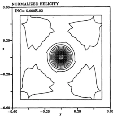
5.4 Normalized Helicity through a Lamb Vortex Core . . . .

6.1 Tangential Velocity Distribution for a Rankine Vortex . . . .

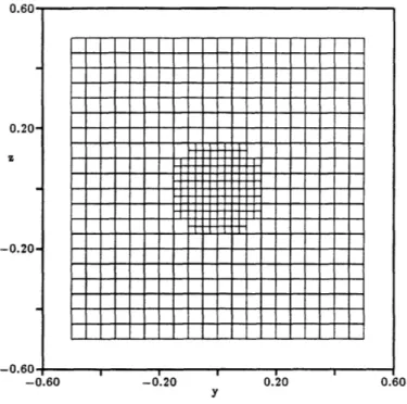
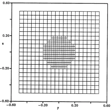
6.2 Tangential Velocity Distribution for a Lamb Vortex . . . . 6.3 Entropy Distribution for a Rankine Vortex . . . . 6.4 Entropy Distribution for a Lamb Vortex . . . . 6.5 Single Vortex- Initial Grid, y - z Slice ...

6.6 Single Vortex -6.7 Single Vortex -6.8 Single Vortex -6.9 Single Vortex -6.10 Single Vortex -6.11 Single Vortex -6.12 Single Vortex -6.13 Single Vortex -6.14 Single Vortex -6.15 Single Vortex -6.16 Single Vortex

-Initial Grid, a - z Slice . . . .

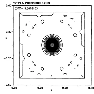
AP0 Contours at x = 0.0, Initial Grid.

APo Contours at x = 0.5, Initial Grid.

AP0 Contours at a = 1.0, Initial Grid.

AP0 Contours at z = 2.0, Initial Grid.

H, Contours at x = 0.0, Initial Grid .

HI Contours at a = 0.5, Initial Grid .

H, Contours at x = 1.0, Initial Grid .

H, Contours at z = 2.0, Initial Grid .

Adaptive Grid (1 level) based on APo, y

Adaptive Grid (1 level) based on APo, y

6.17 Single Vortex - Adaptive Grid (1 level) based on APo, y - z Slice at

z

.

. . .

. . . . .

- z Slice at a = 0.0

6.18 Single Vortex - AP0 Contours at az = 0.0, Adaptive

onAPo . . . .. . . ..

6.19 Single Vortex - APo Contours at z = 0.5, Adaptive on AP0 . . . .. . . .

6.20 Single Vortex - APo Contours at z = 1.0, Adaptive

onAPo

6.21 Single Vortex - APo Contours at az = 2.0, Adaptive onAPo ... . . . ...

6.22 Single Vortex - Adaptive Grid (2 levels) based z = 0.0 . . . .

6.23 Single Vortex - Adaptive Grid (2 levels) based z = 1.0 . . . .

6.24 Single Vortex - Adaptive Grid (2 levels) based z = 2.0 . . . .

Grid (1 level) Based

S.. . . .. . . . . .e

Grid (1 level) Based

Grid (1 level) Based

...

. . . . . . . . . . . . APo, y- z APo, y- z APo, y - z •. . . •.. . Slice Slice Slice

6.25 Single Vortex - APo Contours at z = 0.0, Adaptive Grid (2 levels) Based

on AP

6.26 Single Vortex - APo Contours at z = 2.0, Adaptive Grid (2 levels) Based

on APo

.

6.27 Single Vortex - Adaptive Grid (1 level) based on H,,, y - z Slice at x = 0.0 84

6.28 Single Vortex - Adaptive Grid (1 level) based on H,,, y - z Slice at

az

6.29 Single Vortex - Adaptive Grid (1 level) based on H,,, y - z Slice at az = 2.0 85

6.30 Single Vortex - H,, Contours at z = 0.0, Adaptive Grid (1 level) Based

6.31 Single Vortex - H, Contours at z = 1.0, Adaptive Grid (1 level) Based

onH

..

. . . .

.

. .

.

. . .

.

. .

.

. .

.

. . .

. .

. ..

6.32 Single Vortex - H, Contours at m = 2.0, Adaptive Grid (1 level) Based onH, . . . . ...

6.33 Single Vortex -Adaptive Grid (2 levels) based on H!, y - z Slice at x = 0.0 88

6.34 Single Vortex -Adaptive Grid (2 levels) based on H,, y - z Slice at x = 2.0 88

6.35 Single Vortex - APo Contours at a = 0.0, Adaptive Grid (2 levels) on H . . . . . ...

6.36 Single Vortex -APO Contours at x = 2.0, Adaptive Grid (2 levels)

on

H

. . .

...

Based

Based

6.37 Single Vortex - Convergence Histories for Adaptive Cases . . . .

6.38 Single Vortex - AP0 along Vortex Core for Adaptive Cases . . . .

6.39 Single Vortex - Convergence Histories for Varying v4 Cases . . . .

6.40 Single Vortex - AP0 along Vortex Core for Varying v4 Cases . . . .

6.41 Total Pressure Loss Contour at z = 1.20 for the NTF Delta Wing. . . .

6.42 Unequal Vortices -Initial Grid, y - z Slice . . . .

6.43 Unequal Vortices -Initial Grid, z - z Slice . . . .

6.44 Unequal Vortices -AP0 Contours at Inlet, Initial Grid . . . .

6.45 Unequal Vortices - APo Contours at Outlet, Initial Grid . . . .

6.46 Unequal Vortices - H, Contours at Inlet, Initial Grid . . . .

6.47 Unequal Vortices - HI Contours at Outlet, Initial Grid . . . .

89 89 90 90 91 91 92 101 101 102 102 103 103

6.48 Unequal Vortices - Adaptive Grid (1 level) based on APo, y - z Slice at

X = 0.0 . . . . 104 6.49 Unequal Vortices - Adaptive Grid (1 level) based on APo, y - z Slice at

Outlet . . . 104

6.50 Unequal Vortices - AP0 Contours at Inlet, Adaptive Grid (1 level) Based

on

A

Po

105

6.51 Unequal Vortices - APo Contours at Outlet, Adaptive Grid (1 level)

Based on APo . ... 105

6.52 Unequal Vortices -Adaptive Grid (2 levels) based on APo, y - z Slice at

Inlet . . . 106

6.53 Unequal Vortices -Adaptive Grid (2 levels) based on APo, y - z Slice at

Outlet . . . 106

6.54 Unequal Vortices -APo Contours at Inlet, Adaptive Grid (2 levels) Based

on A Po

.

.. ...

. ....

107

6.55 Unequal Vortices - APo Contours at Outlet, Adaptive Grid (2 levels)

Based on APo

107

6.56 Unequal Vortices - Adaptive Grid (1 level) based on H,, y - z Slice at Inletl 108

6.57 Unequal Vortices - Adaptive Grid (1 level) based on HI, y - z Slice at

Outlet . . . 108

6.58 Unequal Vortices - APo Contours at Inlet, Adaptive Grid (1 level) Based

on H . . . . 109

6.59 Unequal Vortices - APo Contours at Outlet, Adaptive Grid (1 level)

6.60 Unequal Vortices - H, Contours at Inlet, Adaptive Grid (1 level) Based

on H • . . . .. . . .

6.61 Unequal Vortices - HI Contours at Outlet, Adaptive Grid (1 level) Based

on

H

. . . ... .

Inlet . . . .

6.63 Unequal Vortices - Adaptive Grid (2 levels) based on Hn, y - z Slice at

O utlet . . . .

6.64 Unequal Vortices -APo Contours at Inlet, Adaptive Grid

onH, .. . . . . ...

6.65 Unequal Vortices - APo Contours at Outlet, Adaptive Based on H, ...

6.66 Unequal Vortices - Convergence Histories . . . .

6.67 Unequal Vortices -APo along Stronger Vortex Core . .

6.68 Unequal Vortices -AP0 along Weaker Vortex Core . . .

(2 levels) Based Grid (2 levels) . . . .• . . 110 110 111 111 112 112 113 114 114

List of Tables

2.1 Scaling Factors for Non-Dimensionalization . . . .

3.1 Nodes for Each Face, Trilinear Element . . . ..

6.1 Single Vortex - Comparison of AP0 Errors at Stations along Domain . .

6.2 Single Vortex - Comparison of AP0 Errors at Stations along Domain for

Varying v₄ . . . . . . . . . . . . . . . . . . . .. . . . . . . . . . . . . . .

6.3 Unequal Vortices - Comparison of AP0 for Stronger Vortex at Stations

along Dom ain .. ... ... ... .. ... ... ... ... .. ...

6.4 Unequal Vortices - Comparison of AP0 for Weaker Vortex at Stations

along Dom ain ... ...

6.5 Unequal Vortices - Comparison of AP0 Errors for Stronger Vortex at

Stations along Domain ...

6.6 Unequal Vortices -Comparison of AP0 Errors for Weaker Vortex at

Chapter 1

Introduction

The advent of parallel and vector supercomputers has placed computational fluid dy-namics in the forefront in the design and analysis of aerodynamic bodies. The ability to compute complex three-dimensional flowfields around all types of aircraft is now pos-sible. With these three-dimensional calculations the grids are usually fine enough to detect the relevant flow features such as shocks and vortices. However, with vortical flows, the truncation errors due to the grid resolution and the effects of artificial viscos-ity in the flow solver often result in large numerical errors which manifest themselves in the spurious diffusion of vorticity. One method that will reduce the numerical errors is to refine the computational grid around the vortical structures. The process of detect-ing a flow feature, markdetect-ing the region to be refined, and performdetect-ing the refinement or unrefinement of the grid is called grid adaptation. This thesis addresses the use of grid adaptation for vortex flows.

1.1

Background

In order to look at the effects of grid adaptation for vortex flows, an adaptive finite element algorithm for the Euler equations, developed by Dr. Richard Shapiro, was used [27]. The finite element flow solver was implemented in three dimensions using hexahe-dral elements. The advantage of using a finite element algorithm is that the method is "unstructured" by nature, thus lending itself to adaptive gridding where an unstructured grid is desirable, if not necessary. The advantage of using hexahedral elements is that they offer large CPU and memory reductions over tetrahedral elements. Shapiro [27] discusses three variations of the finite element method: the Galerkin method, the cell-vertex method (this method is the only method implemented in three dimensions and

thus is the method used in this thesis) and the central difference method. For a diverse range of papers on finite elements in fluids, the Proceedings of the Seventh International

Conference of Finite Element Methods in Flow Problems [5] is recommended.

Grid adaptation can be performed using three primary methods: grid redistribution, grid regeneration and grid enrichment. In the grid redistribution method, the mesh points in an initial computational grid are allowed to move as the solution proceeds. The survey article by Eiseman [10] is a good overview of various grid redistribution schemes. With grid regeneration either the entire computational grid or some portion of it is regenerated when adaptation occurs. This method of adaptation is described in articles by Peraire, et al. [20, 21]. Grid enrichment is a method in which additional nodes and elements are inserted into the grid. The survey article by Berger [4] presents a good overview of grid enrichment methods. The grid adaptation method used in this thesis is grid enrichment or grid embedding. Essentially, the adaptation algorithm divides a hexahedral element, more easily visualized as a cube, into eight smaller cubes.

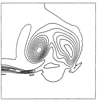
The focus of grid adaptation has predominantly been upon locating and refining shocks [27, 6]. As mentioned previously, the focus of this thesis is upon adaptation for vortex flows. The need for adaptation for vortex flows is demonstrated with an example from the calculations for the NTF delta wing performed by Becker [3]. The total pressure loss contours over the wing at x = 0.75 (Fig. 1.1), at the trailing edge X = 1.0 (Fig.

1.2), and in the wake x = 1.2 (Fig. 1.3), z = 1.5 (Fig. 1.4) and x = 2.0 (Fig. 1.5) show the diffusion of the primary vortex. The secondary vortex experiences an adverse pressure gradient and "bursts" close to the trailing edge. Although the secondary vortex bursts a region of high total pressure loss remains and drifts downstream [8]. Fig. 1.6 shows the total pressure loss along the streamline in the primary vortex core. The primary vortex forms at the leading edge and reaches roughly a constant value of total pressure loss of 0.6 about halfway along the wing. From this point to approximately 120% chord the total pressure loss is about constant. One would expect this behavior to continue for some distance downstream since the physical diffusion mechanisms are small. However, the total pressure loss at the outflow boundary is 0.417. This error is most likely due to the truncation error of the algorithm and the numerical dissipation

added to the algorithm for stability. It is the non-physical mechanisms of diffusion that can be reduced through grid adaptation.

Grid adaptation entails determining what flow parameter, called the adaptation parameter, best indicates a feature and then using this adaptation parameter to auto-matically mark the region of interest. Surprisingly, there has been little work in this area for vortical flows. Krist [15] uses a structured embedded grid formulation to resolve the vortical region for a 3-D delta wing. In Powell's ScD thesis [22], a non-adaptive grid embedding scheme was used to resolve the vortical regions for solutions of the coni-cal Euler equations. These are not adaptive schemes since the embedded regions are predetermined by inspection. Although they are approachs to refining the vortical re-gion, they lack the flexibility that is gained by automatic adaptation where the adapted region can expand or decrease as the solution evolves. Powell [23] also developed adap-tive methods for leading-edge vortex flows. One of his methods of adaptation used a refinement parameter based on numerics. The refinement parameter is a measure of mesh-convergence, constructed by comparison of locally coarse and fine grid solutions. When a cell has been refined, the solution at the center of one of the sub-cells is com-pared to the solution at the same point based on the coarse cell. When the refined

value on the fine grid is the same as the coarse grid value, the solution is locally mesh-converged. The advantage of using a refinement parameter based numerics is that any region requiring refinement is detected. The other adaptation indicator Powell used was total pressure loss [23]. Batina [2] also chose to use total pressure loss as an adaptation indicator for vortex flows.

This thesis examines two flow parameters as adaptation indicators for vortex flows: total pressure loss and normalized helicity. In addition, the gradients of these parame-ters are examined to determine if they are better indicators than the quantities alone. Finally, a method by which cells are automatically marked for refinement and unre-finement is desired, this is called automatic thresholding. The automatic thresholding algorithms of Dannenhoffer [6] and Powell [23] are evaluated for the test cases in this thesis and an automatic thresholding algorithm is determined.

1.2

Overview of thesis

First the governing equations for a compressible, inviscid flow (the Euler equations) and the physical boundary conditions are described in Chapter 2. Chapter 3 defines some fundamentals of the three-dimensional finite element method used in this the-sis. Chapter 4 presents a complete description of the solution algorithm and discusses many implementation issues. The spatial discretization, implementation of the bound-ary conditions, smoothing, and time integration scheme are the essential components of the solution algorithm described in this chapter. The requirements for consistency and conservation are also mentioned at the end of this chapter. The focus of this thesis is upon adaptation for vortex flows and in Chapter 5 the adaptation procedure is de-scribed. The adaptation criteria for vortex flows is discussed along with a description of the quantities to be adapted upon, a brief discussion of the possible use of gradients of these quantities, and a method to automatically choose the upper and lower limits for cell refinement and unrefinement. Chapter 6 then describes the vortex flow results. First the vortex core models are described. Next, the results from the two test cases are detailed. The test cases are a single vortex and two vortices of unequal strength with opposite rotation directions. Some conclusions of this research are then given in Chapter 7.

Figure 1.1: Total Pressure Loss Contour at x = 0.75 for the NTF Delta Wing

Figure 1.3: Total Pressure Loss Contour at z = 1.20 for the NTF Delta Wing

Figure 1.5: Total Pressure Loss Contour at x = 2.00 for the NTF Delta Wing

0.000 0.313 0.625 0.938 1.250 Length

1.563 1.875 2.188 2.500

Figure 1.6: Total Pressure Loss along the Primary Vortex Core for the NTF Delta Wing (Length = 0 is the leading edge, Length = 1.0 is the trailing edge and Length = 2.0 is the downstream boundary)

Chapter 2

Governing Equations

This chapter describes the governing equations for the flow of a compressible, inviscid, ideal gas including the assumptions on which they are based. The set of equations rep-resenting conservation of mass, momentum, and energy describing this flow are termed the Euler equations. Additionally, in this chapter the non-dimensionalization of the equations will be discussed, and the physical boundary conditions will be described.

2.1

Euler Equations

The Euler equations for a three-dimensional flow consist of five partial differential equa-tions representing conservation of mass, conservation of momentum (one for each com-ponent of momentum), and conservation of energy. In order for the Euler equations to describe the flow of a compressible, inviscid, ideal gas, the following assumptions are necessary:

* The fluid is a homogeneous continuum;

* There is no viscosity;

* There is no heat transfer (non-conducting); * The fluid obeys the ideal gas law.

Another assumption made in this thesis is that the body forces are zero. Although the Euler equations are not exact for any real flow, they are a good approximate model for many problems of interest. In this thesis the steady-state solution is sought. In

order to achieve the steady-state solution, a time marching scheme is used, thus the unsteady Euler equations are described here.

The three-dimensional unsteady Euler equations in Cartesian coordinates can be written in vector form as

OU OF 0G 0H

--

+

T

-ý-

+

=0

(2.1)

Z y Oz

where the state vector U p Pu pv Pt, pw pE

and the flux vectors F, G and

fnu Pu2 _{+ p} Pu?) put' puH

I

V

where p is density, u, v, and w are the flow velocities in the z, static pressure, E is total energy per unit mass, and H is the mass, given by the thermodynamic relation

(2.2)

y, and z directions, p is total enthalpy per unit

H = E

+

.

(2.3)

An equation of state is used to close the system of equations. Under the assumption of an ideal gas, the perfect gas law, p = pRT, eliminates temperature from the definition of E = c,T + ] (u2 + v2+ W2) and yields the closing relation

P=

( -

1)(E

-

1

(U2

+

+

p

2

(2.4) where the specific heat ratio 7- is equal to 1.4 for air and is constant for all calculations performed.

2.2

Non-Dimensionalization

It is usually convenient to non-dimensionalize the governing equations for a problem since this makes the solutions independent of any particular system of units, clarifies

H are P

defined by:

Variable Factor Freestream Value u, v,

w

--t

L/al

-D-Table 2.1: Scaling Factors for Non-Dimensionalization

the scales important to the problem and can reduce the sensitivity of the solution to round-off errors. Table 2.1 lists the scaling factors and freestream values for each of the variables in the Euler equations. It can be seen that the important non-dimensional flow parameters are the freestream Mach number, M., and 7. Non-dimensionalization does not change the form of the equations, but does alter the form of the freestream boundary conditions.

2.3

Auxiliary Quantities

The following is a list of relevant auxiliary quanitities that can be defined in terms of the primitive variables:

Local speed of sound: a7=p VP

Mach Number:

Total Pressure:

Total Pressure Loss:

uM = 2 + v2 + w 2 a Po = p(l + 2 1 M2) Poo-Po

Poo

Entropy: AS = log

7-P't

where the freestream entropy is defined to be zero. As mentioned previously, normalized helicity is used as one of the adaptation quantities. The normalized helicity is defined as:

H,,

. -

I

_(I[TII

where

V

2.4

Physical Boundary Conditions

Boundary conditions must be specified in order to solve for any system of differential equations. The problems addressed in this thesis use only farfield boundaries; how-ever, solid wall boundary conditions also have been implemented and are discussed in Appendix A. The implementation of the farfield boundary conditions is discussed in Section 4.3.

The farfield boundary conditions are based on quasi-one-dimensional characteristic theory. The three-dimensional Euler equations are transformed into a system based on coordinates normal and tangential to the boundary. The transformed directions will be denoted by (n, t, b), where n is normal to the boundary (positive pointing inward) and

t and b are tangential to the boundary. Assuming that there are no variations in the t and b directions, i.e., the derivatives tangential to the boundaries are neglected, this

reduces the three-dimensional Euler equations to a one-dimensional system of equations. Manipulation of the resulting unsteady, inviscid one-dimensional Euler equations yields

the following near-diagonal system of equations [12] ut un 0 0 0 0 Ut Ub 0 un 0 0 0 Ub 0 0

S

+

0 0

un

0

0

=0

(2.6)

+

where S is the entropy, Un is the velocity normal to the boundary, ut and Ub are the

velocities tangential to the boundary, and

J+

(2.7)

2a

=

n

.

(2.8)

The system is diagonalized by assuming locally isentropic flow. For the vortex cases used the flow is not locally isentropic; however, an analysis of the off-diagonal and diagonal terms showed that the off-diagonal terms are small. Therefore, dropping these terms results in a good approximation and decouples the equations. Thus the characteristic equations are

a J+

8aJ

t+ (u, + a)

-

_0,

OJ

OJ

--

+ (

_Un

_-

_a)

_--

_01,

_(2.10)

Out _Fut Unt _Out

(2.11)

-

+

un"-

=

0,

(2.2)

Ot

On

aus

Bus

Oub _OS Oub_OS

- + UnT

=

0.

(2.13)

The characteristic variables ut, ub and S are convected normal to the boundary at velocity un, while J+ is convected normal to the boundary at velocity un + a and J_ is convected normal to the boundary at velocity un - a. Therefore, if 0 < un < a, the boundary is a subsonic inflow boundary, so J+, S, ut and ub propagate into the domain, while JL propagates out of the domain. A subsonic outflow boundary exists

when -a < u, < 0 in which case J+ is specified from the exterior of the domain

and the other chacteristics come from the interior. At a supersonic inflow boundary,

un > a, all the characteristics are entering the domain and thus must be specified. For

a supersonic outflow boundary, un < -a, all the characteristics propagate out of the domain, therefore, nothing must be specified.

Chapter 3

3-D Finite Element Concepts

This chapter will describe some of the important concepts of the three-dimensional finite element method used in this thesis. For a broader overview of finite element methods in both two and three dimensions for the Euler equations, the work of Shapiro [27] is highly recommended. The following finite element description is based upon that work. This chapter will focus strictly on 8 node, 3-D trilinear elements. The terms element, node,

edge and face are defined, and the transformations between physical and computational

space are described. A brief discussion of the derivative calculation is also given.

3.1

Terminology

When using numerical methods, the physical domain of interest must be discretized in some fashion. In the finite element method the physical domain is subdivided into

elements, each of which is composed of some number of nodes. In this thesis, the physical

domain, which is three-dimensional, is subdivided into hexahedral elements each with

8 nodes. A hexahedral element will have 6 faces and 12 edges. Figure 3.1 illustrates a

3-D element showing the faces, edges and nodes.

The advantage of hexahedral elements is that a hexahedral mesh will have roughly five times less elements than a tetrahedral mesh. This results in significant savings in

CPU time and memory since many operations are performed on elements. The

disad-vantages of hexahedral elements are that during grid generation hexahedral elements may be more difficult to fit to a geometry and with grid adaptation special treatment must be given to the nodes at the interface between the coarse grid and the fine grid. Specifically, at the interface the new nodes generated from grid adaptation will have

Face

Edge

Node

Figure 3.1: 3-D Finite Element

to be interpolated from the coarse grid and conservation should be maintained on the new adaptive grid. The treatment of the interface will be discussed in Section 5.1. The difficulty of fitting hexahedral elements to a geometry can be circumvented since the finite element method allows degenerate elements where a degenerate hexahedron will result in a prism. Figure 3.2 a shows degenerate hexahedra.

Figure 3.2: 3-D Degenerate Finite Element

In the finite element method, all operations are performed at the elemental level, with element contributions distributed to the nodes. The finite element is unstructured in nature. It is not necessary for each grid point to be indexed by (i,

j,

may belong to any number of elements.

I

I

I

3.2

Finite Element Discretization

The finite element discretization will be described in three dimensions. The finite el-ement method provides a way to make a convenient transformation between a local, computational space (natural coordinates) and a global, physical space. The natural coordinates will be denoted by (ý, 77, () and the physical coordinates will be denoted by

(z, y, z). Figure 3.3 shows a typical 3-D finite element with the directions of the natural

coordinates.

C

(-i.-1.-1)

Figure 3.3: Natural Coordinates

In the finite element discretization one assumes that within each element, some quantity q(e) is determined by its nodal values qi and a set of shape or interpolation

functions NMe). Typically, the interpolation functions are chosen to be polynomials in

the natural coordinates. The quantity, q(e), is then given by q(Eq)(•, = _{1t (,j771}

i=1

(3.1)

where the summation is over the nodes of the element. Similarly, the geometry of the element is interpolated in terms of nodal coordinates, i.e.,

(3.2)

,(e)(ý, 7,

C)

=

8 =e@

ib()

yjNj(•,,7,5),

(3.3)

(3.5)

where zi, yi and zi are the coordinates of node i in element e and the sum is taken over the eight nodes.

The element shape functions are summed to give global shape functions Ni, so that globally q can be written

M

q(oy,z)=

Ni(oyz)qi,

(3.6)

i=1

where M is the total number of nodes in the mesh. The relation between NM )(,)

C)

3.2.1 Interpolation Functions

The interpolation functions N(e) must have certain properties for the finite element ap-proximation to be valid. The following lists the properties of the interpolation functions used in this thesis:

1. The interpolation function NMe) must be 1 at node i and 0 at all other nodes of

the domain. This is required so that Eq. (3.6) can hold for each node.

2. The interpolation function N(e) is 0 outside of the element e. This holds for a local finite element approximation. Ag a result of this property the global shape function Ni(z, y, z) at node i is the sum of the elemental interpolation functions

Ne)((,

C,)

3. In each element, the sum of all the nodal interpolation functions Ný() are

identi-cally 1 at each point (7, (, ) in the element. This is required for consistency in the approximation.

3.2.2 Derivative Calculation

The derivative of a quantity in terms of the nodal values of that quantity is often desired. In order to calculate the derivatives in physical space, the Jacobian of the transformation is required. This is seen below:

aq

Oq

Oq

* DC

ay

where J is the Jacobian matrix

J =

"' 0

8N(e)

ON(e)

e

,f

z

z

DN e)

zi

(3.8)

Once J has been assembled, J-1 can be calculated, so the derivatives of a quantity

q in each element can be computed as follows: " Oq(e)

0q(e)

Dq(e)

" z

8N}')

8

.(e)O

Eqj0NiVe)

•

087

DC

(3.9)

where the qi are the nodal values of q.

(1,1,1)

77

4

1 2

3

Physical Coordinates Natural Coordinates

Nodes in bold, Faces in italic

Figure 3.4: Geometry of Three-Dimensional Element

3.3

Trilinear Elements

The 8-node, three-dimensional element shown in Fig. 3.4 is a trilinear element. To help clarify this figure, Table 3.1 lists the nodes that make up each face of the element. The interpolation functions for a trilinear element are

NI = (1 - )( -

7)(1

(3.10)

(3.11)

(3.12)

Table 3.1: Nodes for Eaclb Face, Trilinear Element

Face Nodes on Face

Face Nodes on Face

1 1-2-3-4 4 6-7-3-2 2 8-7-6-5 5 4-3-7-8 3 1-5-6-2 6 1-4-8-5 5

(-1,-1,-1)

8

1

7

It will be convenient to

•

=

~=

z(W, 7, 0) =

expand Eqns. (3.1)

-

(3.4) as follows:

a, +a2 + a3 + a4C•+

a56

a6C

+

a7•C +

a86s7C,

b, + b26 + b371 + b4C + b&7 + b6 7 b 8(+b ,0

C1

+

C

+

C377

+

C4

+

CS'q

+

C677 + C

.C

+ cs8C,

di

+

d2+

d4C

+

ds67

+

d67

+

d76( + ds6r},

where

di

=

(

q

+

q2

+

+

+

qs

+ q6 +

+

qs)/8,

(3.22)

(-ql + q

+ q3 - q4 - qs + q +q7 - qs)/8,

(3.23)

+q8)/8,

(3.24)

+

+

+

-

(3.25)

ds=

(

(3.26)

(

(

+

+

(3.28)

d8

= (-ql

+

q2 - q3 +

+ q5 -6 +7 -q8)/8.

(3.29)

The coefficients a0, bi, and ci are determined by the same equations as above except

with the q,'s being replaced by zj's, yj's, aid zi's, respectively. The Jacobian matrix

can be calculated by using Eq. (3.8). The three-dimensional Jacobian J is

a

+

as7+

+

ag1C b

+ bsl

+

bs

+

bs7C c

+ cs5 + c + cs87(

J = a3+

ajs

b•~

be6C(+

a

+

ae67

+

+ asft

b

+

+

b

ý

+

b

W

c677+

where ai, bi, and ci are the coefficients in the expansions of z, y, and z in the element.

(3.13)

(3.14)

(3.15)

(3.17)

(3.20)

(3.21)

Chapter 4

Solution Algorithm

This chapter describes the 3-D finite element algorithm used to obtain the steady-state solution of the Euler equations as developed by Shapiro [27]. An overview of the algorithm will first be described. The spatial discretization of the finite element method will then be described. The term "finite element method" is actually quite broad in meaning, the selection of the test functions results in quite different methods. For the 3-D calculations presented in this thesis a "cell-vertex" finite element method was used. The spatial discretization and test functions used for the cell-vertex finite element method is described within Section 4.2. The implementation of the boundary conditions is then discussed. Artificial viscosity is required for stability and is discussed in Section 4.4. Section 4.5 will then describe the time marching scheme. It should be noted here that the time marching scheme is not time accurate. Finally, consistency and conservation are briefly discussed.

4.1

Overview

The steady-state solution is obtained from the unsteady Euler equations by using a time marching technique. First, an initial condition must be imposed, then the solution is corrected by an iterative technique that resembles the solution of the unsteady problem until some level of convergence is achieved. The iterative technique used is a four-stage time integration scheme which essentially consists of the following steps: The boundary conditions are applied before each step in the multistage scheme. Then, a summation of the fluxes over the element volume is calculated. Next, artificial viscosity is computed during the first stage of the integration and "frozen". The artificial viscosity is then added to the flux summation and this quantity is termed the residual. The residual

then represents the difference between the current step and the previous step. Finally,

the current solution is updated to obtain.the next approximation. This process is

then repeated four times. The entire process is repeated until some desired level of

convergence is achieved. Convergence is signalled when the RMS of all changes divided

by the RMS of all the state vectors is less than some specified value, typically around

10-6.

4.2

Spatial Discretization

The conservation form of the Euler equations ( Eq. (2.1) ) is used for spatial

discretiza-tion and is written as

0U

OF

OG

OH

-- + ~-

+ -

+--

=0

(4.1)

z y

Oz

where U is the state vector and F, G and H are the flux vectors in the z, y and

z

directions. Within each element the state vector U(e) and flux vector F(e), G(e) and

H(e) are written

u(e) = N

(')U,

(4.2)

F(e)

ZN(e)F-,

(4.3)

G(e) =

ZN(')G-,

H(e) = ZN(e)H, (4.5)

where Ui, Fi,

Gi

and Hi are the nodal values of the state vector and flux vectors, and

NMe) is the set of interpolation functions for element

e.

The derivatives of these expressions can be computed by the method described in

Section 3.2. The formula for the derivative in each element in terms of the nodal values

follows:

BU(*)dd

OU(e=

OF(') ON(e) -

Z

F(4.7)

OG()=

Gi(4.8)

Oz

Hi

(4.9)

where the summation is over the nodes i of element e. Summing over all of the elements

in the domain results in the following equation:

dU _ ON, ON, ON,

N- -- Fi - - H- (4.10)

dt Ox 8Y

Oz

where Ni is the sum of the interpolation functions of node i for each element that

contains node i. It should be noted here that Ni is now a global row vector and dUi/dt

is a column vector. These vectors are of length M, where M is the total number of

nodes in the mesh.

Equation (4.10) does not hold for all points in space since the derivatives of the

interpolation functions do not exist for all points in space. Instead of asking for an

equation that holds at each point we need an equation that holds for each function [28].

The right form needed is the weak form of the equations. The weak form minimizes the

error in the discretization by having the error orthogonal to the space spanned by a new

of nodes. The weak form of the equation now holds for each test function. To create

the weak form, premultiply Eq. (4.10) by

f

and integrate over the entire domain.

Because we are integrating over the entire domain, this allows for the introduction of

discontinuous solutions as well as providing some means for obtaining the nodal values

of the unknowns. The weak form of Eq. (4.10) is

Mid = - (J F NJ+G+ +NJ

'y'y(4.11)

where Mi

is the consistent mass matrix. and is determined as follows

This results in the semi-discrete equation

dUt

dty

where R,, R. and R, are the residual matrices. The matrices M, R,,, RY and R,

involve the integration of quantities over all elements in the domain. These integrations

are performed at the elemental level in natural coordinates and are assembled to give

the global matrices.

At this point the choice of test functions and resulting methods from each choice will

be discussed. Shapiro [27] discusses three choices of test functions in two dimensions

that result in the Galerkin method, the cell-vertex method and the central difference

method, all of which fit into the "finite element method". The test functions for the

Galerkin method are chosen to be the same as the interpolation functions, for the

cell-vertex method the test functions are chosen to be a constant, and for the central

difference method the test functions can be set to a series of Dirac delta functions. The

Galerkin and cell-vertex methods were shown to be both more robust and

computa-tionally efficient than the central difference method. The cell-vertex method was less

computationally expensive than the Galerkin method, although this could be due to

optimizations in the residual calculation within the cell-vertex method. In three

dimen-sions, only the cell-vertex was implemented. For trilinear elements, the test functions,

fy

),

for each node within each element were chosen to be 1/8.

The calculation of each residual matrix is identical, therefore, only the calculation

of the R., matrix will be shown here. The calculation of the R, matrix begins with

R1f

j

-yf

;

dz

dy dz,

(4.14)

using Eq. (3.9) " and

de

dydz translatedinto natural coordinates become

(

J 9, +

N

15

Ozs

Ofs

ON

,

3

(.15

d dydz

=

lJj

dfd

dC.

(4.16)

Thus, the

R.

matrix expressed in natural coordinates is

RQf

-

+

ON-)

The inverse of J can be expressed as

7J-

=

(4.18)

where J* is the adjoint of J [29]

.

Substituting this formula into Eq. (4.17) yields

.'

1

_'

_.

_ON

_{_,oN}

_ON

RX= jjj

+ J1,

-

) d) d dC.

(4.19)

For the mass matrix, all the quantities being integrated are also polynomials. Thus, all

the element integrals can be done analytically, resulting in a significant savings in CPU

time. (Note: in the implementation the element integrals are computed exactly using

MACSYMA since hand generation is prone to mistakes.)

The nodal values of the state vector are solved using Eq. (4.13). The mass matrix

M is a sparse, positive definite matrix, but is unstructured making it computationally

expensive to invert. In this thesis, we are only interested in the steady-state solution;

therefore, M can be replaced by a "lumped" (diagonal) matrix, ML, where each diagonal

entry is the sum of all the elements in the corresponding row of M. This allows Eq.

(4.13) to be solved explicitly, thus inexpensively. For the test functions chosen, the

lumped mass matrix has a value along the diagonal equal to 1/8 of the cell volume.

4.3

Boundary Conditions

Before discussing the implementation of the boundary conditions, several definitions are

needed for clarity. First, a face of an element can exist in the interior of the domain or

along a boundary (a solid boundary may exist in the interior of the domain such as with

a planform of a wing). The boundary face of an element can either be a solid boundary

face or a farfield boundary face. The types of boundary faces and boundary nodes an

element can have and the types of boundary nodes that can exist on each boundary face

are summarized below.

* Boundary face types: solid, farfield

. Possible nodes on a solid face: solid, farfield, corner

* Possible nodes on a farfield face: farfield

Farfield faces are the simplest faces since they can only contain farfield nodes. The

implementation of solid wall boundary conditions is discussed in Appendix A.

The implementation of the farfield boundary conditions will now be described. As

discussed in Section 2.4, the farfield boundaries are based on one-dimensional

charac-teristic theory. For farfield boundaries, the inward pointing unit normal vector f and

the two unit tangent vectors

i

and b must be computed. First, the normal vector must

be computed. This is computed as follows:

1. Loop over all elements in the domain.

2. Identify any farfield faces on each element.

3. Determine the farfield node numbers on the farfield face.

4. Compute the normal vector components, i.e. n,, ny, nz, by taking the components

of the cross product of the diagonals of the face.

5. Sum the normal vector components of all faces that contain the farfield node i .

6. Normalize the components by the magnitude of the normal vector, fi.

The normal vector is computed the same for all farfield nodes. The tangential velocity

vector can now be computed using the following formula

V = V - (V. *)i. (4.20)

The unit tangent vector is then determined by

Vt _(4.21)

If the tangential velocity is zero, then an arbitrary tangential vector is chosen. The

other unit tangential vector

&

is calculated by taking the cross product of i and i.

The 1-D Riemann invariants and the corresponding wave speeds are now defined

using the above vectors

2a

2a

-1 -

Un

Un

-a

P

P7

where u, = n.if,

ut

V.t

. b.

each point on the boundary. This is done using the updated values of the state vector of

the nodes along the boundary. Then for each point on the boundary, the characteristics

are calculated using the solution state vector U and the freestream state vector Uo.

Next, a decision is made based upon the sign of the wave speeds whether to use the

invariant based on the interior state vector or the freestream state vector. If the wave

speed is positive then the characteristic based upon the freestream state vector is used.

The invariants are transfomed back into primitive variables, and these primitive

variables are then used to calculate the fluxes at the boundary nodes in the residual

calculation. The primitive variables are calculated as follows:

1 un = (CI - C2),

(4.23)

a =

-1(C1

+

),

(4.24)

4

2

p = pa,

(4.26)

7

V

= un,n + C

t, + COsb,

(4.28)

+

+

H

+

1(U

_{+ V}

_{+ W2),}

_(4.30)

H

-y-

1p

2

where C

-

C

are the characteristic variables above. The characteristics are also used

to update the state vector at the beginning of each iteration.

4.4

Smoothing

Artificial viscosity is added in order to stabilize the numerical scheme as well as damp out

background disturbances. The smoothing used consists of a pressure-switched second

difference term and a fourth difference term, similar to that discussed by Rizzi and

Erikson [25]

.

A Laplacian-type of second difference is used due to the unstructured

nature of the grids. The smoothing is based essentially on the calculation of an elemental

contribution to a second difference. The second difference smoothing method suggested

by Ni [19] is used. This method is relatively fast, conservative and robust, but gives

a non-zero contribution to the second difference for a linear function on a non-uniform

grid, resulting in first-order accuracy. Thus, the right-hand side of Eq. (4.13) will have

a non-zero contribution due to the second difference [17].

4.4.1

Second Difference Smoothing

Figure 4.1 shows the contribution of a typical element to the second difference at node

1. The numbers inside the box are the node numbers, the numbers outside are the

weights, denoted wi for node i. The contribution from an element to a node is obtained

by subtracting the value at the node from the average value in the element. The second

difference at a node is then the sum of the esntributions from all elements that contain

node i. That is, the contribution to the second difference at node 1 from element e is

V(e)=k(e)(

U+U2+U3+U4

Us+U6+U7+U$

-U)

(4.31)

or equivalently expressed using the weights

8

V = k(e) -(s) w' U (4.32) i=-1