HAL Id: hal-00473820
https://hal.univ-brest.fr/hal-00473820
Submitted on 19 Apr 2010
HAL is a multi-disciplinary open access
archive for the deposit and dissemination of
sci-entific research documents, whether they are
pub-lished or not. The documents may come from
teaching and research institutions in France or
abroad, or from public or private research centers.
L’archive ouverte pluridisciplinaire HAL, est
destinée au dépôt et à la diffusion de documents
scientifiques de niveau recherche, publiés ou non,
émanant des établissements d’enseignement et de
recherche français ou étrangers, des laboratoires
publics ou privés.
experiment KEOPS (Kerguelen Islands, Southern
Ocean)
Fanny Chever, Géraldine Sarthou, Eva Bucciarelli, S. Blain, Andrew Bowie
To cite this version:
Fanny Chever, Géraldine Sarthou, Eva Bucciarelli, S. Blain, Andrew Bowie. An iron budget during the
natural iron fertilisation experiment KEOPS (Kerguelen Islands, Southern Ocean). Biogeosciences,
European Geosciences Union, 2010, 7, pp.455-468. �hal-00473820�
© Author(s) 2010. This work is distributed under the Creative Commons Attribution 3.0 License.
An iron budget during the natural iron fertilisation experiment
KEOPS (Kerguelen Islands, Southern Ocean)
F. Chever1,2, G. Sarthou1,2, E. Bucciarelli1,2, S. Blain3,4, and A. R. Bowie5 1Universit´e Europ´eenne de Bretagne, 35000 Rennes, France
2Universit´e de Brest, CNRS, IRD, UMR 6539 LEMAR, IUEM; Technopˆole Brest Iroise, Place Nicolas Corpernic,
29280 Plouzan´e, France
3Laboratoire Oc´eanographie Biologique de Banyuls sur Mer, Universit´e Pierre et Marie Curie, Paris 06, quai Fontaul´e,
66650 Banyuls sur Mer, France
4Laboratoire Oc´eanographie Biologique de Banyuls sur Mer, CNRS, quai Fontaul´e, 66650 Banyuls sur Mer, France 5Antarctic Climate and Ecosystems Cooperative Research Centre (ACE CRC), University of Tasmania, Hobart, Australia
Received: 29 May 2009 – Published in Biogeosciences Discuss.: 10 July 2009 Revised: 5 January 2010 – Accepted: 12 January 2010 – Published: 2 February 2010
Abstract. Total dissolvable iron (TDFe) was measured in the water column above and in the surrounding of the Kergue-len Plateau (Indian sector of the Southern Ocean) during the KErguelen Ocean Plateau compared Study (KEOPS) cruise. TDFe concentrations ranged from 0.90 to 65.6 nmol L−1
above the plateau and from 0.34 to 2.23 nmol L−1
off-shore of the plateau. Station C1 located south of the plateau, near Heard Island, exhibited very high values (329– 770 nmol L−1). Apparent particulate iron (Feapp), calculated
as the difference between the TDFe and the dissolved iron measured on board (DFe) represented 95±5% of the TDFe above the plateau, suggesting that particles and refractory colloids largely dominated the iron pool. This paper presents a budget of DFe and Feapp above the plateau. Lateral
ad-vection of water that had been in contact with the conti-nental shelf of Heard Island seems to be the predominant source of Feappand DFe above the plateau, with a supply of
9.7±3.6×10⁶and 8.3±11.6×10³mol d−1, respectively. The residence times of 1.7 and 48 days estimated for Feapp and
DFe respectively, indicate a rapid turnover in the surface wa-ter. A comparison between Feapp and total particulate iron
(TPFe) suggests that the total dissolved fraction is mainly constituted of small refractory colloids. This fraction does not seem to be a potential source of iron to the phytoplank-ton in our study. Finally, when taking into account the lat-eral supply of dissolved iron, the seasonal carbon sequestra-tion efficiency was estimated at 154 000 mol C (mol Fe)−1,
Correspondence to: G. Sarthou
(geraldine.sarthou@univ-brest.fr)
which is 4-fold lower than the previously estimated value in this area but still 18-fold higher than the one estimated dur-ing the other study of a natural iron fertilisation experiment, CROZEX.
1 Introduction
Iron (Fe) is essential for the growth of marine phytoplankton (Sunda, 1989), and plays an important role in biochemical re-actions such as photosynthesis and nitrate reduction (Rueter and Ades, 1987; Kutska et al., 2002). Artificial and natural Fe fertilisations in High Nutrient Low Chlorophyll (HNLC) regions of the World’s oceans have shown that iron inputs enhance phytoplankton growth and partly control the major biogeochemical cycles of elements important for Earth’s cli-mate (Boyd et al., 2000; Coale et al., 2004; Blain et al., 2007; Pollard et al., 2009). However, many uncertainties exist fol-lowing such fertilisation experiments, for example the carbon sequestration efficiency, i.e. the amount of carbon exported to the deep ocean per unit iron added.
Moreover, the biogeochemical cycle of iron is still not well understood. This is partly due to its complex physico-chemical speciation. Iron exists in different forms and the availability of these forms to phytoplankton is not well es-tablished (Bruland and Rue, 2001). The physical speciation is operationally defined as the partitioning between dissolved iron (DFe, < 0.2 µm) and particulate iron (PFe, >0.2 µm). Although particulate fraction may be the dominant pool of total iron in the water column (de Baar and de Jong, 2001), the majority of the studies had focused on the dissolved phase
which is thought to be a proxy for the bioavailable form (Frew et al., 2006; Morel et al., 2008). Exchanges between the different physical pools of iron take place in seawater, and an understanding of the distribution of iron in those pools, as well as of the fluxes between them is needed to better con-strain the iron cycle in the ocean (Frew et al., 2006). Only a few studies have shown that part of the particulate iron may be used by phytoplankton (Johnson et al., 2001; Maldonado et al., 2001). Small-particles below the defined colloidal size range (0.02–0.2 µm; Wu et al., 2001), and included in the dissolved phase, have also been considered to be a possi-ble bioavailapossi-ble form of iron to phytoplankton although less available than the truly soluble iron (Wu et al., 2001).
Acidified unfiltered samples allow the determination of to-tal dissolvable iron (TDFe). That fraction represents the sum of the dissolved iron (i.e. the labile dissolved iron which is the fraction that is released after a few days of acidification) plus the refractory colloidal iron (i.e., that fraction that dis-solved after more than a few days of acidification) plus the fraction of particulate material that dissolves during extended (>6 months) acid storage (iron adsorbed on lithogenic or bio-genic particles, contained within biobio-genic particles and labile lithogenic particulate iron) (de Baar et al., 1999; L¨oscher et al., 1997; Bowie and Sedwick, 2004). In the literature, the set of TDFe observations is much smaller than that of DFe. Studies of TDFe can however give important informa-tion about the iron cycle, notably on the sources of iron to the ocean. Indeed, lithogenic material deposited on continental shelf sediments and atmospheric dust inputs, which are the most important Fe sources in the surface waters of the open ocean, have been correlated with elevated concentrations of TDFe (Jickells et al., 2005; Elrod et al., 2004; Sarthou et al., 1997; Sedwick et al., 2008; Croot et al., 2004).
During the KEOPS (Kerguelen Ocean and Plateau com-pared Study) cruise, a multi-tracer approach was used to identify and quantify natural iron fertilisation over the plateau. DFe (>0.2 µm) was analysed on board and it repre-sented the labile dissolved iron (i.e., soluble Fe and colloidal Fe dissolving after a few days of acid storage). The study of this fraction clearly demonstrated the existence of a dis-solved iron-rich reservoir above the plateau below the mixed layer (Blain et al., 2007). At the date of the cruise (January– February 2005), DFe enrichment was partly due to inputs from the sediment above the plateau and/or to regeneration of biogenic particles. Predominant mechanisms allowing DFe transport into surface waters were shown to be diapycnal dif-fusive flux and winter mixing (Blain et al., 2008). However, other geochemical tracers have suggested that the dissolu-tion of lithogenic material transported over the plateau by lateral advection might also be a source of iron to this region (Zhang et al., 2008; van Beek et al., 2008; Jacquet et al., 2008). Additionally, Park et al. (2008a) showed that the flow over the shallow platform in the eastern side of the plateau is consistently northwestward. This feature is strongly sup-ported by depth-averaged (over the first 500 m depth)
time-mean currents directly measured by one-year-long current meter moorings at 2 stations (located above the plateau at 50.2◦S/72.3◦E and 49.5◦S/73.0◦E), as well as by repeated
LADCP measurements at A3 and C11. A transport of iron from Heard Island to the plateau should thus be possible.
The present work focuses on the distribution of TDFe above the Kerguelen plateau and in the surrounding waters, and uses this parameter as an additional tracer to better con-strain the Fe cycle in a naturally fertilised area. A budget of DFe and Feapp for the region located above the plateau is
presented and the fluxes exchanged between these two pools are calculated.
2 Material and methods 2.1 Study area
During the KEOPS cruise (18 January to 13 February 2005), three transects were studied (A, B and C). Seven stations lo-cated above the Kerguelen plateau (A3, B1, B3, B5, B7, C1 and C5; water depth from 150 to 607 m) and two stations lo-cated outside the plateau (B11, C11; water depth >3000 m) were sampled for TDFe (unfiltered samples) (Fig. 1).
The hydrology and the circulation around and above the Kerguelen Plateau have been described by Park et al. (2008a, b). Briefly the Kerguelen Plateau constitutes a barrier to the eastward flowing Antarctic Circumpolar Current (ACC). Most of the ACC is deflected north of the Kerguelen Islands but a remainder passes between the Kerguelen Islands and Antarctica. Above the plateau, the remainder of the ACC comes from the western part of the plateau (see Fig. 1). Cur-rents travel along the western flank of the plateau, passing south and east of Heard Island, before riding up above the plateau. South of the plateau, a branch of the Fawn Trough Current (FTC) flows toward the north along the eastern flank of the plateau (near stations B11 and C11).
2.2 Sampling and analyses
Samples were collected with acid-cleaned 12 L Go-Flo bot-tles mounted on a Kevlar cable. All sampling was carried out in a clean-room container. Unfiltered samples were collected in acid-cleaned 125 mL high density polyethylene (HDPE) bottles and immediately acidified with ultrapure hydrochlo-ric acid (HCl, Merck, 250 µL, final pH 1.7). Samples were stored at room temperature and analysed 18 months later in the shore-based laboratory (LEMAR, Brest, France), in order to release the most refractory Fe species into the dissolved form (L¨oscher et al., 1997; Bowie and Sedwick, 2004).
TDFe analyses were performed by flow injection analysis (FIA) with on line preconcentration and chemiluminescence detection (Obata et al., 1993; Sarthou et al., 2003), identical to the method used for DFe (Blain et al., 2008). The mean blank was equal to 0.07±0.07 nmol L−1(n = 9) and the de-tection limit equal to three times the standard deviation of the
(a) (b)
ACC CORE
Polar Front
FTC
Fig. 1. (a) The black rectangle denotes the location of the KEOPS study area in the Southern Ocean, (b) location of the stations. Black
arrows describe the general mean circulation around and above the plateau (Park et al., 2008b). Scale represents the bathymetry of the study area (in m). ACC represents the Antarctic Circumpolar Current and FTC represents the Fawn Through Current. Figure prepared using Ocean Data View (Schlitzer, 2007).
blank was 0.02±0.02 nmol L−1(n = 9). The individual con-tributions to the total blank from ultrapure hydrochloric acid (MERCK), suprapure ammonia (MERCK), and ammonium acetate buffer purified three times through a 8-HQ column were determined by addition of increasing amounts of these reagents to the sample and were lower than our detection limit. The accuracy of the method was assessed by analysing the DFe standards collected during the Sampling and Anal-ysis of Fe (SAFe) cruise (Johnson et al., 2007). The two samples analysed (S1 and D2) gave values of 0.117±0.009 (n = 3) and 0.82±0.06 (n = 3) nmol L−1, respectively, for the surface and the deep waters standards, which are in agreement with the certified values of 0.099±0.020 and 0.91±0.07 nmol L−1, respectively (Johnson et al., 2006).
Samples for total particulate iron (TPFe) were collected by over-pressurising the 12 L GoFlo bottles and filtering as much of the whole sample as possible through a 0.2 µm pore size and 47 mm diameter polycarbonate membrane. Filters were acid extracted in Teflon-PFA vials (Savillex, Minnetonka USA) in 1 mL of concentrated ultrapure ni-tric acid (HNO3, Seastar Baseline) and heated for 4 h on a
Teflon-coated hot plate at 120◦C, before analysis using Mag-netic Sector Inductively Coupled Plasma-Mass Spectrometry (Finnigan ELEMENT, Bremen, Germany) (following adap-tation of the methods reported in Cullen and Sherell 1999; Townsend et al., 2000; Lannuzel et al., 2010). Given that a mixture of strong acids (HF, HCl, HNO3) was not used,
we assume that the TPFe fraction measured here therefore represents the most leachable particulate Fe pool, probably mostly comprised of material of biogenic origin (Lannuzel et al., 2010).
3 Results
Total Dissolvable Fe concentrations are reported in Table 1. TDFe vertical profiles for the 9 stations are presented in Fig. 2. At station C1, close to Heard Island, very high values were observed throughout the water column (concentrations ranged from 329±10 to 770±8 nmol L−1). This atypical
sta-tion is discussed separately from the others.
TDFe concentrations at stations located above the plateau (A3, B1, B3, B5, B7 and C5) were higher than offshore stations (B11 and C11). Above the plateau, concentrations varied from 0.90±0.01 (B7, 80 m) to 65.6±1.00 nmol L−1 (C5, 450 m) whereas outside the plateau values ranged from 0.34±0.05 (B11, 40 m) to 2.23±0.07 nmol L−1 (C11, 600 m).
Stations outside the plateau exhibited concentrations typi-cal of the open Southern Ocean. Our values are in the same range as those measured by Sarthou et al. (1997) in the In-dian sector and Sedwick et al. (1997) in the Australian sector (see Table 2).
Higher TDFe concentrations were measured at stations lo-cated above the plateau, especially at stations lolo-cated in the southeastern part, East of Heard Island: 66 and 41 nmol L−1
at 450 and 500 m respectively, at C5 station (bottom depth 561 m); 38 nmol L−1at 400 m at B3 station (bottom depth 450 m), see Table 1 and Fig. 2. In the literature, such high values (38–66 nmol L−1) were not often reported even in
Fe enriched waters (see Table 2). Concentrations reaching 6.2 nmol L−1 suggested lateral advection of iron-rich shelf water (Sarthou et al., 1997). Values up to 12.5 nmol L−1 were measured south of Tasmania, supporting a sedimentary
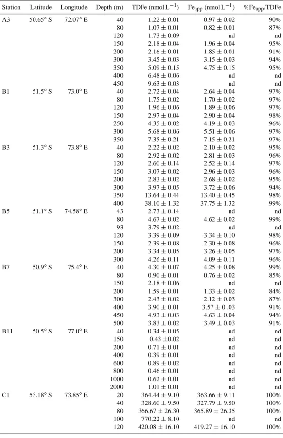
Table 1. Total dissolvable iron (TDFe), apparent particulate iron (Feapp) and location of the sampling stations. Feappis calculated using
dissolved iron (DFe) values from Blain et al. (2008). Uncertainties on the TDFe concentrations correspond to standard deviation of triplicate measurements of the sample measured 3 times. Uncertainties on the Feappcorrespond to the sum of the TDFe and DFe uncertainties. nd
represents “not determined” values.
Station Latitude Longitude Depth (m) TDFe (nmol L−1) Feapp(nmol L−1) %Feapp/TDFe
A3 50.65◦S 72.07◦E 40 1.22 ± 0.01 0.97 ± 0.02 90% 80 1.07 ± 0.01 0.82 ± 0.01 87% 120 1.73 ± 0.09 nd nd 150 2.18 ± 0.04 1.96 ± 0.04 95% 200 2.16 ± 0.01 1.85 ± 0.01 91% 300 3.45 ± 0.03 3.15 ± 0.03 94% 350 5.09 ± 0.15 4.75 ± 0.15 95% 400 6.48 ± 0.06 nd nd 450 9.63 ± 0.03 nd nd B1 51.5◦S 73.0◦E 40 2.72 ± 0.04 2.64 ± 0.04 97% 80 1.75 ± 0.02 1.70 ± 0.02 97% 120 1.96 ± 0.06 1.89 ± 0.06 97% 150 2.97 ± 0.04 2.90 ± 0.04 98% 250 4.35 ± 0.02 4.19 ± 0.03 96% 300 5.68 ± 0.06 5.51 ± 0.06 97% 350 7.35 ± 0.21 7.15 ± 0.21 97% B3 51.3◦S 73.8◦E 40 2.22 ± 0.02 2.10 ± 0.02 95% 80 2.92 ± 0.02 2.81 ± 0.03 96% 120 2.60 ± 0.14 2.52 ± 0.14 97% 150 3.07 ± 0.02 2.96 ± 0.03 96% 200 2.83 ± 0.02 2.68 ± 0.02 95% 300 3.97 ± 0.05 3.72 ± 0.06 94% 350 13.64 ± 0.44 13.40 ± 0.45 98% 400 38.10 ± 1.32 37.75 ± 1.32 99% B5 51.1◦S 74.58◦E 43 2.73 ± 0.14 nd nd 80 4.67 ± 0.02 4.62 ± 0.02 99% 93 3.79 ± 0.02 nd nd 120 3.39 ± 0.09 3.34 ± 0.10 98% 150 2.39 ± 0.08 2.30 ± 0.08 96% 200 3.34 ± 0.05 3.26 ± 0.05 97% 300 4.26 ± 0.11 4.09 ± 0.11 96% B7 50.9◦S 75.4◦E 40 4.30 ± 0.07 4.25 ± 0.08 99% 80 0.90 ± 0.01 0.76 ± 0.02 85% 150 2.18 ± 0.06 nd nd 200 1.59 ± 0.01 1.33 ± 0.02 84% 300 2.43 ± 0.02 2.12 ± 0.03 87% 400 3.90 ± 0.01 3.57 ± 0 .03 91% 450 4.93 ± 0.03 4.63 ± 0.04 94% 500 3.83 ± 0.02 3.49 ± 0.03 91% B11 50.5◦S 77.0◦E 40 0.34 ± 0.05 nd nd 150 0.43 ±0.02 nd nd 200 0.71 ± 0.01 nd nd 400 0.39 ± 0.01 nd nd 600 0.89 ± 0.02 nd nd 800 0.46 ± 0.01 nd nd 1000 0.62 ± 0.01 nd nd 2000 1.01 ± 0.01 nd nd C1 53.18◦S 73.85◦E 20 364.44 ± 9.10 363.66 ± 9.11 100% 40 328.60 ± 9.50 327.79 ± 9.50 100% 80 366.67 ± 26.30 365.89 ± 26.35 100% 100 770.22 ± 8.10 nd nd 120 420.08 ± 16.10 419.27 ± 16.10 100%
Table 1. Continued.
Station Latitude Longitude Depth (m) TDFe (nmol L−1) Feapp(nmol L−1) %Feapp/TDFe
C5 52.42◦S 75.6◦E 40 2.19 ± 0.05 2.13 ± 0.05 97% 80 5.02 ± 0.03 4.95 ± 0.03 99% 120 2.22 ± 0.03 2.14 ± 0.03 96% 150 4.10 ± 0.02 4.02 ± 0.02 98% 200 18.42 ± 3.80 18.16 ± 3.80 99% 300 17.29 ± 2.40 16.99 ± 2.40 98% 400 15.97 ± 1.50 15.60 ± 1.51 98% 450 65.59 ± 1.00 65.07 ± 1.02 99% 500 51.42 ± 8.00 50.84 ± 8.01 99% C11 51.65◦S 77.73◦E 40 0.97 ± 0.03 0.84 ± 0.03 87% 80 0.98 ± 0.01 0.91 ± 0.02 93% 120 1.00 ± 0.01 nd nd 200 0.56 ± 0.02 0.49 ± 0.02 87% 400 0.53 ± 0.01 0.47 ± 0.01 89% 500 1.74 ± 0.02 nd nd 600 2.23 ± 0.07 1.99 ± 0.07 89% 800 1.55 ± 0.01 1.28 ± 0.01 82% 1000 2.02 ± 0.01 1.76 ± 0.01 87%
Table 2. Range of total dissolvable iron (TDFe), apparent particulate iron (Feapp) and percentage of Feappin the total dissolvable fraction
in the water column for different seasons and sectors of the Southern Ocean ((a) Sarthou et al., 1997, (b) L¨oscher et al., 1997, (c) Sedwick et al., 1997, (d) Sedwick et al., 2008), for a coastal environment in the Pacific Ocean ((e) Chase et al., 2005, (f) Johnson et al., 2001, (g) Fitzwater et al., 2003) and for the Atlantic Ocean ((h) Croot et al., 2004).
[Fe] (nmol L−1) on Total dissolvable Apparent particulate % the whole water column Location Iron (nmol L−1) Iron (nmol L−1) (Feapp/TDFe)
Open Ocean Indian Sector, summer (this study) 0.34–2.23 0.47–1.99 83–93 (mean: 86 ± 3) Indian Sector, summer (a) 0.6–4.8
Atlantic Sector, spring (b) 0.5–8.9 0–6.86 0–97 Australian Sector, summer (c) 0.17–1.3 0.02–1.07 0-81 Fe rich waters Indian Sector, summer (this study) 0.9–65.6 0.8–65.1 82–99 (mean: 95 ± 5)
Indian Sector, summer (a) 6.2 Australian Sector, spring (d) 12.5 Monterey Bay, California, summer (e) 0.3–17.4
Monterey Bay, California, spring (f) 25 ∼80 Monterey Bay, California (g) 0.80–6.57
Equatorial Atlantic (h) 0.3–6 0–5 0–80 (mean: 46 ± 12)
source (Sedwick et al., 2008). Concentrations higher than 10 nmol L−1 and 25 nmol L−1 were reported by Chase et
al. (2005) and Johnson et al. (2001) respectively, in the up-welling system of Monterey Bay, California. The higher val-ues determined by L¨oscher et al. (1997) in the Atlantic sector of the Southern Ocean are explained by the upwelling of iron rich Antarctic waters
Apparent particulate iron (Feapp) concentrations,
calcu-lated by subtracting DFe values measured during the cruise (Blain et al., 2008) from TDFe, are reported in Table 1. Feapp
is defined as the iron adsorbed on lithogenic or biogenic
par-ticles, the biogenic iron and the labile lithogenic particulate iron (de Baar et al., 1999) plus the refractory colloids in-cluded in the dissolved fraction and that were not measured on board after a few days of acid storage. Feapprepresents
be-tween 82 and 99% of the TDFe (mean value 95±5%) above the plateau and between 83 and 93% (mean value 86±3%) outside the plateau with no difference between surface and deep water (see Table 1). This suggests that particles or re-fractory colloids largely dominated the iron pool. Such high percentages were previously observed in the open ocean and in enriched waters but with a larger variability. L¨oscher et
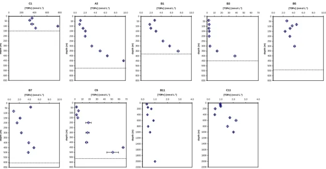
C1 0 50 100 150 200 250 300 350 400 450 500 550 600 650 0 200 400 600 800 [TDFe] (nm ol L-1) d e p th ( m ) A3 0 50 100 150 200 250 300 350 400 450 500 550 600 650 0.0 2.0 4.0 6.0 8.0 10.0 [TDFe] (nm ol L-1) d e p th ( m ) B1 0 50 100 150 200 250 300 350 400 450 500 550 600 650 0.0 2.0 4.0 6.0 8.0 10.0 [TDFe] (nm ol L-1) d e p th ( m ) B3 0 50 100 150 200 250 300 350 400 450 500 550 600 650 0 10 20 30 40 50 60 70 [TDFe] (nm ol L-1) d e p th ( m ) B5 0 50 100 150 200 250 300 350 400 450 500 550 600 650 0.0 2.0 4.0 6.0 8.0 10.0 [TDFe] (nm ol L-1) d e p th ( m ) B7 0 50 100 150 200 250 300 350 400 450 500 550 600 650 0.0 2.0 4.0 6.0 8.0 10.0 [TDFe] (nm ol L-1) d e p th ( m ) C5 0 50 100 150 200 250 300 350 400 450 500 550 600 650 0 10 20 30 40 50 60 70 [TDFe] (nm ol L-1) d e p th ( m ) B11 0 200 400 600 800 1000 1200 1400 1600 1800 2000 2200 0.0 1.0 2.0 3.0 4.0 [TDFe] (nm ol L-1) d e p th ( m ) C11 0 200 400 600 800 1000 1200 1400 1600 1800 2000 2200 0.0 1.0 2.0 3.0 4.0 [TDFe] (nm ol L-1) d e p th ( m )
Fig. 2. Vertical profiles of total dissolvable iron (TDFe, nmol L−1) at C1 station (near Heard Island), above the plateau (A3, B1, B3, B5, B7
and C5) and outside the plateau (B11 and C11). Depicted are mean values ±1 SD. Depth and concentration scales are not the same for all the stations. For stations located above the plateau, the dashed lines represent the bottom depth.
al. (1997), Sedwick et al. (1997) and Croot et al. (2004) ob-served percentages of Feappvarying between 0 and more than
80% in the Atlantic sector of the Southern Ocean, the Aus-tralian sector of the Southern Ocean and the Equatorial sector of the Atlantic Ocean, respectively (Table 2).
4 Discussion
The onboard study of the concentration of DFe above the plateau highlighted the existence of a deep dissolved iron-rich reservoir below the mixed layer (Blain et al., 2007). The main sources of DFe in the surface waters were identified to be diapycnal diffusive mixing and the utilisation of the win-ter stock (Blain et al., 2008), but a comparison of iron supply versus iron demand of phytoplankton suggested that an ad-ditional iron source was present, and that was possibly the dissolution of lithogenic particles (Blain et al. 2007, 2008; Sarthou et al., 2008). Additionally, the study of the rare-earth elements (REE) showed that Heard Island could be a significant source of lithogenic material in the water column above the plateau (Zhang et al., 2008). This source is also evidenced by elevated228Ra activities above the plateau (van Beek et al., 2008). The lateral advection of water masses that have been in contact with the continental shelf of Heard Is-land should thus be considered as a possible source of partic-ulate and dissolved iron above the plateau. In the following section, we focus on the Feapp and the DFe fractions. The
different sources of particulate and dissolved iron above the plateau are investigated and a budget of iron is presented.
The main objectives of this budget were to better define the geochemical cycle of Fe during the KEOPS cruise, and no-tably to explore the role of the TDFe as a tracer of lithogenic inputs coming from Heard Island, a mechanisms shown for other tracers (REE,228Ra. . . ) (van Beek et al., 2008; Zhang et al., 2008) but not for Fe yet. It was also used to refine the C sequestration efficiency. The question of the bioavailability of these particles is also discussed.
4.1 Budget of iron above the Kerguelen plateau 4.1.1 Description of the model
A two box-model including pools and fluxes of dissolved and particulate iron was used to determine an iron budget above the Kerguelen plateau. A steady state was assumed to al-low the construction of this budget. Results of the calculated fluxes will give information on the relevance of this assump-tion. The model is illustrated in Fig. 3a. The area covered by these boxes is the surface plateau (i.e. 45 000 km2). The
surface box represents the upper 150 m of the water column. This depth stratum was chosen in accordance with the study of Blain et al. (2008) who observed a higher vertical gradi-ent of DFe below 150 m for the stations located above the plateau. The deep box represents the depth stratum 150 m – bottom depth, with increasing depth from the incoming (325 m depth) to the exit (500 m depth) of the box in accor-dance with the topography of the plateau (Park et al., 2008a). All the sources and sinks of dissolved and particulate iron in the two boxes are listed below with the corresponding
inflowing and outflowing fluxes. The sedimentary source which could play a significant role is taken into account for the dissolved pool but data are lacking for the particulate flux calculation. Finally, the isopycnal mixing is neglected. In-deed, Maraldi et al. (2009) studied the influence of the short term (∼ less than a week) lateral mixing on the phytoplank-ton bloom over the Kerguelen Plateau. They concluded that the spatial pattern of the bloom was delimited by a barrier of high lateral mixing due essentially to tides, with minor con-tributions from Ekman transport, geostrophy or barotropic at-mospheric forced currents. Mongin et al. (2008) also showed that the effect of lateral diffusion has little effect on the over-all carbon and iron budgets. We have therefore decided to make the same assumptions for our iron budget model.
The four following equations are used to describe the vari-ation with time of dissolved and particulate iron in surface and deep waters.
d[DFe]1
dt ·V 1 = Ad·S + (Fw1· [DFe]C)1+DMd + WSd (1)
−Fw1· [DFe]plateau1−E1
d[DFe]2
dt ·V 2 = (Fw1· [DFe]C)2+(Fw2· [DFe]C)2 (2)
+Sedd−DMd − WSd − Fw2· [DFe]plateau2−E2
d[Feapp]1 dt ·V 1 = Ap·S+(Fw1· [Feapp]C)1+DMp+E1 (3) −Fw1· [Feapp]plateau1−F1 d[Feapp]2 dt ·V 2 = (Fw1· [Feapp]C)2+(Fw2· [Feapp]C)2 (4) +E2 + F1 − DMp − Fw2· [Feapp]plateau2−F2
Numbers 1 and 2 correspond to the surface and the deep layer respectively. “V ” and “S” represent the box volume and the box surface. Letters “d” and “p” refer to the dissolved and the particulate fluxes. “A” represents the atmospheric in-puts. “Fw” represents the water flux. “Plateau” represents the mean concentration above the plateau and “C” represents the mean concentration along transect C. “DM” represents the inflowing flux in the surface layer coming from the di-apycnal mixing, “WS” refers to the winter stock. “E” cor-responds to the net fluxes exchanged between dissolved and particulate fraction. “F” refers to the particle fluxes at the bottom of each box.
To estimate lateral inflowing and outflowing fluxes of iron in our model, we used the mean current velocity estimated by Park et al. (2008b) above the plateau (4.0±0.5 cm s−1).
The corresponding hydrological fluxes (Fw) are calculated by multiplying this current by the section of the box (350 km width and 150 m depth for the upper box, 350 km width and 175 m and 350 m depth for the entrance and the exit of the deep box, respectively). These water fluxes are multiplied by the mean dissolved or particulate iron concentrations along
the transect C or above the plateau, in the upper or deep boxes. These mean concentrations are reported in Table 3. We assumed that the water flux transporting dissolved and apparent particulate iron from the transit C in the surface box is uniform over the 500 m water column leading to the two different fluxes (Fw1·[DFe]C)1 and (Fw1·[DFe]C)2 for the
DFe, and (Fw1·[Feapp]C)1and (Fw1·[Feapp]C)2for the Feapp
fraction (Fig. 3a). Figure 3b displays the results of the calcu-lated stocks and fluxes.
4.1.2 Budget calculation Atmospheric inputs
One of the main external sources of iron to the surface wa-ters of the open ocean is aeolian dust deposition (Jickells et al., 2005). During the cruise, aerosols were collected to estimate atmospheric fluxes to the Southern Ocean, and in particular iron fluxes over the study area (Wagener et al., 2008). A total iron flux (dry + wet) of 23±9 nmol m−2d−1 was estimated. Assuming a solubility ranging from 1 to 10% (Bonnet and Guieu, 2004; Baker and Jickells, 2006), the atmospheric dissolved iron flux over the Kerguelen plateau can be estimated to be 0.2–3.2 nmol m−2d−1 (Wagener et al., 2008). A mean value of 1.7±2.1 nmol m−2d−1 is con-sidered hereafter. These fluxes are low compared to those calculated during the Crozex and FeCycle cruises, which were 100 nmol m−2d−1(Planquette et al., 2007) and 7.58– 75.8 nmol m−2d−1, respectively, assuming a 1–10% dis-solution of the total flux given by Boyd et al. (2005). The particulate iron flux (90–99% of the total flux) during KEOPS was estimated to be 12.6–31.7 nmol m−2d−1 with
a mean value of 22.2±13.5 nmol m−2d−1. Over an area of 45 000 km2, the atmospheric fluxes Ad · S and Ap · S equal 76.5±94.5 mol d−1 and 999±607 mol d−1for the dissolved and particulate iron, respectively. Given that the other partic-ulate fluxes calcpartic-ulated in our budget represent apparent par-ticulate fluxes, this atmospheric flux may be overestimation. Diapycnal diffusive fluxes
The enrichment of DFe and Feapp for the stations located
above the plateau (see Fig. 2) clearly indicates an input of iron from the bottom of the water column. Park et al. (2008b) estimate a vertical eddy diffusivity (Kz) of 3.8±2.4×10⁻⁴m2s−1 in the seasonal pycnocline (80 m<
z <180 m) at A3 using a Thorpe scale analysis. By
multiply-ing this coefficient by the vertical gradient of Feappcalculated
at this station (8.6 nmol m−4 between 80 and 200 m), a di-apycnal mixing of 283±178 nmol m−2d−1can be estimated. Above the plateau, Kz was only estimated at A3 station. As-suming that the diapycnal mixing is homogeneous over all the plateau area, we calculate a flux of particles (DMp) of 12 735±8010 mol d1. The vertical supply calculated for DFe at A3 is 31 nmol m−2d−1(Blain et al., 2008). With the same
Table 3. Mean dissolved and apparent particulate iron concentrations calculated above and below 150 m, for all the stations located above
the plateau and for the stations located along transect C.
Upper box Deep box
Feapp(nmol L−1) DFe (nmol L−1) Feapp(nmol L−1) DFe (nmol L−1)
Transect C∗ 186±39 0.44±0.03 33.74±23.17 0.41±0.14 Above the plateau 2.43±1.04 0.09±0.03 6.66±8.13 0.23±0.08
∗Values in the upper box correspond to the mean of the two stations C1 and C5. Values in the deep box correspond to the mean of the single
station C5.
assumption that this mixing is homogeneous, we calculate a dissolved flux (DMd) of 1395 mol d−1.
Winter mixing
The second mechanism of fertilization mentioned by Blain et al. (2007, 2008) for dissolved iron is the utilisation of the winter stock above the plateau. During winter, the strong winds allow a greater mixing of the surface waters. The thickness of the mixed layer can reach 200 m. As deep wa-ter contains higher concentration of iron than surface wawa-ter (Blain et al., 2008), at the beginning of the spring, surface water is enriched in iron. This stock is called winter stock. To calculate the stock of iron potentially available for phyto-plankton growth, the thermal structure of the water column has to be known. The temperature minimum is indicative of the winter concentration (Cwinter). The mean concentration
of DFe measured within the mixed layer is called the sum-mer concentration (Csummer). The winter stock utilization
(nmol m−2d−1) is calculated using the following equation
(Cwinter-Csummer)·MLD/90 where MLD represents the mean
mixed layer depth (70 m at A3) and 90 days is the duration of the bloom. Winter stock utilization was 52 nmol m−2d−1for the DFe (Blain et al., 2008). Assuming that this flux is ho-mogeneous over all the surface of the plateau, we calculate a winter mixing flux (WSd) of 2340 mol d−1for the dissolved iron.
Lateral advection
Lateral advection is a potential source of dissolved and par-ticulate iron above the plateau. Apart from some sporadic mesoscale intrusions (Zhang et al., 2008), the circulation above the KEOPS study area rules out any transport of waters from the Kerguelen Island to the plateau (Park et al., 2008a), whereas a lateral advection from the south can be considered. General mean circulation above the plateau is described in Fig. 1. Waters that have interacted with the continental shelf of Heard Island can be transported onto the plateau. This source is also recognised for other tracers like 228Ra (van Beek et al., 2008), lithogenic Ba (Jacquet el al., 2008) and rare-earth elements (Zhang et al., 2008).
Using the mean current velocity estimated by Park et al. (2008b) above the plateau in the 500 m water column, the hydrological fluxes (Fw) are calculated by multiplying this current by the section of the box, leading to a surface water flux of 1.81±0.23×10¹⁴L d−1. For the deep box, values of 2.12±0.26×10¹⁴L d−1for the inflowing flux and 4.23±0.53×10¹⁴L d−1 for the outflowing flux are calcu-lated. In the surface box, multiplying the water flux by the DFe concentrations from the transect C, (Fw1×[DFe]C)1
and (Fw1·[DFe]C)2 give values of 23.9±4.6×10³mol d−1
and 55.9±10.8×10³mol d−1, respectively. Con-cerning the Feapp fraction, (Fw1·[Feapp]C)1 and
(Fw1·[Feapp]C)2 give values of 10 138±3396×103mol d−1
and 23 656±7923×103mol d−1, respectively. In the deep
box, (Fw2·[DFe]C)2 and (Fw2·[Feapp]C)2 give flux values
of 85.9±40.4 and 7142±5797×103mol d−1, respectively
(Fig. 3b).
Sedimentary inputs
Over the plateau, inputs of DFe in the water column from the sediment were measured during the cruise and com-prised of a flux of 136 µmol m−2d−1 (Blain et al., 2008), higher than previous fluxes calculated along the Californian coast (Elrod et al., 2004). This equates to a flux Sedd of
6120×103mol d−1, assuming it is homogeneous over the plateau.
4.1.3 Dissolved and particulate budgets
Results are reported in Fig. 3b. Atmospheric deposi-tion is a negligible source of Feapp above the plateau,
as already observed for DFe (Blain et al., 2008). Lat-eral advection is the predominant source of iron above the plateau, for Feapp but also for DFe (although the
un-certainty in the calculation of this flux is important). A Tukey test with different “n” values (from 3 to 50) shows that the lateral advection is always statistically different from the atmospheric and diapycnal fluxes (p < 0.001) for DFe and Feapp. The corresponding fluxes are equal
to 9697±3640×103mol d−1 (=10 138–441×103mol d−1)
and 8.3±11.6×10³mol d−1 (=23.9–15.6×10³mol d−1) for
WSd (Fw2*[DFe]C)2 (Fw2*[Feapp]C)2 175 m 350 m DMd DMp Fw2*[DFe]plateau2 Fw2*[Feapp]plateau2 Fw1*[DFe]plateau1 Fw1*[Feapp]plateau1 (Fw1*[DFe]C)1 (Fw1*[Feapp]C)1 (Fw1*[DFe]C)2 (Fw1*[Feapp]C)2
[DFe]plateau1 ---> [Feapp]plateau1
[DFe]plateau2 ---> [Feapp]plateau2
E1 E2 Ad*S Ap*S F1 F2 150 m DFe stock 1 Feapp stock 1 DFe stock 2 Feapp stock 2 Sedd
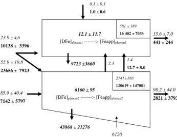
Fig. 3a. Dissolved and particulate iron 2-box budgets above the
Kerguelen Plateau. Numbers 1 and 2 correspond to the surface and the deep layer, respectively. “V ” and “S” represent the box volume and the box surface. Letters “d” and “p” refer to the dissolved and the particulate fluxes. “A” represents the atmospheric inputs. “Fw” represents the water flux. “Plateau” represents the mean concentra-tion above the plateau and “C” represents the mean concentraconcentra-tion along transect C. “DM” represents the inflowing flux in the surface layer coming from the diapycnal mixing, “WS” refers to the winter stock. “E” corresponds to the net fluxes exchanged between dis-solved and particulate fraction. “F” refers to the particle fluxes at the bottom of each box. We consider a surface layer of 150 m and a deep layer below 150 m with increasing depth from the transect C to the plateau. Dissolved iron fluxes are represented with num-bers in italic. Particulate iron fluxes are represented with numnum-bers in bold. Numbers in bold and italic are calculated from the reso-lution of the 4 equations describing the variation of dissolved and particulate iron with time.
of the total net fluxes of Feappand DFe that enter the surface
box, respectively.
The biogenic pool of Fe of 80±9 pmol L−1calculated by Sarthou et al. (2008) represents 540×103mol in our surface box (150 m depth, area of 45 000 km2). It is only 3.3% of
the apparent particulate iron stock calculated in our surface box (16 402×103mol, see Fig. 3b), which suggests that the biogenic fraction is not predominant. Whatever the state of the bloom, this result confirms a posteriori our assumption of a steady state.
At steady-state, left members of the Eqs. (1–4) are equal to 0. Values of E1, E2, F1 and F2 can be calculated by resolv-ing these 4 equations and are reported in Fig. 3b. Values of 12.1±11.7×10³and 6160±95×103mol d−1were calculated respectively for E1 and E2.
The positive values of E1 and E2 suggest a predomi-nant transport of iron from the dissolved to the apparent particulate fraction. Processes involved in such a transport are biological uptake, colloidal aggregation, adsorption on phytoplankton cells and scavenging by non-living particles (through adsorption, precipitation or aggregation), whereas
2.3 85.9 ± 40.4 7142 ± 5797 9723 ±3660 43868 ± 21276 1.4 12.7 ± 8.0 98.2 ± 44.0 2821 ± 3793 15.6 ± 7.0 441 ± 244
[DFe]plateau1 ---> [Feapp]plateau1
[DFe]plateau2 ---> [Feapp]plateau2
12.1 ± 11.7 6160 ± 95 0.1 ± 0.1 1.0 ± 0.6 581 ± 189 16 402 ± 7033 2741± 885 120619 ± 147081 6120 23.9 ± 4.6 10138 ± 3396 55.9 ± 10.8 23656 ± 7923
Fig. 3b. Numerical values of dissolved (in italic) and
particu-late (in bold) iron fluxes (in 103mol d−1) and stocks (in 103mol). Stocks are obtained by multiplying the mean concentrations cal-culated above the plateau in Fig. 3a by the volume of the boxes (6.75×10¹²m3for the surface box and 1.81×10¹³m3for the deep box).
processes responsible for the transfer of apparent particulate iron to the dissolved iron pool are due to the dissolution and regeneration of particulate or colloidal iron (Sarthou and Je-andel, 2001).
Using the radiotracer55Fe, the phytoplankton net Fe de-mand in the bloom (uptake minus regeneration) was equal to 208±77 nmol m−2d−1 (Sarthou et al., 2008). Adsorp-tion on phytoplankton cells and scavenging by non-living particles represented between 20 and 37% of the total genic iron (Sarthou et al., 2008), leading to a total bio-genic iron flux of 260–330 nmol m−2d−1. Assuming an area of 45 000 km2, this gives a flux varying between 11.7×10³ and 14.9×10³mol d−1. These values are close to E1 (12.1±11.7×10³mol d−1), suggesting that the dissolution of
Feappmay not be significant.
Taking into account the maximum value of the flux cal-culated from the 55Fe experiment (14.9×10³mol d−1)
and the minimum value of the E1 flux (ie 12.1– 11.7=0.4×10³mol d−1), a maximum dissolution of 14.5×10³mol d−1 can however be estimated. As the biogenic pool represents 3.3% of the total pool (see above), the maximum dissolution of lithogenic material is esti-mated to 14.0×10³mol d−1. It represents 0.14% of the total apparent particulate flux that enters in the upper box (10 138×103mol d−1). If we assume that all the DFe at
C1 comes from the dissolution of Feapp, a dissolution of
0.2% is calculated. These values are in the same range as those calculated by Bonnet and Guieu (2004) and listed by Jickells et al. (2001) for the dissolution of lithogenic Fe from atmospheric dusts.
The exchange flux between the dissolved and apparent particulate fraction in deep waters (E2) also shows a posi-tive value, two orders of magnitude higher than in surface waters. This suggests that scavenging and/or aggregation are predominant in the deep waters. This could be due to the high transport of particulate material in the deep box and to the inputs from the sediments.
Values of 9723±3660×103 and 43 868±21 276×103 mol d−1were calculated for the particulate sinking fluxes F1 and F2, respectively. This budget suggests that most of the particles that flow above the plateau are removed from the water column by sedimentation.
The calculation of F1 allows us to estimate the res-idence time (RT) of apparent particulate iron (RT=PFe stock/downward PFe flux, Boyd et al., 2005). It is equal to 1.7 days in surface waters. This value is lower than that of 100 days estimated during the FeCycle experiment (Boyd et al., 2005). Residence times varying between 6 (range 2-12 days) and 62 (range 21–186) days for total iron (dis-solved + particulate) were calculated in the Equatorial sector of the Atlantic Ocean (Croot et al., 2004). The shortest res-idence times were associated with high particulate Fe flux. In our budget, the high supply of Feappfrom the weathering
of Heard Island, which is rapidly removed by sinking, may explain the very low residence times calculated. It should be noted here that such a dynamic system could have implica-tion for the scavenging of dissolved iron which could thus be overestimated in the surface box of our budget. Additionally, such a short residence time could lead to an underestimation of the apparent particulate iron concentration. Indeed, dur-ing the time required for particulate sampldur-ing, large particles (>20 µm) could have sunk below the level of the spigots on the Go-Flo bottles which would affect the apparent particu-late iron concentration (Gardner et al., 2003).
Considering a mean dissolved iron stock in the up-per 150 m of the water column above the plateau of 581×103mol, and a supply of DFe of 12.1×10³mol d1 (=(Ad ·S+DMd+WSd+HSd), with HSd equal to the
horizontal supply of iron above the plateau (=(23.9– 15.6)×103mol d−1)), we estimated a DFe residence time
equal to 48 days. Such a value is consistent with residence times of ∼10 days–1 year observed in the North and Equa-torial Atlantic Ocean (Jickells, 1999; de Baar and de Jong, 2001; Sarthou et al., 2003, 2007).
4.2 Importance of the colloidal fraction to the bioavailability of Fe
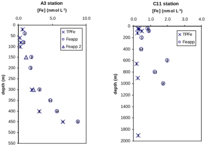
Vertical profiles of total and apparent particulate iron at sta-tions A3 and C11 are plotted in Fig. 4. For both stasta-tions, higher values are observed in the Feapppool compared to the
TPFe pool. Indeed, Feappconcentrations are 1.3 to 3.1 times
higher than TPFe. Given that some very refractory particu-late Fe remains unreactive to the TDFe handling and analy-sis (Powell et al., 1995), Feappfraction should exhibit smaller
C11 station 0 200 400 600 800 1000 1200 1400 1600 1800 2000 0.0 1.0 2.0 3.0 4.0 [Fe] (nm ol L-1) d e p th ( m ) TPFe Feapp A3 station 0 50 100 150 200 250 300 350 400 450 500 550 0.0 5.0 10.0 [Fe] (nm ol L-1) d e p th ( m ) TPFe Feapp Feapp 2
Fig. 4. Vertical profiles of total particulate (crosses) and apparent
particulate iron (cercles) iron at A3 (left) and C11 (right) stations. Depicted are mean values ±1 SD. The two triangles represented at station A3 correspond to the Feapp concentrations calculated with
the dissolved samples measured at the shore-based laboratory, 18 months after sampling (Feapp2) (see text for more details).
concentrations than TPFe. Several reasons might explain this difference. First, for the 2 stations TPFe was sampled 10 days before TDFe and DFe. Given that the residence time of iron particles is 1.7 days, changes in the transport of particles could have occurred during this period. Second, an incom-plete digestion of particulate material, leading to an underes-timation of the TPFe values might have occurred, since the digestion protocol did not include a strong attack with HF acid. Finally, another possibility would be that a substantial fraction of colloidal iron was not analysed on board in the DFe pool, but was reactive to the more acidic attack and to the time storage of the TDFe samples.
A significant fraction of dissolved iron is actually thought to be in the colloidal pool (Kuma et al., 1998; Wu et al., 2001; Cullen et al., 2006). Wu et al. (2001) and Cullen et al. (2006) observed that 80–90% of the dissolved iron is present under colloidal fraction in the surface waters and 70% in the deep waters in the Atlantic Ocean.
A few duplicates of DFe samples were stored at room tem-perature and were analysed at the same time as the TDFe samples at the laboratory (i.e. 18 months later). DFe con-centrations increased by 37–90% during these 18 months of storage. This result implies that a substantial fraction of DFe is colloidal and is only released during long acid storage. This observation confirms the work of Zhang et al. (2008) who suggest that a large pool of DFe is probably colloidal. However Feappstill dominates the total dissolvable pool after
18 months of storage. Indeed, Feapprepresents between 54
and 99% of the TDFe (mean value 85±11%, n = 27) when considering the dissolved iron samples analysed at the labo-ratory.
Only two duplicates of DFe were stored at A3 and it was possible to re-calculate the concentrations of Feapp by using
the values of DFe measured at the laboratory and to compare them with the TPFe concentrations. The new estimations of these Feappconcentrations are presented on Fig. 4 and seem
to explain the difference between the two pools. This result suggests that a significant portion of refractory colloids is present in the DFe fraction and that only a long acid storage (18 months) allows measuring this fraction.
Assuming that the colloids came from the dissolution of particulate lithogenic Fe at C1 and that the mean current velocity above the plateau is 4.0±0.5 cm s−1 (Park et al., 2008b), it takes nearly three months for the colloids to reach A3. Chen and Wang (2001) showed that freshly precipitated colloids were available to phytoplankton but aging processes (15 days) markedly reduced their availability.
Moreover, the E1 flux calculated in our budget in the sur-face box is consistent with the uptake by phytoplankton es-timated by Sarthou et al. (2008). These calculations seem to indicate that the refractory colloidal iron present in an appar-ent particulate fraction is not taken up by phytoplankton.
These results give some information on the measurements of the physical speciation of iron. First, the most labile frac-tion of DFe measured after few hours of acidificafrac-tion could be the fraction that is bioavailable to the phytoplankton. Sec-ond, more than a few days of acidification are needed to mea-sure the total dissolved iron fraction, especially in a region with high input of refractory iron. Our study indicates that 18 months of acid storage allow the measurement of the re-fractory colloids and determine the total particulate Fe from TDFe and DFe analyses. However, it should be noted that only digestion including HF acid (which was not used here) ensures the recovery of the most refractory and crystalline particles determined in the TPFe fraction. These observa-tions are in agreement with the study of Bowie et al. (2004) who considered it useful to extend the storage of acidified samples to determine the total dissolved iron pool.
4.3 Carbon sequestration efficiency
Carbon sequestration efficiency is based on the ratio of the excess of carbon exported to the dissolved iron supplied (de Baar et al., 2005). An iron supply of 5×10⁻³nmol m−2, cor-responding to the vertical supply and the winter stock uti-lization, has already been calculated by Blain et al. (2007). Taking into account the lateral advection which sup-plies 8.3×10³mol Fe d−1(=(23.9–15.6)×103mol d−1) over
an area of 45 000 km2 during 90 days, the contribution of the lateral supply can be estimated to be equal to 16.6×10⁻³nmol m−2leading to a new estimate of dissolved iron supply of 21.6×10⁻³nmol m−2. This value is proba-bly overestimated because of a possible impact of this lateral advection on the stations located outside the bloom (C11 sta-tion for example), which would lead to a smaller excess of iron. Using the excess of particulate organic carbon (POC)
calculated by Blain et al. (2007) of 3317 nmol m−2, the new
estimated sequestration efficiency is equal to 154 000 mol C (mol Fe)−1. With our assumptions, consideration of the
lat-eral advection reduces the first estimate of the sequestra-tion efficiency by 4-fold. However, this value is still ap-poximatively 18-fold higher than the value calculated dur-ing the other study of a natural iron fertilisation experiment CROZEX (8640 mol C (mol Fe)−1, Pollard et al., 2009) and is also higher than the two artificial iron fertilisation exper-iments SOFeX (3300 mol C (mol Fe)−1, Buesseler et al., 2004) and SERIES (∼500 mol C (mol Fe)−1, Boyd et al., 2004). Blain et al. (2007) explained the higher carbon se-questration efficiency calculated during KEOPS than during SOFeX and SERIES by two reasons. First, it is suspected that the end of the bloom was reached during KEOPS but not during SOFeX, leading to a higher excess of carbon dur-ing KEOPS. Secondly, durdur-ing mesoscale enrichment experi-ments a large amount of the DFe added to seawater is rapidly loss contrary to the natural iron enrichment where the input of iron is slow and continuous (Blain et al., 2007). The com-parison of the carbon sequestration efficiency between the CROZEX and the KEOPS experiments is difficult because of the different methods used during the two studies to calculate iron supply and carbon export. However, Pollard et al. (2009) observed that during KEOPS, the supply of iron was 8-fold lower and the carbon exported was 10-fold higher than dur-ing CROZEX. They suggested that either a vertical mixdur-ing or a more intense lateral advection of lithogenic material could have occurred but before the late-summer observation period of KEOPS. Our study allowed us to better constrain the lat-eral fluxes of Fe over the plateau. Considering these fluxes, the sequestration efficiency previously calculated by blain et al. (2007) decreases, but still remains largely higher than dur-ing CROZEX. Takdur-ing into account the lateral supply, the sup-ply of iron was only 2-fold lower during KEOPS than during CROZEX. Therefore most of the difference results from dif-ferences in the excess of carbon export. Base on the data set available during both experiments it is impossible to say if this difference is real or if it results from the different ap-proaches used. In fact when the excess of carbon export at 100 m are compared the factor of difference between KEOPS and CROZEX is only 5. The extrapolation at 200 m produces an additional factor 2.
5 Conclusions
Our results suggest that TDFe in our study area predomi-nantly consists of particles. This study also highlights the im-portance of the refractory colloidal fraction in the dissolved pool and emphasises the importance of extended storage to better constrain the physical speciation of Fe. The most labile fraction of DFe measured after a few days of acidification could be the fraction that is bioavailable to the phytoplank-ton. The total particulate Fe may be determined from TDFe
and DFe analyses with sufficient acid storage (18 months). The study of the TDFe fraction above the Kerguelen Plateau gives information on iron sources, the physical speciation and the bioavailability of iron.
Our Fe budget also shows that the predominant source of Feappand DFe above the Kerguelen Plateau is the lateral
ad-vection of waters that have been in contact with the continen-tal shelf of Heard Island. It represents 99% and 69% of the total apparent particulate and dissolved iron supply, respec-tively.
By taking into account the lateral advection of dissolved iron, we calculate a revised seasonal carbon sequestration efficiency of 154 000 mol C (mol Fe)−1, 4 times lower than the one previously calculated by Blain et al. (2007), but still 18-fold higher than the one calculated during the natural iron fertilisation experiment CROZEX (Pollard et al., 2009). This result is also significantly higher than the carbon sequestra-tion efficiencies obtained during artificial iron fertilisasequestra-tion experiments. Two reasons may explain these differences: first, if Fe is supplied in a continuous way or not, second if the bloom reached its maximum or not.
This discussion points out the need for a more accurate determination of both terms of the Fe/C ratio. All the calcu-lations and discussion on the efficiency ratio are based on the assumption that DFe represents the bioavailable form of iron, and clearly this assumption impacts heavily on the Fe/C data and calculations of carbon sequestration efficiencies. The numbers and the conclusions might dramatically change if we discover in the future that this hypothesis is falsified.
Acknowledgements. We are grateful to the project coordinator
St´ephane Blain, to Bernard Qu´eguiner, the chief scientist, and to the captain and crew of the R. V. Marion Dufresne for their support on board. We also acknowledge Thibaut Wagener for his help with sampling clean seawater. This work was supported by the Institut National des Sciences de l’Univers (INSU) and the French Polar Institute (Institut Polaire Emile Victor, IPEV). This research was partly supported by the Australian Government Cooperative Research Centres Program through the Antarctic Climate and Ecosystems CRC (ACE CRC) and the French-Australian Science and Technoloy (FAST) programme (contract number FR040170). We thank ACE CRC internal reviewers Brian Griffiths and Del-phine Lannuzel for their comments. P. Boyd and an anonymous reviewer are gratefully acknowledged for their critical comments and suggestions.
Edited by: D. Turner
The publication of this article is financed by CNRS-INSU.
References
Baker, A. R., Jickells, T. D., Witt, M., and Linge K. L.: Trends in the solubility of iron, aluminium, manganese and phosphorus in aerosol collected over the Atlantic Ocean, Mar. Chem., 98, 43– 58, 2006.
Blain, S., Qu´eguiner, B., Armand, L., Belviso, S., Bombled, B., Bopp, L., Bowie, A. R., Brunet, C., Brussaard, C., Carlotti, F., Christaki, U., Corbi`ere, A., Durand, I., Ebersbach, F., Fuda, J. L., Garcia, N., Gerringa, L., Griffiths, B., Guigue, C., Guillerm, C., Jacquet, S., Jeandel, C., Laan, P., Lef`evre, D., Lo Monaco, C., Malits, A., Mosseri, J., Obernesterer, I., Park, Y. H., Picheral, M., Pondaven, P., Remenyi, T., Sandroni, V., Sarthou, G., Savoye, N., Scoarnec, L., Souhaut, M., Thuiller, D., Timmermans, K., Trull, T., Uitz, J., van Beek, P., Veldhuis, M., Vincent, D., Viollier, E., Vong, L., and Wagener, T.: Effect of natural iron fertilization on carbon sequestration in the Southern Ocean, Nature, 446, 7139, 1070–1074, 2007.
Blain, S., Sarthou, G., and Laan, P.: Distribution of dissolved iron during the natural iron-fertilization experiment KEOPS (Kergue-len Plateau, Southern Ocean), Deep Sea Res. II, 55(5–7), 594– 605, 2008.
Bonnet, S. and Guieu C.: Dissolution of atmospheric iron in seawater, Geophys. Res. Lett., 31(3), L03303, doi:10.1029/2003GL018423, 2004.
Bowie, A. R., Sedwick, P. N., and Worsfold, P. J.: Analyti-cal intercomparison between flow injection–chemiluminescence and flow injection–spectrophotometry for the determination of picomolar concentrations of iron in seawater, Limnol. Oceanogr. Methods, 2, 42–54, 2004.
Boyd, P. W., Watson, A. J., Law, C. S., Abraham, E. R., Trull, T., Murdoch, R., Bakker, D. C. E., Bowie, A., Buesseler, K. O., Chang, H., Charette, M., Croot, P., Downing, K., Frew, R., Gall, M., Hadfield, M., Hall, J., Harvey, M., Jameson, G., LaRoche, J., Liddicoat, M., Ling, R., Maldonado, M. T., McKay, R. M., Nodder, S., Pickmere, S., Pridmore, R., Rintoul, S., Safi, K., Sut-ton, P., Strzepek, R., Tanneberger, K., Turner, S., Waite, A., and Zeldis, J.: A mesoscale phytoplankton bloom in the polar South-ern Ocean stimulated by iron fertilization, Nature, 407, 695–702, 2000.
Boyd, P. W., Law, C. S., Wong, C. S., Nojiri, Y., Tsuda, A., lev-asseur, M., Takeda, S., Rivkin, R., Harrison, P. J., Strzepek, R., Gower, J., McKay, R. M., Abraham, E., Arychuk, M., Barwell, C. J., Crawford, W., Crawford, D., Hale, M., Harada, K., John-son, K., Kiyosawa, H., Kudo, I., Marchetti, A., Miller, W., Nee-doba, J., Nishioka, J., Ogawa, H., Page, J., Robert, M., Saito, H., Sastri, A., Sherry, N., Soutar, T., Sutherland, N., Taira, Y., Whit-ney, F., Wong, S. K. E., and Yoshimura, T.: The decline and fate of an iron-induced subarctic phytoplankton bloom, Nature, 428, 549–553, 2004.
Boyd, P. W., Law, C. S., Hutchins, D. A., Abraham, E. R., Croot, P. L., Ellwood, M., Frew, R. D., Hadfield, M., Hall, J., Handy, S., Hare, C. E., Higgins, J., Hill, P., Hunter, K. A., Leblanc, K., Maldonado, M. T., Mckay, R. M., Mioni, C., Oliver, M., Pickmere, S., Pinkerton, M., Safi, K., Sander, S., Sanudo-Wilhelmy, S. A., Smith, M., Strzepek, R., Tavor-Sanchez, A., and Wilhelm S. W.: FeCycle: Attempting an iron biogeochem-ical budget from a mesoscale SF6 tracer experiment in unper-turbed low iron waters, Global Biogeochem. Cy., 19, GB4S20, doi:10.1029/2005GB002494, 2005.
Bruland, K. W. and Rue, E. L.: Analytical Methods for the De-termination of Concentrations and Speciation of Iron, Biogeo-chemistry of Fe in Seawater, D.R. Turner and K.A. Hunter, SCOR/IUPAC series, J Wiley, Chapter 6, 255–290, 2001. Buesseler, K. O., Andrews, J. E., Pike, S. M., and Charette, M. A.:
The effects of iron fertilization on carbon sequestration in the Southern Ocean, Science, 304, 5669, 414–417, 2004.
Chase, Z., Johnson, K. S., Elrod, V. A., Plant, J. N., Fitzwater, S. E., Pickella, L., and Sakamoto, C. M.: Manganese and iron distri-butions off central California influenced by upwelling and shelf width, Mar. Chem., 95, 235–254, 2005.
Chen, M. and Wang, W.-X.: Bioavailability of natural colloid-bound iron to marine plankton: Influences of colloidal size and aging, Limnol. Oceanogr., 46(8), 1956–1967, 2001.
Coale, K. H., Johnson, K. S., Chavez, F. P., Buesseler, K. O., Bar-ber, R. T., Brzezinski, M. A., Cochlan, W. P., Millero, F. J., Falkowski, P. G., Bauer, J. E., Wanninkhof, R. H., Kudela, R. M., Altabet, M. A., Hales, B. E., Takahashi, T., Landry, M. R., Bidi-gare, R. R., Wang, X. J., Chase, Z., Strutton, P. G., Friederich, G. E., Gorbunov, M. Y., Lance, V. P., Hilting, A. K., Hiscock, M. R., Demarest, M., Hiscock, W. T., Sullivan, K. F., Tanner, S. J., Gordon, R. M., Hunter, C. N., Elrod, V. A., Fitzwater, S. E., Jones, J. L., Tozzi, S., Koblizek, M., Roberts, A. E., Herndon, J., Brewster, J., Ladizinski, N., Smith, G., Cooper, D., Timothy, D., Brown, S. L., Selph, K. E., Sheridan, C. C., Twining, B. S., and Johnson, Z. I.: Southern ocean iron enrichment experiment: Carbon cycling in high- and low-Si waters, Science, 304, 5669, 408–414, 2004.
Croot, P. L., Streu, P., and Baker, A. R.: Short residence time for iron in surface seawater impacted by atmospheric dry deposi-tion from Saharan dust events, Geophys. Res. Lett, 31, L23S08, doi:10.1029/2004GL020153, 2004.
Cullen, J. T. and Sherrell, R. M.: Techniques for determination of trace metals in small samples of size-fractionated particulate matter: phytoplankton metals off central California, Mar. Chem., 67(3–4), 233–247, 1999.
Cullen, J. T., Bergquist, B. A., and Moffett, J. W.: Thermodynamic characterization of the partitioning of iron between soluble and colloidal species in the Atlantic Ocean, Mar. Chem., 98, 295– 303, 2006.
de Baar, H. J. W., de Jong, J. T. M., Nolting, R. F., Timmermans, K. R., van Leeuwe, M. A., Bathmann, U., van der Loeff, M. R., and Sildam, J.: Low dissolved Fe and the absence of diatom blooms in remote Pacific waters of the Southern Ocean, Mar. Chem., 66, 1–34, 1999.
de Baar, H. J. W. and de Jong, J. T. M.: Distributions, Sources and Sinks of Iron in Seawater, Biogeochemistry of Fe in Seawater, D. R. Turner and Hunter, K. A., Baltimore, SCOR-IUPAC series, J Wiley, Chapter 5, 123–253, 2001.
de Baar, H. J. W., Boyd, P. W., Coale, K. H., and Tsuda, A.: Synthe-sis of eight in situ iron fertilizations in high nutrient low chloro-phyll waters confirms the control by wind mixed layer depth of phytoplankton blooms, J. Geophys. Res., 110, 700–724, 2005. Elrod, V. A., Berelson, W. M., Coale, K. H., and Johnson, K.
S.: The flux of iron from continental shelf sediments: A miss-ing source for global budgets, Geophys. Res. Lett., 31, L12307, doi:10.1029/2004GL020216, 2004.
Fitzwater, S. E., Johnson, K. S., Elrod, V. A., Ryana, J. P., Colettia, L. J., Tanner, S. J., Gordon, R. M., and Chavez, F. P.: Iron,
nu-trient and phytoplankton biomass relationships in upwelled wa-ters of the California coastal system, Cont. Shelf Res., 23, 1523– 1544, 2003.
Frew, R. D., Hutchins, D. A., Nodder, S., Sanudo-Wilhelmy, S., Tovar-Sanchez, A., Leblanc, K., Hare, C. E., and Boyd, P. W.: Particulate iron dynamics during FeCycle in subantarctic wa-ters southeast of New Zealand, Global Biogeochem. Cy., 20, GB1S93, doi:10.1029/2005GB002558, 2006.
Gardner, W. D., Richardson, M. J., Carlson, C. A., Hansell, D., and Mishonov, A. V.: Determining true particulate organic carbon: bottles, pumps and methodologies, Deep Sea Res. II, 50(3–4), 655–674, doi:10.1016/S0967-0645(02)00589-1, 2003.
Jacquet, S. H. M., Dehairs, F., Savoye, N., Obernosterer, I., Chris-taki, U., Monnin, C., and Cardinal, C.: Mesopelagic organic carbon remineralization in the Kerguelen Plateau region tracked by biogenic particulate Ba, Deep Sea Res. II, 55(5–7), 868–879, 2008.
Jickells, T.: The inputs of dust derived elements to the Sargasso Sea: a synthesis, Mar. Chem., 68, 5–14, 1999.
Jickells, T. and Spokes, L. J.: Atmospheric iron inputs to the oceans. The biogeochemistry of Iron in seawater, edited by: Turner, D. R. and Hunter, K. A., Baltimore, SCOR-IUPAC series, J Wiley, Chapter 4, 85–121, 2001.
Jickells, T. D., An, Z. S., Andersen, K. K., Baker, A. R., Bergametti, G., Brooks, N., Cao, J. J., Boyd, P. W., Duce, R. A., Hunter, K. A., Kawahata, H., Kubilay, N., La Roche, J., Liss, P. S., Ma-howald, N., Prospero, J. M., Ridgwell, A. J., Tegen, I., and Tor-res, R.: Global Iron Connections Between Desert Dust, Ocean Biogeochemistry, and Climate, Science, 308, 67–71, 2005. Johnson, K. S., Chavez, F. P., Elrod, V. A., Fitzwater, S. E.,
Pin-nington, J. T., Buck, K. R., and Walz, P. M.: The annual cycle of iron and the biological response in central California coastal waters, Geophys. Res. Lett., 28(7), 1247–1250, 2001.
Johnson, K. S., Boyle, E., Bruland, K., Coale, K., Measures, C., and Moffett, J.: Sampling and Analysis of Fe: The SAFE Iron Inter-comparison Cruise, Eos Trans. AGU, 87, 36, Ocean Sci. Meet. Suppl., Abstract OS11N-02, 2006.
Johnson, K. S., Boyle, E., Bruland, K., Coale, K., Measures, C., and Moffett, J.: Developing Standards for Dissolved Iron in Seawa-ter, Eos Trans. AGU, 88(11), 131–132, 2007.
Kuma, K., Katsumoto, A., Nishioka, J., and Matsunaga, K.: Size-fractionnated iron concentrations and Fe(III) hydroxide solubil-ities in various coastal waters, Estuarine, Coast. Shelf Sci., 47, 275–283, 1998.
Kutska, A. B., Carpenter, E. J., and Sanudo-Wilhelmy, S. A.: Iron and marine nitrogen fixation: progress and future directions, Res. Microbiol., 153, 255–262, 2002.
Lannuzel, D., Remenyi, T., Lam, P., Townsend, A., Ibisanmi, E., Butler, E., Wagener, T., Schoemann, V., and Bowie, A. R.,: Dis-tribution of dissolved and particulate iron in the sub-Antarctic and Polar Frontal Southern Ocean (Australian sector), Deep Sea Res. II, accepted, 2010.
L¨oscher, B. M., de Baar, H. J. W., de Jong, J. T. M., Veth, C., and Dehairs, F.: The distribution of Fe in the Antarctic Circumpo-lar Current. Ecology and biogeochemistry of the Antarctic Cir-cumpolar Current during austral spring: Southern Ocean JGOFS cruise ANT X/6 of R.V. Polarstern, Deep Sea Res. II, 44(1–2), 143–187, 1997.
organically bound iron by Thalassiosira oceanica (Bacillario-phyceae), J. Phycol, 37(2), 298–309, 2001.
Maraldi, C., Mongin, M., Coleman, R., and Testut, L.: The influ-ence of lateral mixing on a phytoplankton bloom: Distribution in the Kerguelen Plateau region, Deep Sea Res. I., 56(6), 963–973, 2009.
Mongin, M., Molina, E., and Trull, T. W.: Seasonality and scale of the Kerguelen plateau phytoplankton bloom: A remote sens-ing and modelsens-ing analysis of the influence of natural iron fertil-ization in the Southern Ocean, Deep Sea Res. II, 55, 880–892, 2008.
Morel, F. M. M., Kustka, A. B., and Shaked, Y.: The role of unchelated Fe in the iron nutrition of phytoplankton, Limnol. Oceanogr., 53(1), 400–404, 2008.
Obata, H., Karatani, H., and Nakayama, E.: Automated determi-nation of iron in seawater by chelating resin concentration and chemiluminescence, Anal. Chem., 65, 1524–1528, 1993. Park, Y.-H., Roquet, F., Durand, I., and Fuda, J. L.: Large-scale
cir-culation over and around the Northern Kerguelen Plateau, Deep Sea Res. II, 55(5–7), 566–581, 2008a.
Park, Y.-H., Fuda, J.-L., Durand, I., and Naveira Garabato, A. C.: Internal tides and vertical mixing over the Kerguelen Plateau, Deep Sea Res. II, 55(5–7), 582–593, 2008b.
Planquette, H., Statham, P. J., Fones; G. R., Charette, M. A., Moore, C. M., Salter, I., Nedelec, F. H., Taylor, S. L., French, M., Baker, A. R., Mahowald, N., and Jickells, T. D.: Dissolved iron in the vicinity of the Crozet Islands, Southern Ocean, Deep Sea Res. II, 54, 1999–2019, 2007.
Pollard, R. T., Salter, I., Sander, S., Lucas, M. I., Moore, C. M., Mills, R. A., Statham, P. J., Allen, J. T., Baker, A. R., Bakker, D. C. E., Charette, M. A., Fielding, S., Fones, G. R., French, M., Hickman, A. E., Holland, R. J., Hughes, J. A., Jickells, T. D., Lampitt, R. S., Morris, P. J., Nedelec, F. H., Nielsdottir, M., Planquette, H., Popova, E. E., Poulton, A. J., Read, J. F., Seeyave, S., Smith, T., Stinchcombe, M., Taylor, S. L., Thomalla, S., Ven-ables, H. J., Williamson, R., and Zubkov, M.: Southern Ocean deep-water carbon export enhanced by natural iron fertilization, Nature, 457, 577–581, 2009.
Powell, R. T., King, D. W., and Landing, W. M: Iron distributions in the surface waters of the south Atlantic, Mar. Chem., 50(1–4), 13–20, 1995.
Rueter, J. G. and Ades, D. R.: The role of iron nutrition in photo-synthesis and nitrogen assimilation in Scenedesmus quadeicauda (Chlorophyceae), J. Physicol., 23, 452–457, 1987.
Sarthou, G., Jeandel, C., Brisset, L., Amouroux, D., and Donard, O. F. X.: Fe and H2O2distributions in the upper 250 meters of the
water column in the Indian sector of the Southern Ocean, Earth Planet. Sci. Lett., 147, 83–92, 1997.
Sarthou, G. and Jeandel, C.: Seasonal variations of iron concentra-tions in the Ligurian Sea and iron budget in the Western Mediter-ranean Sea, Mar. Chem., 74(2–3), 115–129, 2001.
Sarthou, G., Baker, A. R., Blain, S., Achterberg, E. P., Boye, M., Bowie, A. R., Croot, P. L., Laan, P., de Baar, H. J. W., Jick-ells, T. D., and Worsfold, P. J.: Atmospheric iron deposition and sea-surface dissolved iron concentrations in the eastern Atlantic Ocean, Deep Sea Res. I, 50(10–11), 1339–1352, 2003.
Sarthou, G., Baker, A. R., Kramer, J., Laan, P., La¨es, A., Ussher, S., Achterberg, E. P., de Baar, H. J. W., Timmermans, K. R., and Blain, S.: Influence of atmospheric inputs on the iron distribution in the subtropical North-East Atlantic Ocean, Mar. Chem., 104, 186–202, 2007.
Sarthou, G., Vincent, D., Christaki, U., Obernesterer, I., Timmer-mans, K. R., and Brussaard, C. P. D.: The fate of biogenic iron during a phytoplankton bloom induced by natural fertilization: Impact of copepod grazing, Deep Sea Res. II, 55(5–7), 734–751, 2008.
Schlitzer, R.: Ocean Data View, online available at: http://odv.awi. de, 2007.
Sedwick, P. N., Edwards, P. R., Mackey, D. J., Griffiths, F. B., and Parslow, J. S.: Iron and manganese in surface waters of the Australian subantarctic region, Deep-Sea Res. I, 44, 1239–1253, 1997.
Sedwick, P. N., Bowie, A. R., and Trull, T. W.: Dissolved iron in the Australian sector of the Southern ocean (CLIVAR SR3 section): Meridional and seasonal trends, Deep Sea Res. I, 55, 911–925, 2008.
Sunda, W. G.: Trace metal interactions with marine phytoplankton, Biol. Oceanogr., 6, 411–442, 1989.
Townsend, A. T.: The accurate determination of the first row tran-sition metals in water, urine, plant, tissue and rock samples by sector field ICP-MS, J. Anal. Atom. Spec., 15, 307–314, 2000. van Beek, P., Bourquin, M., Reyss J.-L., Souhaut, M., Charrette,
M. A., and Jeandel, C.: Radium isotopes to investigate the wa-ter mass pathways on the Kerguelen Plateau (Southern Ocean), Deep Sea Res. II, 55(5–7), 622–637, 2008.
Wagener, T., Guieu, C., Losno, R., Bonnet, S., and Mahowald, N.: Revisiting atmospheric dust export to the Southern Hemisphere ocean: Biogeochemical implications, Global Biogeochem. Cy., 22, GB2006, doi:10.1029/2007GB002984, 2008.
Wu, J., Boyle, E., Sunda, W., and Wen, L.-S.: Soluble and col-loidal iron in the oligotrophic North Atlantic and North Pacific, Science, 293, 847–849, 2001.
Zhang, Y., Lacan, F., and Jeandel, C.: Dissolved rare earth elements tracing lithogenic inputs over the Kerguelen Plateau (Southern Ocean), Deep Sea Res. II, 55(5–7), 638–652, 2008.