HAL Id: hal-00329083
https://hal.archives-ouvertes.fr/hal-00329083
Submitted on 1 Jan 1998
HAL is a multi-disciplinary open access
archive for the deposit and dissemination of sci-entific research documents, whether they are pub-lished or not. The documents may come from teaching and research institutions in France or abroad, or from public or private research centers.
L’archive ouverte pluridisciplinaire HAL, est destinée au dépôt et à la diffusion de documents scientifiques de niveau recherche, publiés ou non, émanant des établissements d’enseignement et de recherche français ou étrangers, des laboratoires publics ou privés.
to estimate the mean dynamic topography of the North
Atlantic and improve the geoid
P. Legrand, H. Mercier, T. Reynaud
To cite this version:
P. Legrand, H. Mercier, T. Reynaud. Combining T/P altimetric data with hydrographic data to estimate the mean dynamic topography of the North Atlantic and improve the geoid. Annales Geo-physicae, European Geosciences Union, 1998, 16 (5), pp.638-650. �hal-00329083�
to estimate the mean dynamic topography of the North Atlantic
and improve the geoid
P. LeGrand1, H. Mercier1, and T. Reynaud1,2
1Laboratoire de Physique des OceÂans, Unite mixte CNRS-IFREMER-Universite de Bretagne Occidentale, IFREMER centre de Brest, B.P. 70, F-29280 PlouzaneÂ, France
2Now at LEG1/MEOM, Institut de MeÂcanique de Grenoble, B.P. 53, F-38041 Grenoble CEDEX, France Received: 4 July 1997 / Revised: 9 January 1998 / Accepted: 16 January 1998
Abstract. The mean dynamic topography of the surface of the North Atlantic is estimated using an inverse model of the ocean circulation constrained by hydro-graphic and altimetric observations. In the North Atlantic, altimetric observations have no signi®cant impact on the topography estimate because of the limited precision of available geoid height models. They have a signi®cant impact, however, when uncertainties in the density ®eld are increased to simulate interpolat-ion errors in reginterpolat-ions where hydrographic data are scarce. This result, which moderates the conclusion drawn by Ganachaud and co-workers of no signi®cant contribution of altimetric observations to the determi-nation of the large-scale steady circulation, re¯ects the simple idea that altimetric data are most useful near the surface of the ocean and in areas where the hydrography is poorly determined. One application of the present inverse estimate of the mean dynamic topography is to compute a geoid height correction over the North Atlantic which reduces the uncertainty in the geoid height expanded to spherical harmonic 40 down to a level of about 5 cm.
Key words. Oceanography: general (climate and interannual variability) á Oceanography: physical (general circulation; remote sensing)
1 Introduction
During the past few years, much has been learned on the variable component of the ocean circulation using the Topex/Poseidon (T/P) observations. The determination of the mean component of the circulation from altimetric measurements, however, is still hampered by
the lack of a precise estimate of the geoid height. The geoid height is the elevation the surface of the ocean would have if it were at rest, and it must be subtracted from the altimetric sea surface height to determine the dynamic topography associated with oceanic currents. The error in existing geoid height models exceeds the dynamic topography signal for spherical harmonic degrees larger than 15 (Nerem et al., 1994), and the ability of altimetric data to determine the mean circulation at spatial scales smaller than about 1000 km is therefore limited. Moreover, Ganachaud et al. (1997) ®nd that the ability of altimetric observa-tions to improve signi®cantly the large-scale circulation derived from an inversion of hydrographic data is also limited, despite the fact that the geoid height error is smaller than the topographic signal at larger scales.
The impact of altimetric observations on the deter-mination of the mean circulation is re-examined in this work using a ®nite dierence inverse model (Mercier et al., 1993) instead of the box inverse model used by Ganachaud et al. (1997). The ®nite dierence model adjusts the density ®eld, uses altimetric observations away from the location of hydrographic sections, and produces an estimate of the mean dynamic topography of the surface of the ocean over a regular grid (Le Traon and Mercier, 1992). The altimetric observations intro-duced in the model consist of an estimate of the mean dynamic topography obtained by subtracting the JGM-2 geoid height model from the mean sea surface height observed by T/P. The impact of these observations is evaluated by comparing the mean dynamic topography estimated by the model when the altimetric constraint is included to that estimated using in situ observational constraints only. Two outcomes are possible: (1) if the altimetric constraint is more precise, or as precise as the topography estimated by the inverse model using in situ observations only, then this constraint will have a signi®cant impact and will improve the inverse solution; and (2) if the altimetric constraint is far less precise, it will have no signi®cant impact on the inverse solution other than insuring that the solution is consistent with the
geodesic information contained in this constraint. In this case, the geoid height model obtained by subtracting the inverse topography estimate from the observed mean sea surface height (Roemmich and Wunsch, 1982) is likely to be more precise than existing geoid height models.
The study is divided into six sections. Following this introduction, Sect. 2 describes the direct altimetric estimate of the mean dynamic topography over the North Atlantic that will be used to constrain the inverse model. Section 3 describes a hydrographic estimate of the mean dynamic topography that illustrates the potential of in situ observations to determine the topography of the ocean. Section 4 presents an inverse estimate of the mean dynamic topography calculated by a combination of dynamical constraints and hydro-graphic data and another estimate in which altimetric data are also incorporated. In accordance with Ga-nachaud et al.'s (1997) conclusion, altimetric observa-tions are found to be fully consistent with geostrophic dynamics and hydrographic observations, but to weakly constrain the mean dynamic topography estimate in the North Atlantic. Section 5, however, shows that al-timetric data do constrain this estimate if the density ®eld is poorly known, and can provide useful informa-tion in regions like the Southern Ocean that are poorly sampled by the hydrographic data base. The impact of uncertainties in the density ®eld and the dierences between the present calculation and that of Ganachaud et al. (1997) are discussed in this section. Finally, Sect. 6 summarizes the results of this study and concludes by using the inverse model's topography estimate to calcu-late a geoid height correction in the North Atlantic. The precision of the corrected geoid height is on the order of 5 cm at spatial scales of about 500 km.
2 An altimetric estimate using T/P data and the JGM-2 geoid
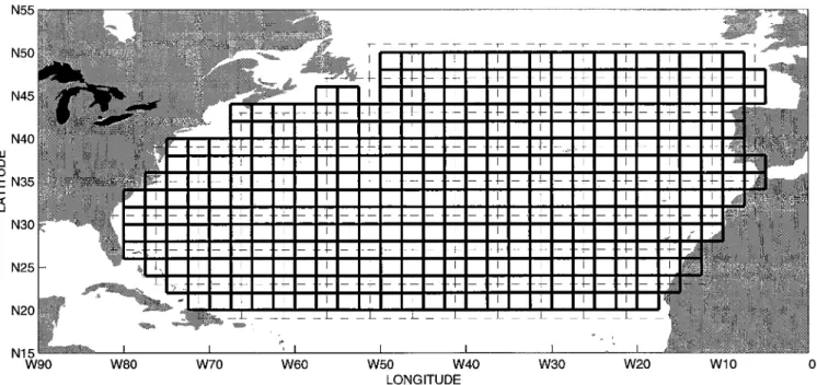
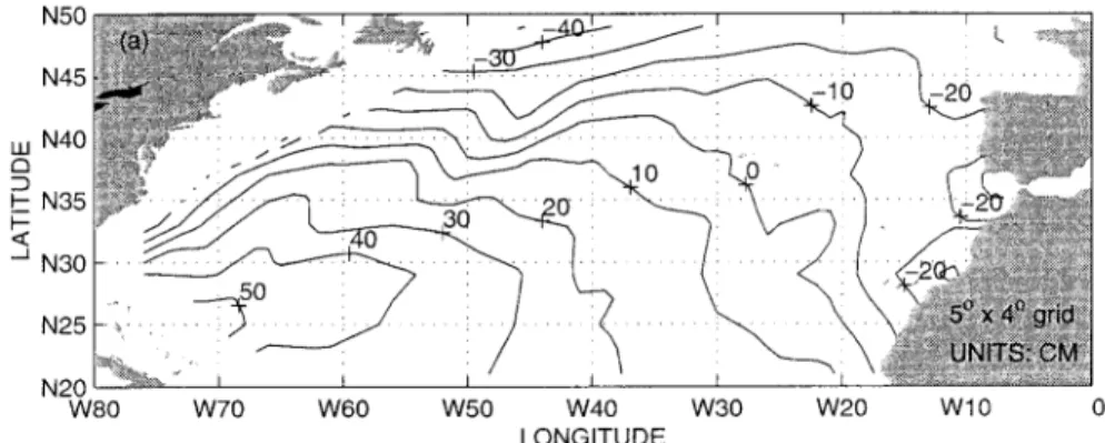
One way to estimate the mean dynamic topography of the surface of the ocean is to subtract an estimate of the geoid height from the mean sea surface height observed by an altimeter. This altimetric estimate will serve as a useful basis of comparison for other estimates and will be used to constrain the inverse calculations of Sects. 4 and 5. In this section, the geoid height computed using the JGM-2 gravimetry ®eld solution (Tapley et al., 1994) is subtracted from the mean of 2 y of T/P sea surface height observations (cycles 2 to 75). Corrections are applied to the T/P sea surface height measurements to remove the in¯uence of the troposphere (dry and wet), of oceanic waves, and of the inverse barometer eect. The dierence between the sea surface height and the geoid height yields an estimate of the mean dynamic topography along satellite tracks in the North Atlantic between 20°N and 50°N. This estimate is averaged onto a 5° longitude by 4° latitude grid (Fig. 1) to take advantage of the higher precision of the geoid model at larger scales, while approximately preserving the main features of the Gulf Stream and of the subtropical gyre (Fig. 2).
The JGM-2 geoid height uncertainty (Tapley et al., 1994) is much larger than the uncertainty in the mean sea surface height observed by T/P and is the main source of uncertainty in the altimetric estimate of the mean dynamic topography. The uncertainty in the geoid height estimate is calculated using a spatial autocorre-lation function (Rapp, Le Traon, personal communica-tion, 1994) corresponding to an expansion of the geoid to spherical harmonic 40. The error covariance of the geoid height is divided by 2 prior to the mean dynamic
Fig. 1. The solid lines represent the 2.5° longitude ´ 2° latitude density grid of the inverse model. The thin dashed lines represent the 5° longitude ´ 4° latitude grid used to compute the altimetric estimate of mean dynamic topography (Sect. 2)
topography uncertainty calculation to take into account that the geoid height error is smaller over oceans than over land (Rapp, Le Traon, personal communication, 1994), and the resulting geoid height uncertainty is about 18 cm. The uncertainty in the mean sea surface height is estimated in the 5° ´ 4° boxes using the T/P observations. The number of independent observations inside a box is determined assuming that the oceanic mesoscale variability, which is the main source of uncertainty in the mean sea surface height, has a decorrelation scale of 100 km. The resulting sea surface height uncertainty is less than 5 cm in the interior of the ocean and is about four times smaller than the geoid height uncertainty. The uncertainty in the mean dynam-ic topography calculated using the T/P sea surface height and the JGM-2 geoid is roughly uniform over the 20°N±50°N domain and is on the order of 20 cm. This uncertainty corresponds to an uncertainty in surface velocities averaged over 200 km on the order of 10 cm/s. 3 A diagnostic estimate using hydrographic data
The mean dynamic topography of the North Atlantic is diagnosed from a compilation of more than 100 000 hydrographic stations collected over the past 70 years. About 25 000 of these stations are deeper than 1000 m
(Fig. 3). Some recent data come from the Laboratoire de Physique des OceÂans compilation, but most data come from the large historic data set of the US National Oceanographic Data Center. The station density pro®les are gridded onto the inverse model 2.5° longitude ´ 2° latitude ®nite dierence grid (Fig. 1). Their variance gives an estimate of the uncertainty in the gridded density ®eld (see the Appendix).
The thermal wind equation is integrated assuming a reference level of no motion at 3000 decibars or the bottom, which ever is shallower, up to the surface to calculate surface velocities. These velocities are integrat-ed with respect to horizontal coordinates to estimate, using the geostrophic balance, the mean dynamic topography over the North Atlantic. The arbitrary integration constant is determined by the condition that the volume of the North Atlantic is ®xed in a steady state calculation. This condition sets the spatial mean of the dynamic topography over the basin, this spatial mean being determined by the T/P altimetric observa-tions for consistency with the altimetric topography estimate of the previous section.
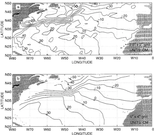
The mean dynamic topography diagnosed from hydrographic data is consistent with what is known of the ocean circulation. The mean Gulf Stream is apparent as a front a few degrees wide as well as the North Atlantic extension (Fig. 4a). Recirculation zones are
Fig. 2. Mean dynamic topography calculated on the 5° longitude ´ 4° latitude grid using T/ P observations of the mean sea surface height and the JGM-2 geoid height
Fig. 3. Distribution, after quality control, of the hydrographic stations in the data compi-lation that are deeper than 1000 m depth
present north and south of the Gulf Stream (Fig. 4a). This estimate of the mean dynamic topography is averaged (Fig. 4b) on to the 5° ´4° grid for comparison with the altimeric estimate (Fig. 2). In the hydrographic estimate (Fig. 4b), the isocontours which correspond to the Gulf Stream are almost zonal near Cape Hatteras and seem to re¯ect the separation of the Gulf Stream, whereas this separation is not apparent in the altimetric estimate (Fig. 2). The absence of Gulf Stream separation in the altimetric estimate may be caused by errors in the marine geoid height estimate. Thus, the mean dynamic topography diagnosed from the density ®eld appears to be more consistent with what is known of the ocean circulation than the mean dynamic topography estimat-ed from T/P data and the JGM-2 geoid.
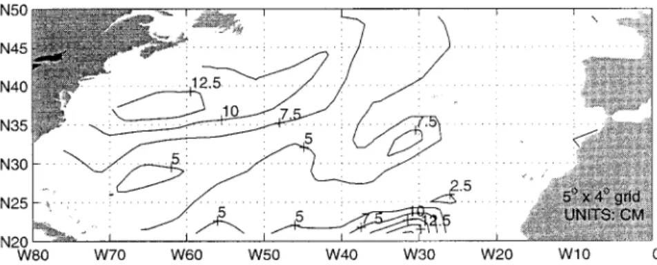
The uncertainty in the hydrographic estimate of the mean dynamic topography is diagnosed from the uncertainty in the density ®eld and the uncertainty in the reference velocities. The reference velocities are the velocities at the reference level of no motion and are assumed to be zero within reasonable uncertainties of 2 cm/s in the interior of the ocean, and 10 cm/s near the western boundary. These uncertainties contribute to less than 25% of the total topography uncertainty. The uncertainty in the topography averaged onto the 5° ´ 4° grid is less than 10 cm everywhere except near the western boundary (Fig. 5). The uncertainty is also larger than 10 cm around [30°W, 20°N], (Fig. 5) because of interpolation errors. Indeed, there are several bins in this area that do not contain enough stations to compute the mean density and its standard deviation, and these
quantities must be interpolated (Appendix). The spatial distribution of the topography uncertainty (Fig. 5) makes physical sense. It is maximum near the western boundary, where the uncertainty in the mean density ®eld is largest because of the strong mesoscale variabil-ity. Except for the small region around [30°W, 20°N], mentioned already, it is minimum in the relatively quiescent southeastern corner of the model domain. The uncertainty in the mean dynamic topography, diagnosed from the density ®eld, is consistent, both in distribution and amplitude, with the temporal variability in the dynamic height directly estimated from T/P observa-tions averaged onto a 5° longitude ´ 2° latitude grid (White and Tai, 1995). This consistency indicates that the uncertainty in the mean dynamic topography, diagnosed from the density ®eld, is mostly due to the oceanic variability. Globally, this uncertainty is smaller by a factor of 2 than the 20 cm uncertainty in the altimetric estimate of dynamic topography of section II. The mean dynamic topography estimated from hydro-graphic data is thus more precise than the one estimated from T/P and JGM-2.
4 Inverse estimates combining T/P altimetric data with hydrographic data
In this section, the mean dynamic topography of the North Atlantic is estimated using the inverse model of Mercier et al. (1993). The model ®nds an ocean circulation, and the associated dynamic topography,
Fig. 4. a Mean dynamic topography (cm) diagnosed from the density ®eld on the 2.5° longitude ´ 2° latitude grid. b Same as a but averaged onto the 5° longitude ´ 4° latitude grid
that best ®ts in a least-square sense the hydrographic and altimetric observational constraints with simpli®ed dynamical constraints relevant to the large-scale ocean circulation. The observations and the dynamics are discretized onto a 2.5° longitude by 2° latitude grid (Fig. 1). Thus, the model provides an estimate of the mean dynamic topography with a spatial resolution on the order of 200 km. The inverse model provides a realistic calculation of the uncertainty in the mean dynamic topography because it accounts for uncertain-ties in the mean density ®eld. A similar inverse calculation of the mean dynamic topography was done by Le Traon and Mercier (1992). The present calcula-tion is improved compared to their calculacalcula-tion in a number of points: (1) altimetric observations are included in the model; (2) the density ®eld is estimated from a large historic data set instead of a limited hydrographic data base; and (3) the uncertainty in the density ®eld is directly estimated from the hydrographic data and is more realistic (see the Appendix). The model is constrained by the binned density ®eld of Sect. 3 and by the altimetric topography estimate of Sect. 3. The impact of altimetric constraints on the solution uncer-tainty reduction is compared to that of the dynamical constraints in the three model runs detailed later. 4.1 Run 1. No dynamical constraints except for geostrophy In run 1, both altimetric data and hydrographic data are used as observational constraints. The density and velocity ®elds are constrained by the thermal wind relation and the mean dynamic topography by the geostrophic relation. These relations are the only dynamical constraints, mass conservation and tracer conservation are not imposed. This calculation is equivalent to combining via least-squares the mean dynamic topographies computed from altimetry in Sect. 2 and from hydrography in Sect. 3.
The data sets used to compute the two topography estimates span dierent periods of time, two years for the altimetric data set and 70 y for the hydrographic data set, and it is necessary to de®ne which period is of interest in the present study. Following Ganachaud et al. (1997), we consider that the climatological average represented by the hydrographic data base is
the reference. In this case, the uncertainty in the altimetric topography estimate must account for possible inconsistencies between the dynamic topogra-phy corresponding to an average over the ®rst two years of T/P data and that corresponding to an average over 70 y. It is not possible to estimate the dierence between the two year mean and the climatological mean from the available altimetric data base, but an upper bound on the standard deviation of the dynamic topography due to the interannual variability is given by the mean dynamic topography uncertainty estimate of Fig. 5 which re¯ects both interannual and seasonal ¯uctuations. As this upper bound is small compared to the uncertainty in the geoid height model used to compute the altimetric topography, we assume that the dierence between the two year mean and the 70 y mean is negligible compared to the geoid height uncertainty. This assumption does not result in inconsistencies in the calculations that follow, and seems to be justi®ed.
The estimated mean dynamic topography is almost identical to the hydrographic estimate of Sect. 3 (Table 1). The associated uncertainty (Fig. 6), however, is reduced compared to that of Sect. 3 (Fig. 5) by about 20% in the Gulf Stream and around [30°W, 20°N]. This result shows that in the absence of mass and tracer conservation constraints, the altimetric data have a small, but signi®cant, impact on the determination of the mean dynamic topography. This impact, however, is not signi®cant in areas of small uncertainties in the hydrographic estimate of the mean dynamic topogra-phy, i.e. in areas of small uncertainties in the density ®eld. It is signi®cant only in regions where error bars in the mean dynamic topography diagnosed from the density ®eld (Fig. 5) are comparable in magnitude to error bars in the mean dynamic topography estimated from altimetric observations (about 20 cm).
4.2 Run 2. All the dynamical constraints
In run 2, we examine whether the altimetric data and the JGM-2 geoid height estimate are consistent with the dynamics of the large-scale ocean circulation. Run 2 is constrained with the same observations as run 1, but the ocean circulation and the associated topography are
Fig. 5. Uncertainty (cm) in the 5° ´ 4° mean dynamic topography estimate of Fig. 4b
required to satisfy mass, heat, and salt conservation in addition to the thermal wind and geostrophic balances. The Ekman drift derived from the Bunker (1980) wind stress is added to the geostrophic transports in the mixed layer, which is 30 m deep in the model, to represent the direct eect of wind forcing on the circulation.
Mass conservation is imposed within a small error bar (Table 2). Indeed, the density ®eld is adjusted by the inverse model, and the only possible residuals are the mass ¯ux at the air-sea interface and the interior mixing due to the contribution of unresolved small scales (Mercier et al., 1993). These residuals are small com-pared to the advective ¯uxes of mass, and mass should be nearly exactly conserved. The potential temperature and salinity ®elds, on the other hand are not adjusted by the inverse model and they contain a signal due to the eddy variability which is not ®ltered out. This signal is not consistent with the stationary dynamics of the model, so rather large error bars (Table 2) are required in the corresponding conservation constraints. Similarly, large error bars (Table 2) are associated with the potential vorticity conservation constraint to account for discretization errors and the existence of higher order dynamics near the western boundary.
Several transport constraints are imposed: (1) there is an out¯ow from the Florida Strait of 30 1 Sv (Niiler and Richardson, 1973); (2) there is no net ¯ux of mass through the northern boundary of the model (the transport across the Bering Strait is 0.8 Sv, Coachman and Aagaard, 1988; for simplicity, the ¯ux across 50°N is taken to be 0 1 Sv in the inverse model calcula-tion). The constraint of no net ¯ux of mass is applied to
all the other zonal sections of the model to enforce the conservation of mass at large scales.
An ocean circulation consistent with the observa-tional constraints and the dynamical constraints is found by the inverse model. After inversion, over 99% of the dynamical constraints are satis®ed within one standard deviation, which is better than what one expects from a gaussian distribution. Thus, within the rather large error bar of the JGM-2 geoid height estimate, the mean dynamic topography estimated from T/P altimetric data is consistent with hydrographic data and stationary ocean dynamics. Only marginal consis-tency was obtained with GEOSAT data despite the very large uncertainties in the GEOSAT altimetric estimate (Martel and Wunsch, 1993). The consistency with T/P data within much reduced error bars compared to those of GEOSAT shows the progress made in the ®eld of altimetry and geodesy in recent years.
The two data sets are consistent even if density errors are neglected, but accounting for these errors is neces-sary to estimate the uncertainty in the mean dynamic topography. The contribution of the error bars in density to the topography uncertainty is actually four times larger than the contribution of the error bars in reference velocities. Moreover, the uncertainty in the estimated mean dynamic topography hardly changes when uncertainties in the prior estimate of the reference velocities are multiplied or dived by two, but they change signi®cantly if uncertainties in the density ®eld are modi®ed.
The estimated mean dynamic topography (Fig. 7a, b) is similar to the one obtained in the previous section
Table 1. Column 1: mean uncertainty in the various estimates of the mean dynamic topography (5° ´ 4° grid) presented in this paper. Column 2: root mean square of the dierence between the 5° ´ 4° dynamic topography estimate using the dynamical and the
altimetric constraints (run 2) and the other 5° ´ 4° dynamic topography estimates. All the dynamic topography estimates are quite similar
Mean dynamic topography
estimate Mean uncertainty (cm) Root mean square oftopography dierence (cm)
T/P-JGM-2 23.1 0.58
Diagnosed from hydrography 10.8 0.39
No dynamical constraints except
thermal wind and geostrophy (run 1) 10.5 0.35
All dynamical constraints and
altimetry (run 2) 4.8 0
All dynamical constraints but no
altimetry (run 3) 4.9 0.03
All dynamical constraints and
altimetry, gap in hydrography (run 4) 12.5 0.31
All dynamical constrains but
no altimetry, gap in hydrography (run 5) 13.0 0.31
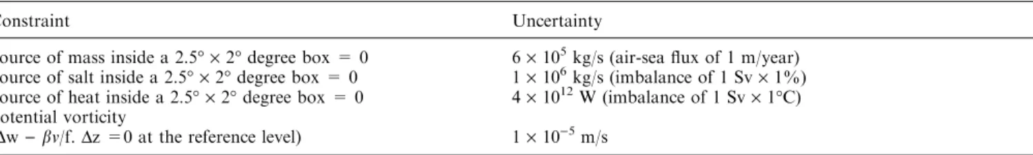
Table 2. Uncertainty in the dynamical conservation constrain imposed in the inverse model calculations
Constraint Uncertainty
Source of mass inside a 2.5° ´ 2° degree box = 0 6 ´ 105kg/s (air-sea ¯ux of 1 m/year) Source of salt inside a 2.5° ´ 2° degree box = 0 1 ´ 106kg/s (imbalance of 1 Sv ´ 1%) Source of heat inside a 2.5° ´ 2° degree box = 0 4 ´ 1012W (imbalance of 1 Sv ´ 1°C) Potential vorticity
without the conservation constraints (Table 1). The corresponding uncertainty (Fig. 8a, b), however, is much smaller, especially in the Gulf Stream area where the mean dynamic topography is poorly determined from observational constraints alone. Mass conservation and tracer conservation equally contribute to the uncertainty reduction and it is necessary to use all the conservation constraints to obtain the largest uncertainty reduction. 4.3 Run 3. All the dynamical constraints but no altimetry In run 3, we examine the contribution of the altimetric constraints to the determination of the mean dynamic topography. For that purpose, the inverse model is run
again with all the constraints of run 2 apart from the altimetric constraints. The mean dynamic topography estimated in run 3 and its uncertainty are almost identical to their counterpart in run 2 (Table 1). This result remains valid if the mean dynamic topography estimates are averaged onto a 37.5° longitude by 30° latitude grid, the altimetric constraints reducing the uncertainty in the topography at this large scale by less than 3%. Thus, the altimetric data contribute little to the solution when all the other constraints are used together. This result, consistent with that of Ganachaud et al. (1997), indicates that the present geoid height precision is too low for altimetric data to signi®cantly improve our knowledge of the mean circulation at the surface of the North Atlantic.
Fig. 6. Uncertainty (cm) in the 5° ´ 4° mean dynamic topography estimated by the inverse model combining hydrographic and altimetric observations (run 1)
Fig. 7. a Mean dynamic topography (cm) on the 2.5° ´ 2° grid estimated by the inverse model constrained by dynamical equations, hydrographic observations, and altimetric observations (run 2). b Same as a but the mean dynamic topography is averaged onto the 5° ´ 4° grid
5 Information content of altimetric data in regions where hydrographic data are scarce
It is interesting to examine whether the impact of altimetric constraints could be more signi®cant in regions of the ocean not as well sampled by the hydrographic data base as the North Atlantic. For that purpose, the inverse model is constrained with the density ®eld of the previous sections but with error bars in density multiplied by 10 in a latitude band between 30°N and 40°N. These large error bars simulate the lack of observations of the density ®eld in the large regions between hydrographic sections in calculations using a data base such as that used by Ganachaud et al. (1997). They also simulate the situation encountered in poorly sampled ocean basins such as the Southern Ocean. The natural variability of the density ®eld in this basin is dicult to estimate from the sparse hydrographic data base, but we expect it to be of the order of the variability in the Gulf Stream, i.e. ®ve times the variability in the Subtropical gyre (see the Appendix). Moreover, the density ®eld must be interpolated in the Southern Ocean over large areas void of data, even if a historic data set is used. In view of the large uncertainties introduced in the density ®eld by objective mapping procedures (e.g. Mercier et al., 1993), one can estimate the interpolation errors to double the uncertainties due to the natural variability of the ocean. Thus, the assumption that uncertainties in the density ®eld in poorly sampled and energetic regions like the Southern Ocean are one order
of magnitude larger than in the North Atlantic sub-tropical gyre is plausible.
Two model runs are performed. One run (run 4) is constrained by the density ®eld with the modi®ed error bars described, all the dynamical constraints, and the altimetric mean dynamic topography estimate of Sect. 2. The other run (run 5) is identical except that the altimetric constraint is not used. In both runs, the resulting mean dynamic topography is similar to that estimated in Sect. 4.2 (Table 1). The uncertainty in both estimates (Fig. 9a,b), however, is much larger than the uncertainty estimated in Sect. 4.2 in the 30°N±40°N latitude band because of the large uncertainties in the density ®eld in this region.
The altimetric data have a signi®cant impact on those calculations. The uncertainty in the run 4 estimate with altimetric constraint (Fig. 9a) is about 20% smaller than that in the run 5 estimate with no altimetric constraint (Fig. 9b) in the region of the subtropical gyre between 30°N and 40°N. This result shows that altimetric data do have an impact on the determination of the mean dynamic topography when the density ®eld is poorly determined.
This impact can be compared to the impact on reference-level velocity uncertainties calculated by Ga-nachaud et al. (1997). In their calculation, the uncer-tainties are reduced by less than 1.5% (variance reduced by 3%) almost everywhere when altimetric observations are used, and the maximum uncertainty reduction is 3% (variance reduced by 6%). This reduction is much smaller than the 20% topography uncertainty reduction in the present calculation.
Fig. 8. a Uncertainty (cm) in the 2.5° ´ 2° mean dynamic topography of Fig. 7a. b Uncertainty (cm) in the 5° ´ 4° mean dynam-ic topography of Fig. 7b
Two factors explain the dierence between Ga-nachaud et al.'s (1997) conclusion and the present conclusion. First, their calculation can estimate the circulation at the location of oceanic transects only, whereas the present calculation can estimate the circu-lation in regions where no hydrographic data are available. It is in these regions where the density ®eld is poorly determined that altimetric observations are most likely to provide useful constraints. A second factor is that their study estimates the impact of altimetric observations on the reference level velocities only, whereas the present work estimates the impact on surface quantities like dynamic topography. The impact of altimetric observations on deep reference velocities is smaller than the impact on surface quantities, because the presence of noise in the density ®eld introduces errors, in the integration of the thermal wind relation, that prevent the altimetric information from being transmitted to the deep ocean. This point appears clearly in the present calculation: run 4 shows a 20% reduction of the uncertainty in the mean dynamic topography compared to run 5, but no signi®cant reduction of the uncertainty in the deep reference level velocities. Thus, the dierence between the conclusion of the present calculation and that of Ganachaud et al. (1997) is explained by the dierent contexts in which the impact estimates are made and the use of dierent ®gures of merit.
In this study, we have deliberately chosen to analyze the results of the various calculations in terms of mean dynamic topography because this quantity is a variable
of the inverse model and its uncertainty can be easily calculated. Moreover, it is a dynamical quantity that is directly linked to geostrophic velocities at the surface of the ocean. This quantity is therefore representative of the circulation in the upper ocean, although it is not clear what depth range it reliably represents. Volume transports can easily be computed from the results of the various inverse calculations but their use to quantify the impact of altimetric observations requires uncertainty estimates. Transport uncertainties are unfortunately dicult to determine because they necessitate the calculation of the full covariance matrix of the density ®eld, and the appropriate software is not available yet for the Mercier et al. (1993) model. (The transport uncertainties produced by Paillet and Mercier (1997) neglect correlations in the density ®eld, and are not appropriate for the present study.) All that can be said in the present study is that transports in the upper 100 m of the ocean in run 4 and run 5 dier by a few percent, but it is not possible to tell whether these dierences are signi®cant in the absence of transport uncertainty estimates.
Ganachaud et al. (1997) estimate the impact of altimetry on oceanic transports but their calculation, based on the impact on the reference velocities, applies to transports over the whole water column and leaves out the impact on transports in the upper ocean that are more likely to be aected by altimetric constraints. Their transport uncertainty calculation neglects the contribu-tion of the uncertainty in relative velocities (Macdonald, 1995), which is likely to dominate in the upper ocean. It
Fig. 9a,b. Uncertainty (cm) in the mean dynamic topography estimated by the inverse model when error bars in the density ®eld are multiplied by 10 in the 30°N±40°N latitude band. a With altimetric constraints (run 4); b without altimetric constraints (run 5)
is not clear how their model, which does not treat density as an explicit variable, could account for this contribution.
6 Summary and discussion
The mean dynamic topography calculated by subtract-ing the JGM-2 geoid height from the T/P mean sea surface height is consistent with a data base of historical hydrographic stations and the dynamics of the large-scale ocean circulation. We ®nd, in accordance with Ganachaud et al.'s (1997) results, that this topography estimate only weakly constraints an inverse estimate of the mean ocean circulation in the North Atlantic. However, altimetric observations signi®cantly constrain the surface circulation when uncertainties in the density ®eld are increased to represent regions of the ocean where the hydrography is poorly determined. This result moderates the conclusion of no signi®cant impact of the altimetric data drawn by Ganachaud et al. (1997) from a calculation at the location of hydrographic sections and based on deep reference level velocities only.
Depending on the area considered, the uncertainty in the inverse modeling estimate of the mean dynamic topography (Fig. 8b) is between ®ve and ten times smaller than that in the altimetric estimate using the JGM-2 geoid (about 20 cm). Therefore, by subtracting the inverse topography estimate from the T/P mean sea surface height one can expect to obtain a geoid height estimate that is signi®cantly improved compared to existing models. As an illustration of this point, a
correction to the JGM-2 geoid height is estimated from the results of the inverse calculation of Sect. 4.2 (run 2). This correction is on the order of 10 cm for the geoid height estimated on the 5° longitude by 4° latitude grid (Fig. 10a). It is larger near continental margins which makes physical sense (Fig. 10a). The dierence between the inverse and the JGM-2 geoid height estimates decreases with increasing scales (Fig. 11) and is within the JGM-2 height uncertainty (Nerem et al., 1994, see their Fig. 6). At small scales, the dierence between the recent EGM-96 (Lemoine et al., 1997) height estimates and the corrected estimate is slightly smaller than the dierence between the JGM-2 estimate and the correct-ed estimate (Fig. 11). This result is encouraging because departures from the JGM-2 estimate are penalized in the inverse calculation whereas no information is given to the model about the EGM-96 estimate. It is consistent with the idea of the corrected estimate being the best available estimate of the geoid height at small scales, followed by the EGM-96 estimate, the JGM-2 estimate being the least accurate. At spatial scales larger than about 5° degrees, the inverse estimate is less consistent with the EGM-96 estimate than with the JGM-2 estimate which suggests that the correction is an improvement at small scales only. However, because the EGM-96 and the JGM-2 geoid height estimates are both quite uncertain, their use to test the corrected estimate is not conclusive and it is necessary to calculate the uncertainty in the corrected geoid height.
This uncertainty (Fig. 10b) depends on the uncer-tainty in the mean dynamic topography calculated by the inverse procedure which takes into account
model-Fig. 10. a Correction to the geoid height (cm) estimated on the 5° ´ 4° grid by the inverse model (run 2). b Uncertainty (cm) in the 5° ´ 4° corrected geoid height estimate
ling errors and observational errors. Modelling errors (Table 2) have been dicult to estimate, but their precise determination is not critical. The dierence between the topography uncertainty in a variant of run 2 with modelling errors multiplied by two and the uncertainty in a variant of run 2 with modelling errors divided by two is on the order of 1 cm in the Gulf Stream, and less than 1 cm elsewhere. Observational errors are estimated directly from the data, and they are plausible despite the crude approximations made in their calculation. The uncertainty in the density ®eld is carefully estimated in the present calculation (Appen-dix). The uncertainty in the T/P sea surface height is calculated directly from altimetric observations and, for the sake of simplicity, is assumed to be decorrelated from that of the mean dynamic topography estimated by the inverse model (the assumption of no correlation would be rigorous if the topography estimated in run 3 were used instead of that estimated in run 2). All the sources of uncertainty in the geoid height estimate have thus been accounted for in this calculation, and the result should be reliable.
The total geoid height uncertainty is on the order of 5 cm in the interior of the ocean at the scale of the 5° ´ 4° grid, and is about one third of the corresponding uncertainty in the JGM-2 estimate. The uncertainties are higher near the continents because the sea surface height is not precisely known there, the number of independent altimetric observations being small in the boxes that intersect the continents.
The 5 cm precision is as good as that expected from intermediate gravimetry missions (Minster, personal communication, 1996). Only the GOCE mission would provide a higher precision, of the order of the centimeter (Minster, personal communication, 1996), but it will take several years before such a mission can be launched. The main diculty to overcome in order to
improvement of mean circulation estimates in the upper ocean, and an inverse modelling combination of these constraints with hydrographic and dynamical con-straints will still be useful.
Acknowledgements. The inverse calculations presented in this work were carried out on the IFREMER CONVEX computer. We are grateful to R. Rapp for providing the spatial autocorrelation function of the JGM-2 geoid and to P.-Y. Le Traon for providing the mean dynamic topography calculated using the T/P observa-tions and the JGM-2 geoid. Discussions with G. Larnicol and J.-F. Minster helped us with the interpretation of the inverse calcula-tions. We thank C. Wunsch and two anonymous reviewers for their useful comments on the draft version of this paper. Tim Boyer made the National Oceanographic Data Center hydrographic data available to us and we acknowledge his assistance in compiling the data base used in this study. C. Maillard and M. Fichaut also helped with the preparation of the hydrographic data base. This work was supported in part by the French Programme National d'Etude de la Dynamique du Climat.
Topical Editor D. J. Webb thanks V. Zlotnicki and P. Challenor for their help in evaluating this paper.
Appendix: processing of the hydrographic data base The hydrographic stations compiled for this study are too numerous (over 100 000 stations) to be directly used in the inverse calculation. The hydrographic data are therefore processed to produce a climatology of the mean density ®eld over the model ®nite dierence grid (Fig. 1). The various steps of this data reduction are similar to those used in Reynaud (1996) in the context of an atlas of the entire Atlantic and are summarized here. The ®rst step in the data processing consists in projecting the salinity and temperature pro®les associ-ated with each hydrographic station onto the 35 vertical levels of the inverse model (Mercier et al., 1993). In practice, high resolution CTD stations are decimated, whereas low resolution bottle stations are interpolated using a cubic spline interpolator. The procedure is designed so that shallow stations are not extrapolated to deep levels of the ocean. Stations that do not satisfy the following quality requirements are rejected: salinity and temperature values inside a reasonable range, no local potential density inversion, no anomalous salinity or temperature peaks (Reynaud, 1996). These quality checks validate about 75% of the stations. Density is then calculated from the validated salinity and temper-ature ®elds at each standard level.
The second step consists in gridding the density pro®les by averaging them inside 2.5° longitude ´ 2° latitude boxes centred on the inverse model density grid (Fig. 1). This procedure, which is simpler than the averaging inside radii of in¯uence done by Reynaud
Fig. 11. Root mean square dierence as a function of scale between the inverse model geoid height estimate and: the JGM-2 estimate (solid line); the EGM-96 estimate (dot-dashed line)
(1996), is possible here because the boxes are quite large and the data coverage in the North Atlantic is such that several stations are available in most boxes. The mean density and its standard deviation are computed in boxes that contain at least four validated stations. As a ®nal validation test, density values that are further than three standard deviations away from the mean are discarded, and the mean is recomputed. The values corresponding to the few 2.5° longitude ´ 2° latitude boxes that contain less than four validated data points are ¯agged. At this stage, we have a set of climatological density values on the inverse model grid that we call the hh binned density ®eld ii.
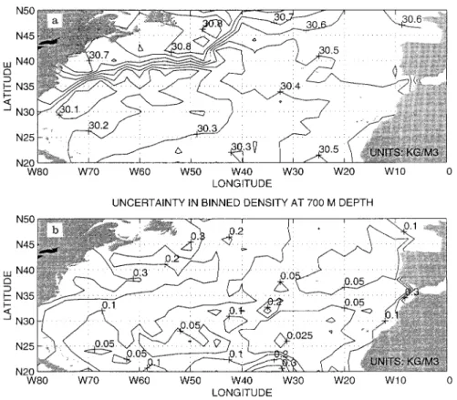
The third step to reduce the volume of data used in the inverse model is a vertical empirical orthogonal function (EOF) decomposition of the binned density ®eld. In practice, 10 modes are sucient to represent over 90% of the variance in this ®eld, and the EOF decomposition reduces the number of variables by a factor of three. The density ®eld at 700 m depth is reconstructed (Fig. 12a) using the ®rst ten EOFs. Despite the coarse resolution, the reconstructed density ®eld exhibits a Gulf Stream front that is much sharper than that of the Levitus et al. (1994) atlas.
Carefully estimating the uncertainty in the density ®eld, and thus the uncertainty in the EOF coecients, is critical for the accuracy of the inverse calculations. Several approaches are available for that purpose, and it is not obvious which one is best. The objective mapping approach used by Mercier et al. (1993) and Le Traon and Mercier (1992) has the advantage of being easy to implement, but it shows a tendency to underestimate the
uncertainty. This point is evidenced by the small uncertainties in surface velocities diagnosed from the objectively mapped EOF coecients. These uncertain-ties are on the order of a few cm/s in the Gulf Stream area2(Mercier et al., 1993), which is unrealistically small
for an unstable jet like the Gulf Stream. (In Mercier et al. (1993), uncertainties in the density ®eld, and uncertain-ties in velociuncertain-ties diagnosed from the density ®eld, are high in the northeastern Atlantic. These high uncertain-ties correspond to regions that are poorly covered by the hydrographic data base used in their study, and they are solely due to interpolation errors.) The underestimation of the uncertainties in the EOF coecients is due to the smoothing of the data introduced by the objective mapping procedure that tends to ®lter out most of the mesoscale variability. This underestimation is most obvious near sharp density fronts such as the Gulf Stream because the eect of smoothing is large there.
A dierent approach is used in the present work to estimate the uncertainty in the EOF coecients, asso-ciated with the binned density ®eld at the each grid point of the model. Inside each 2.5° ´ 2° box de®ned by the model grid, all the vertical pro®les of density corre-sponding to validated stations are projected onto the eigen vectors of the EOF decomposition of the binned density ®eld. This projection produces a local estimate of the EOF coecients at each station. It is then straightforward to compute the standard deviation of these local coecients inside the 2.5° ´ 2° boxes to estimate the uncertainty in the binned coecients. The magnitude of the uncertainty in the binned EOF coecients depends on the size of the bin used in the
Fig. 12. a Density ®eld (kg.m)3) binned onto the 2.5° longitude ´ 2° latitude grid at 700 m depth. b Uncertainty (kg.m)3) in the binned density ®eld at 700 m depth
attempted here because of the computational load required for the treatment of more than 100 000 hydrographic stations. Thus we assume that there is no correlation between the EOF coecients of distinct bins. The plausibility of the map of uncertainty in the density-diagnosed mean dynamic topography (Fig. 5) indicates that this assumption does not result in major inconsistencies with what is known of the circulation in the North Atlantic. Moreover, the density ®eld is used to constrain the inverse model, and the model introduces large-scale correlations into this ®eld through the mass and tracer conservation equations.
As a ®nal step, the binned EOF coecients and the associated uncertainties are interpolated over the few 2.5° ´ 2° boxes that do not contain enough validated data points to compute meaningful estimates of the mean and of the standard deviation (a minimum of four data points is required). The interpolated uncertainty is then subjectively multiplied by two to account for interpolation errors.
The uncertainty in the density ®eld at 700 m depth reconstructed from the ®rst ten EOFs (Fig. 12b) is much larger than that obtained by Mercier et al. (1993). It is about ®ve times larger in the Western Atlantic than in the Eastern Atlantic, which is consistent with the idea that the mesoscale activity is more intense near sharp fronts like the Gulf Stream. This realistic uncertainty yields the plausible estimates of the uncertainty in the mean dynamic topography presented here.
References
Bunker, A. F., Trends of variables and energy ¯uxes over the Atlantic Ocean from 1948 to 1972, Mon. Weather Rev., 108, 720±732, 1980.
NESDIS, vol. 3: salinity, and vol 4: temperature, National Oceanographic Data Center, 1994.
Le Traon, P.-Y., and H. Mercier, Estimating the North Atlantic mean surface topography by inversion of hydrographic and lagrangian data, Oceanol. Acta, 15, 563±566, 1992.
Macdonald, A., Oceanic ¯uxes of mass, heat and freshwater: a global estimate and perspective, Ph.D. Thesis, Department of Earth, Atmospheric, and Planetary Sciences, Massachusetts Institute of Technology, Cambridge, MA, 1995.
Martel, F., and C. Wunsch, Combined inversion of hydrography, current meter data and altimetric elevations for the North Atlantic circulation, Manuscr. Geod., 18, 219±226, 1993. Mercier, H., M. Ollitrault, and P.-Y. Le Traon, An inverse model
of the North Atlantic general circulation using Lagrangian ¯oat data, J. Phys. Oceanogr., 23, 689±715, 1993.
Nerem, R. S., F. J. Lerch, J. A. Marshall, E. C. Pavlis, B. H. Putney, B. D. Tapley, R. J. Eanes, J. C. Ries, B. E. Schutz, C. K. Shum, M. M. Watkins, S. M. Klosko, J. C. Chan, S. B. Luthcke, G. B. Patel, N. K. Pavlis, R. G. Williamson, R. H. Rapp, R. Biancale, and F. Nouel, Gravity model development for TOPEX/POSEIDON: joint gravity models 1 and 2, J. Geophys. Res., 99, 24 421±24 447, 1994.
Niiler, P. P., and W. S. Richardson, Seasonal variability of the Florida Current, J. Mar. Res., 31, 144±167, 1973.
Paillet, J., and H. Mercier, An inverse model of the eastern North Atlantic general circulation and thermocline ventilation, Deep-Sea Res. I, 44, 1293±1328, 1997.
Reynaud, T., ModeÂlisation inverse de l'Atlantique - Partie 1: Traitement des donneÂes hydrographiques, Technical Report of the Laboratoire de Physique des OceÂans, Brest, 1996.
Roemmich, D., and C. Wunsch, On combining satellite altimetry with hydrographic data, J. Mar. Res., 40, 605±619, 1982. Tapley, B. D., J. C. Ries, G. W. Davis, R. J. Eanes, B. E. Schutz, C.
K. Shum, M. M. Watkins, J. A. Marshall, R. S. Nerem, B. H. Putney, S. M. Klosko, S. B. Luthcke, D. Pavlis, R. G. Williamson, and N. P. Zelensky, Precision orbit determination for TOPEX/POSEIDON, J. Geophys. Res., 99, 24 383±24 404, 1994.
White, B. W., and C.-K. Tai, Inferring interannual changes in global upper ocean heat storage from TOPEX altimetry, J. Geophys. Res., 100, 24 943±24 954, 1995.