Adaptive neural controller based on convex parametrization

Adaptive Neural Controller based on convex

parametrization

by

Abhishek Patkar

Submitted to the Department of Mechanical Engineering

in partial fulfillment of the requirements for the degree of

Master of Science in Mechanical Engineering

at the

MASSACHUSETTS INSTITUTE OF TECHNOLOGY

September 2020

c

○ Massachusetts Institute of Technology 2020. All rights reserved.

Author . . . .

Department of Mechanical Engineering

August 7, 2020

Certified by . . . .

A.M.Annaswamy

Senior Research Scientist

Thesis Supervisor

Accepted by . . . .

Nicolas Hadjiconstantinou

Chairman, Department Committee on Graduate Theses

Adaptive Neural Controller based on convex parametrization

by

Abhishek Patkar

Submitted to the Department of Mechanical Engineering on August 7, 2020, in partial fulfillment of the

requirements for the degree of

Master of Science in Mechanical Engineering

Abstract

The problem of control of a class of nonlinear plants has been addressed by using neural networks together with sliding mode control to lead to global boundedness. We revisit this problem in this thesis and suggest a specific class of neural networks that employ convex activation functions. By using the algorithms that have been proposed previously for adaptive control in the presence of convex/concave parameterization for adjusting the weights of the neural network, it is shown that global boundedness of all signals can be achieved together with a better tracking error than non-adaptive controllers. It is also shown through simulation studies of an aircraft landing problem that the proposed adaptive controller can lead to better learning of the underlying nonlinearity.

Thesis Supervisor: A.M.Annaswamy Title: Senior Research Scientist

Acknowledgments

I would like to thank Dr. Annaswamy, my advisor for her guidance and support. I would also like to acknowledge Dr. Gaudio, whose insights I found to be particularly useful. Last but not the least, I would like to thank my family and friends for their support.

Contents

1 Introduction 13

1.1 Motivation and Literature Review . . . 13

1.2 Neural Networks . . . 15

1.2.1 Neuron . . . 16

1.2.2 Activation Function . . . 16

2 Non-Linear Adaptive Controller 19 2.1 Introduction . . . 19

2.2 Problem Statement . . . 19

2.3 Key Assumptions . . . 20

2.4 Error Definitions . . . 21

2.5 Controller Design . . . 24

2.5.1 Underlying Error Model . . . 28

2.6 Stability and Tracking . . . 30

2.6.1 An Alternate Non-adaptive Controller . . . 34

2.7 Simulation Results . . . 36

2.7.1 Baseline Controller (BC) . . . 38

2.7.2 A comparable fixed adaptive controller (FAC) . . . 39

2.7.3 Proposed nonlinear adaptive controller (NLAC) . . . 40

2.7.4 A linearized adaptive controller (LAC) . . . 40

3 Nonlinear Adaptive Controller-Extension 49 3.1 Introduction . . . 49

3.2 Problem Statement . . . 49

3.3 Error Definitions . . . 50

3.4 Controller design . . . 50

3.4.1 Error Model . . . 52

3.5 Stability and Tracking performance . . . 52

3.6 Simulation Results . . . 56

List of Figures

1-1 Neural network schematic . . . 15

1-2 Neuron schematic . . . 16

2-1 Block diagram of the proposed controller . . . 28

2-2 One Landing: Tracking performance of controllers . . . 42

2-3 One Landing: Control Inputs of different controllers . . . 43

2-4 One Landing: Learning performance of different controllers . . . 43

2-5 Five Landings: Tracking performance of controllers . . . 44

2-6 Five Landings: Control Inputs of different controllers . . . 44

2-7 Five Landings: Learning performance of different controllers . . . 45

2-8 Fifteen Landings: Tracking performance of controllers . . . 45

2-9 Fifteen Landings: Control Inputs of different controllers . . . 46

2-10 Fifteen Landings: Learning performance of different controllers . . . . 46

2-11 Thirty Landings: Tracking performance of controllers . . . 47

2-12 Thirty Landings: Control Inputs of different controllers . . . 47

2-13 Thirty Landings: Learning performance of different controllers . . . . 48

3-1 Tracking performance of NLAC-ext first landing . . . 56

3-2 Control Input of NLAC-ext first landing . . . 57

3-3 Nonlinearity 1 approximation of NLAC-ext after one landing . . . 57

3-4 Nonlinearity 2 approximation of NLAC-ext after one landing . . . 58

3-5 Tracking performance of NLAC-ext fifteenth landing . . . 58

3-6 Control Input of NLAC-ext fifteenth landing . . . 59

3-8 Nonlinearity 2 approximation of NLAC-ext after fifteen landings . . . 60 3-9 Tracking performance of NLAC-ext thirtieth landing . . . 60 3-10 Control Input of NLAC-ext thirtieth landing . . . 61 3-11 Nonlinearity 1 approximation of NLAC-ext after thirty landings . . . 61 3-12 Nonlinearity 2 approximation of NLAC-ext after thirty landings . . . 62

List of Tables

Chapter 1

Introduction

1.1

Motivation and Literature Review

Recently there has been a resurgence in the use of neural networks for complex prob-lems in pattern recognition, optimization, control, and general decision-making. Over the past four decades, the field of adaptive control has focused on real-time control of plants in the presence of parametric uncertainties, both linear and nonlinear [1]-[5], with the parameters appearing linearly. In the late 90’s, several papers addressed the important extension of adaptive control when the underlying parameters occur nonlinearly [6]-[10]. A parallel development in the control of nonlinear plants con-cerns neural networks. A large volume of work appeared in the literature (see for example [11], [12], [13], [14]) in the ‘90s where neural networks were proposed for the control of nonlinear plants. In this thesis, we propose a new adaptive controller that is inspired by the methods in [6], [7] for the control of a class of nonlinear plants similar to that addressed in [12] and [13]. The main idea behind the use of a neu-ral network for the control of plants with uncertain nonlinearities is their universal approximation ability(see for example, [15], [16]). The two popular classes of neural networks, multilayered neural networks, now referred to by the more popular name of deep learning networks (DLN), and radial-basis functions (RBF), have been studied in detail in the literature, and have been used ubiquitously in problems related to optimization and control. In the context of closed-loop control of nonlinear systems,

since it is first and foremost important to establish boundedness and stability, one needs to augment the use of neural networks with a stabilizing term to ensure that the state dependent functional approximation error does not destabilize the system and global boundedness can be ensured [12], [13]. One of the main reasons that these neural networks such as DLN and RBF have led to a superior function-approximation ability is the presence of parameters, such as weights in the hidden layer in a DLN and centers in the RBF, that occur nonlinearly. It is therefore useful to understand what the roles of such nonlinear parameterization are in the control of a nonlinear plant, and how best nonlinearities can be estimated using real-time data even while ensuring that global stability is preserved. Most importantly, it is important to use this estimation in order to learn the uncertainty so as to move towards improved decision-making in real-time. For this purpose, we return to the results in [6]-[10] and propose an adaptive controller that is globally stable and yet allows the underlying nonlinearity to be estimated and learned over time.

The results in [6], which build on those in [8] and [9], leverage the presence of nonlinearities that have convex/concave parameterization. When the underlying cur-vature in the nonlinearities have the same sign, a stable gradient-like rule that is normally employed in adaptive control problems with linear parameterization can be extended to one that uses a min-max approach. This min-max approach leads to a combination of gradient rules and global properties of convex/concave functions which in turn leads to a globally stable closed-loop system. In this thesis, we employ the results in [6] and propose an adaptive controller which includes a neural network with convex activation functions such as ReLUs [17]. We restrict our attention to neural networks with a single hidden layer. A stabilizing component is included in the adaptive controller, similar to [12], with the advantage that this component is used sparingly. The proposed adaptive controller is denoted as a nonlinear-adaptive controller as it utilizes a function approximation that has nonlinear parmeterization. The resulting closed-loop system with the nonlinear-adaptive controller is proved to have globally bounded solutions with a small tracking error. All theoretical results

Figure 1-1: Neural network schematic

is assumed to occur due to an unknown ground effect during auto-landing.

1.2

Neural Networks

The controller design proposed in this thesis, leverages the universal approximation property of neural networks. In this section, we briefly introduce the concept of a neural network and relevant terms such as neurons and activation functions. The concept of a neural network was inspired by the brain. A neural network consists of several layers of neurons. Input and output layers aside, a neural network with a single hidden layer is widely regarded as a single layer neural network whereas one with multiple such hidden layers is considered to be a multi-layer neural network. The connections between neurons are typically called synapses. Fig. 1-1 shows a snippet of a neural network.

Figure 1-2: Neuron schematic

1.2.1

Neuron

A neuron is the basic building block of a neural network. A neuron takes in inputs from multiple connecting links or synapses, sums them together adds a bias and passes the result through an activation function to produce an output. This output may be the final output of the network or may further be used as an input to another neuron. Fig. 1-2 shows a schematic of a neuron.

1.2.2

Activation Function

Activation functions are non-linear functions that are fundamental to the approxi-mating capabilities of a neural network. Activation functions can be bounded such as a sigmoid, tanh, RBF or unbounded such as a ReLU or ELU.

Activation function Definition

sigmoid _1+𝑒1−𝑥

tanh 𝑒2𝑥₋₁

𝑒2𝑥₊₁

ReLU max(0,x)

Chapter 2

Non-Linear Adaptive Controller

2.1

Introduction

As described in the literature review in chapter 1, most adaptive controllers lever-aging neural networks have been restricted to updating linear parameters. The ones that update the non-linearly occurring parameters, do so by using a first order ap-proximation. In this chapter we propose a neural-network based non-linear adaptive controller that adjusts both linear and non-linearly occurring parameters by leverag-ing the convexity of the activation function. The chapter is organized as follows. In section 2.2, we introduce the problem. In section 2.3, we list the key assumptions made and discuss their implications. In section 2.4 we introduce some important error definitions. The controller design is described in section 2.5. The main theorem proving the stability of the proposed controller and establishing tracking performance is stated in section 2.6. Finally, in section 2.7 we implement the proposed controller on an aircraft auto-landing problem.

2.2

Problem Statement

We consider the class of plants with a matched nonlinearity as

˙

where 𝑋𝑝 ∈ R𝑛 is the plant state assumed accessible for measurement, 𝐴𝑝 ∈ R𝑛×𝑛,

𝐵𝑝 ∈ R𝑛×𝑚, 𝑢 ∈ R𝑚 is the control input, 𝜃𝑔 ∈ R𝑚 and 𝑓 (𝑋𝑝), a scalar nonlinearity,

is a continuous function of the state 𝑋𝑝. All parameters in (2.1) are assumed to be

known except for the nonlinearity 𝑓 . The objective is to design a control input 𝑢 such that the closed loop system has globally bounded solutions and the plant state 𝑋𝑝

tracks the state 𝑋𝑚 of a reference model with a small tracking error. The reference

model is specified as

˙

𝑋𝑚 = 𝐴𝑚𝑋𝑚+ 𝐵𝑝𝑟 (2.2)

where 𝑟 is a bounded reference input, 𝐴𝑚 ∈ R𝑛×𝑛 is an asymptotically stable matrix,

(𝐴𝑚, 𝐵𝑝) is controllable. We define 𝑋𝑚0= ||𝑋𝑚||𝑚𝑎𝑥.

The following definitions are useful: Compact sets 𝒟 and 𝒟𝛿 are defined as

𝒟 = (︂ 𝑋 ∈ R𝑛 ⃒ ⃒ ⃒ ⃒ ||𝑋|| 𝑅 ≤ 1 )︂ (2.3) 𝒟𝛿 = (︂ 𝑋 ∈ R𝑛 ⃒ ⃒ ⃒ ⃒ ||𝑋|| 𝑅 ≤ 1 + 𝛿 )︂ (2.4)

where 𝑅, 𝛿 are positive constants.

2.3

Key Assumptions

Assumption 1. ∀𝑋 ∈ 𝒟𝛿, constants 𝑛𝑓, 𝜆𝑖, 𝜃𝑖, 𝑧𝑖, 𝜖𝑓, and a function 𝜖0 : R𝑛 → R

exist such that

𝑓 (𝑋) = 𝑛𝑓 ∑︁ 𝑖=1 (︀𝜆𝑖𝜎(𝜃𝑇𝑖 𝑋) + 𝑤¯ 𝑖)︀ + 𝜖0(𝑋) (2.5) |𝜖0(𝑋)| ≤ 𝜖𝑓 (2.6)

where ¯𝑋 = [𝑋𝑇_{, 1]}𝑇 _{and 𝜎(·) is a convex activation function.}

Assumption 1 is a standard function approximation used in the literature [15], [18]. Common examples of convex activation functions include ReLU, Exponential Linear Unit (ELU).

Assumption 2. The bounds 𝜆𝑚𝑎𝑥, 𝜃𝑚𝑎𝑥, 𝑤𝑚𝑎𝑥 are known, where

|𝜆𝑖| ≤ 𝜆𝑚𝑎𝑥, ||𝜃𝑖||∞≤ 𝜃𝑚𝑎𝑥, |𝑤𝑖| ≤ 𝑤𝑚𝑎𝑥, 𝑖 = 1, . . . , 𝑛𝑓

Assumption 3. The sign of 𝜆𝑖, 𝑖 = 1, . . . , 𝑛𝑓 is known.

Let 𝑚0 = 𝑀 (𝑋) when ||𝑋|| = 𝑅.

Assumption 4. We make the following assumptions about 𝑓 (𝑋):

a) A known function 𝑀 (𝑋) : R𝑛_{→ R and a positive constant ∆ exist such that}

|𝑓 (𝑋)| ≤ 𝑀 (𝑋) − ∆ ∀𝑋 ∈ 𝒟𝑐 _(2.7) b) |𝑓 (𝑋)| ≤ 𝑀1 ∀𝑋 ∈ 𝒟 (2.8) where 𝑀1 is unknown. Assumption 5. 𝑑𝑒𝑡(𝑠𝐼 − 𝐴𝑚) = (𝑠 + 𝑘)𝑅(𝑠) 𝑘 > 0

where 𝑅(𝑠) is a Hurwitz polynomial.

Assumption 5 implies that atleast one of the eigenvalues of 𝐴𝑚 is real and at −𝑘.

While assumptions 2, 4 and 5 are reasonable, assumption 3 imposes restrictions on the class of nonlinearity included in (2.1).

2.4

Error Definitions

In-order to help with the analysis for our adaptive controller, we define tracking and parameter estimation errors

We define a scalar composite error

𝑒𝑐 = 𝑙𝑇𝐸 with 𝑙𝑇(𝑠𝐼 − 𝐴𝑚)−1𝑏 =

1

𝑠 + 𝑘 𝑘 > 0 (2.10)

where 𝐵𝑝𝜃𝑔 = 𝑏. It is easy to see that (𝐴𝑚, 𝑏) is controllable since (𝐴𝑚, 𝐵𝑝) is

controllable. Further, we introduce a scalar tuning error

𝑒𝜖= 𝑒𝑐− 𝜖𝑠𝑎𝑡

(︁𝑒_𝑐 𝜖

)︁

(2.11)

where 𝜖 is a positive constant and

𝑠𝑎𝑡(𝑦) = ⎧ ⎪ ⎪ ⎪ ⎪ ⎪ ⎨ ⎪ ⎪ ⎪ ⎪ ⎪ ⎩ 1, 𝑦 ≥ 1 𝑦, |𝑦| < 1 −1, 𝑦 ≤ −1

First, we establish that an 𝑙 as in (2.10) exists. Lemma 1 establishes the existence and a few more relevant properties.

Lemma 1. Let

˙

𝑋 = 𝐴𝑚𝑋 + 𝑏𝑣, 𝑎(𝑠) = (𝑠 + 𝑘)𝑅(𝑠)

where 𝐴𝑚 satisfies Assumption 5, (𝐴𝑚, 𝑏) is controllable. Then,

(a) ∃ 𝑙 that satisfies (2.10)

(b) if 𝑥 = 𝑙𝑇_{𝑋, then 𝑥 ∈ ℒ}∞_{. =⇒ 𝑋 ∈ ℒ}∞_.

(c) ||𝑋|| ≤ 𝑘0||𝑥||, where 𝑘0 is a finite positive constant that depends on 𝐴𝑚 and 𝑏.

Proof of Lemma 1. (a) By choice of 𝐴𝑚, we have

Let 𝑆 = [1, 𝑠, ..., 𝑠𝑛−1]𝑇_{, we have, from the controllability of (𝐴, 𝑏) that}

𝑃 (𝑠) = 𝑀 𝑆, where M is non-singular (2.13)

We choose 𝑙 as

𝑙 = (𝑀𝑇)−1𝑝 (2.14)

where 𝑝 is an 𝑛-dimensional vector such that 𝑝𝑇_{𝑆 = 𝑅(𝑠). Therefore,}

𝑎(𝑠)𝑙𝑇(𝑠𝐼 − 𝐴𝑚)−1𝑏 = 𝑙𝑇𝑀 𝑆

= 𝑅(𝑠)

Thus, (a) follows.

(b) Since 𝑅(𝑠) is a Hurwitz polynomial, we have that 𝑠𝑖

𝑅(𝑠)𝑥 ∈ ℒ

∞

if 𝑥 ∈ ℒ∞.

Since from (a),

1 𝑎(𝑠)𝑣 = 1 𝑅(𝑠)𝑥 (2.15) we have that 𝑠𝑖 𝑎(𝑠)𝑣 ∈ ℒ ∞ if 𝑥 ∈ ℒ∞,

and therefore, since (𝐴𝑚, 𝑏) is controllable, (b) follows.

(c) We have,

𝑋 = (𝑠𝐼 − 𝐴𝑚)−1𝑏𝑣

= 𝑃 (𝑠) 𝑎(𝑠)𝑣

From (2.15), we get

𝑋 = 𝑃 (𝑠)

𝑅(𝑠)𝑥

Since 𝑅(𝑠) is Hurwitz and 𝑃 (𝑠) has polynomials with degrees ≤ 𝑛 − 1, we have

||𝑋|| ≤ 𝑘0||𝑥|| (2.16) where 𝑘0 = ⃒ ⃒ ⃒ ⃒ ⃒ ⃒ 𝑃 (𝑠) 𝑅(𝑠) ⃒ ⃒ ⃒ ⃒ ⃒ ⃒

The proof of Lemma 1 expands on the proof of Lemma 3 in [6].

The compact set 𝒟 in (2.3) will be used to denote the region where the nonlinearity 𝑓 (𝑋𝑝) has a dominant contribution. We choose 𝑅 in (2.3) as

𝑅 > 𝑋𝑚0+ 𝑘0𝑚𝑎𝑥

(︁𝜖_𝑓

𝑘 + 𝜖, 𝑔𝜖 )︁

(2.17)

where 𝑔 > 1. Such a choice ensures that the compact set 𝒟 is large enough. We have assumed in Assumption 4a that 𝑀 (𝑋𝑝) is known in 𝒟𝑐, which is justifiable in all cases

where the effect of the nonlinearity diminishes as the state becomes large. Further we have assumed in Assumption 4b that the bound 𝑀1 is unknown and satisfies

𝑀1 > 𝑚0+ 𝑘0max (︁𝜖_𝑓 𝑘 + 𝜖, 𝑔𝜖 )︁ (2.18)

2.5

Controller Design

In order to use partial knowledge of the reference model and plant, the control input we propose is a combination of a baseline state feedback control input, 𝑢𝑏𝑙, adaptive

The baseline control input is chosen as:

𝑢𝑏𝑙 = 𝐾𝑋𝑝+ 𝑟 (2.20)

where 𝐾 satisfies the relation 𝐴𝑚 = 𝐴𝑝+ 𝐵𝑝𝐾.

The adaptive control input 𝑢𝑎𝑑 is chosen as:

𝑢𝑎𝑑 = − 𝑛𝑓 ∑︁ 𝑖=1 (︁ˆ𝜆𝑖𝜎(ˆ𝜃𝑖𝑇𝑋¯𝑝) + ˆ𝑤𝑖 )︁ − 𝑛𝑓 ∑︁ 𝑖=1 𝑎𝑖𝑠 (︂ 𝑒𝑐 𝑔𝜖 )︂ (2.21) 𝑠(𝑦) = ⎧ ⎪ ⎨ ⎪ ⎩ 𝑦(2𝛽+1) _{if |𝑦| < 1 𝛽 ∈ N} 𝑠𝑔𝑛(𝑦) otherwise (2.22) 𝑎𝑖 = 𝜆𝑚𝑎𝑥 min 𝜔𝑖∈R𝑛 max 𝜃𝑖∈Θ𝑠 𝑠𝑔𝑛(𝑒𝑐)𝐽𝑖 (2.23) 𝜔*_𝑖 = arg. min 𝜔𝑖∈R𝑛 max 𝜃𝑖∈Θ𝑠 𝑠𝑔𝑛(𝑒𝑐)𝐽𝑖 (2.24) 𝐽𝑖 = 𝑠𝑔𝑛(𝜆𝑖) (︁ 𝜎(𝜃_𝑖𝑇𝑋¯𝑝) − 𝜎(ˆ𝜃𝑖𝑇𝑋¯𝑝) + ˜𝜃𝑖𝑇𝜔𝑖 )︁ (2.25)

The update laws for the adjustable parameters in (2.21) are chosen as: ˙ˆ𝜆𝑖 = (1 − 𝑐)𝑃 𝑟𝑜𝑗Γ_𝜆𝑖^ (︁ˆ𝜆𝑖, 𝜎(ˆ𝜃 𝑇 𝑖 𝑋𝑝)𝑒𝜖 )︁ (2.26) ˙ˆ𝜃𝑖 = (1 − 𝑐)𝑃 𝑟𝑜𝑗Γ_𝜃𝑖^ (︁ ˆ𝜃𝑖, 𝑠𝑔𝑛(𝜆𝑖)𝜔 * 𝑖𝑒𝜖 )︁ (2.27) ˙ˆ 𝑤𝑖 = (1 − 𝑐)𝑃 𝑟𝑜𝑗Γ_𝑤𝑖^ ( ˆ𝑤𝑖, 𝑒𝜖) (2.28)

The update laws in (2.26) and (2.28) are similar to the update laws used in standard adaptive control literature for linearly occurring parameters. 𝜔*_𝑖 in (2.27) is obtained by solving a min-max optimization problem. The Γ-projection operator is defined as:

𝑃 𝑟𝑜𝑗Γ(𝛽, 𝑦, 𝑔) = ⎧ ⎪ ⎪ ⎪ ⎪ ⎨ ⎪ ⎪ ⎪ ⎪ ⎩ Γ𝑦 − Γ(∇𝑔(𝛽))(∇𝑔(𝛽))_{(∇𝑔(𝛽))}𝑇_{Γ∇𝑔(𝛽)}𝑇Γ𝑦𝑔(𝛽) if𝑔(𝛽) > 0 ∧ 𝑦𝑇Γ∇𝑔(𝛽) > 0 Γ𝑦 otherwise

where 𝛽 ∈ R𝑝, 𝑦 ∈ R𝑝_{, Γ ∈ R}𝑝×𝑝 _{is a symmetric positive definite matrix and 𝑔 :}

R𝑝 → R is a convex continuously differentiable function. A common example of 𝑔, used in projection is given by:

𝑔(𝛽) = ||𝛽||

2_{− 𝛽}2 𝑚𝑎𝑥

2𝜂𝛽𝑚𝑎𝑥+ 𝜂2

(2.29)

where 𝛽𝑚𝑎𝑥 and 𝜂 are positive scalars.

Lemma 2. Let 𝛽* _{∈ R}𝑝 such that 𝑔(𝛽*) ≤ 0. Then we have

(𝛽 − 𝛽*)𝑇Γ−1(𝑃 𝑟𝑜𝑗Γ(𝛽, 𝑦, 𝑔) − Γ𝑦) ≤ 0

We refer the reader to Lemma 4 in [19] for the proof of Lemma 2. The projection bound 𝛽𝑚𝑎𝑥 for the functions in (2.26)-(2.28) is chosen to be 𝜆𝑚𝑎𝑥,

√

𝑛 + 1𝜃𝑚𝑎𝑥 and

𝑤𝑚𝑎𝑥 respectively. Positive constants 𝜂𝜆, 𝜂𝜃 and 𝜂𝑤 are chosen such that the norm of

the parameter updates in (2.26)-(2.28) are bounded by (𝜆𝑚𝑎𝑥+ 𝜂𝜆), (

√

𝑛 + 1𝜃𝑚𝑎𝑥+ 𝜂𝜃)

and (𝑤𝑚𝑎𝑥+ 𝜂𝑤) respectively.

Assumption 2 implies that ˆ𝜃𝑖 belongs to a hypercube Θ. We define a simplex Θ𝑠

that contains Θ with vertices given by 𝜃𝑠1, ..., 𝜃𝑠𝑛+2. It can be shown that closed form

solutions for 𝑎𝑖 and 𝜔𝑖* in (2.23) and (2.24) are as follows [6]:

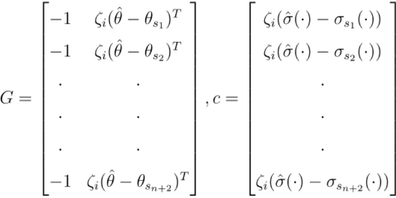
Lemma 3. Let 𝑠𝑔𝑛(𝑒𝑐)𝑠𝑔𝑛(𝜆𝑖) = 𝜁𝑖 𝑎𝑖 = ⎧ ⎪ ⎨ ⎪ ⎩ 𝜆𝑚𝑎𝑥𝐴1 if 𝜁𝑖𝜎(·) is convex on Θ𝑠 0 if 𝜁𝑖𝜎(·) is concave on Θ𝑠 𝜔_𝑖* = ⎧ ⎪ ⎨𝐴₂ if 𝜁_𝑖𝜎(·) is convex on Θ_𝑠

where 𝐴 = [𝐴1, 𝐴2]𝑇 = 𝐺−1𝑐, 𝐴1 is a scalar and 𝐴2 ∈ R𝑛+1, 𝐺 = ⎡ ⎢ ⎢ ⎢ ⎢ ⎢ ⎢ ⎢ ⎢ ⎢ ⎢ ⎢ ⎢ ⎣ −1 𝜁𝑖(ˆ𝜃 − 𝜃𝑠1) 𝑇 −1 𝜁𝑖(ˆ𝜃 − 𝜃𝑠2) 𝑇 · · · · · · −1 𝜁𝑖(ˆ𝜃 − 𝜃𝑠𝑛+2) 𝑇 ⎤ ⎥ ⎥ ⎥ ⎥ ⎥ ⎥ ⎥ ⎥ ⎥ ⎥ ⎥ ⎥ ⎦ , 𝑐 = ⎡ ⎢ ⎢ ⎢ ⎢ ⎢ ⎢ ⎢ ⎢ ⎢ ⎢ ⎢ ⎢ ⎣ 𝜁𝑖(ˆ𝜎(·) − 𝜎𝑠1(·)) 𝜁𝑖(ˆ𝜎(·) − 𝜎𝑠2(·)) · · · 𝜁𝑖(ˆ𝜎(·) − 𝜎𝑠𝑛+2(·)) ⎤ ⎥ ⎥ ⎥ ⎥ ⎥ ⎥ ⎥ ⎥ ⎥ ⎥ ⎥ ⎥ ⎦

The sliding mode component of (2.19) is defined as:

𝑢𝑠𝑙= −𝑀 (𝑋𝑝)𝑠𝑎𝑡

(︁𝑒_𝑐 𝜖

)︁

(2.30)

where 𝑀 (·) is defined as in (2.7). 𝑐(𝑡) in (2.19) is given by

𝑐(𝑡) = 𝑚𝑎𝑥 (︃ 0, 𝑠𝑎𝑡 (︃_||𝑋𝑝|| 𝑅 − 1 𝛿 )︃)︃ (2.31)

The reasoning behind the choice of the control input as in (2.19) is as follows. The first term corresponds to the baseline controller and leverages the prior information available about the linear plant dynamics in the form of 𝐴𝑝. The sliding mode control

input is necessary to ensure global boundedness even in the presence of the state dependent disturbance 𝜖0(𝑋𝑝) in (2.5). The second term is the main adaptive control

component where, in addition to the usual linear parameters ˆ𝜆𝑖 and ˆ𝑤𝑖 that are

normally included in adaptive controllers, we also propose to estimate the nonlinear parameters ˆ𝜃𝑖 using the approach suggested in [6]. We then proceed to show the

global boundedness of the parameter estimates while ensuring a small tracking error. Fig. 2-1 shows a block diagram to succinctly summarize the controller design.

Remark 1. The choice of 𝑐(𝑡) as in (2.31) ensures that the control input is continuous and enables a smooth transition between 𝑢𝑎𝑑 and 𝑢𝑠𝑙. Similarly, the choice of 𝑠(·) as

Figure 2-1: Block diagram of the proposed controller

2.5.1

Underlying Error Model

In order to show that the controller in (2.19) guarantees boundedness, we will adopt an error model approach. With the definitions of the underlying errors as in (2.9), it can be shown using (2.1), (2.2) and (2.19) that the error dynamics of 𝐸 is of the form

˙

𝐸 = 𝐴𝑚𝐸 + 𝑏 ((1 − 𝑐)𝑢𝑎𝑑+ 𝑐𝑢𝑠𝑙+ 𝑓 ) (2.32)

Using (2.10) and (2.32), the error dynamics for the composite error 𝑒𝑐can be written

as:

˙𝑒𝑐 = −𝑘𝑒𝑐+ (1 − 𝑐)𝑢𝑎𝑑+ 𝑚𝑢𝑠𝑙+ 𝑓 (2.33)

The following lemmas are useful in proving the main result.

Proof of Lemma 4. When 𝑋𝑝 ∈ 𝒟, then 𝑐 = 0. Thus we have:

𝑐(𝑢𝑠1+ 𝑓 )𝑒𝜖 = 0

When, 𝑋𝑝 ∈ 𝒟𝑐, then 0 < 𝑐 ≤ 1. Now we have,

(𝑢𝑠𝑙+ 𝑓 )𝑒𝜖 ≤ 𝑢𝑠𝑙𝑒𝜖+ |𝑓 ||𝑒𝜖|

≤ −𝑀 (𝑋𝑝)|𝑒𝜖| + |𝑓 ||𝑒𝜖|

The choice of 𝑀 (𝑋𝑝) as in (2.7) guarantees,

(𝑢𝑠𝑙+ 𝑓 )𝑒𝜖 ≤ 0 Thus we have, 𝑐(𝑢𝑠𝑙+ 𝑓 )𝑒𝜖 ≤ 0 Lemma 5. When |𝑒𝑐| > 𝑔𝜖, (︃ − 𝑛𝑓 ∑︁ 𝑖=1 (︁^_{𝜆𝑖𝜎(^𝜃}𝑇 𝑖 𝑋¯𝑝) )︁ + 𝑛𝑓 ∑︁ 𝑖=1 (︀𝜆𝑖𝜎(𝜃𝑖𝑇𝑋¯𝑝) )︀ )︃ 𝑒𝜖 − 𝑛𝑓 ∑︁ 𝑖=1 𝑎𝑖𝑠 (︂ 𝑒𝑐 𝑔𝜖 )︂ 𝑒𝜖+ 𝑛𝑓 ∑︁ 𝑖=1 (︁˜_{𝜆𝑖𝜎( ^𝜃𝑖}𝑇 _¯ 𝑋𝑝)𝑒𝜖+ 𝜆𝑖𝜃˜𝑖𝑇𝜔𝑖𝑒𝜖 )︁ ≤ 0

Proof of Lemma 5. For any 𝑖 let 𝐿𝑖 be given as:

𝐿𝑖 = (︂ −^𝜆𝑖𝜎(^𝜃𝑇𝑖 𝑋¯𝑝) + 𝜆𝑖𝜎(𝜃𝑇𝑖 𝑋¯𝑝) − 𝑎𝑖𝑠 (︂ 𝑒𝑐 𝑔𝜖 )︂)︂ 𝑒𝜖 +(︁˜𝜆𝑖𝜎( ^𝜃𝑖 𝑇 _¯ 𝑋𝑝)𝑒𝜖+ |𝜆𝑖|˜𝜃𝑇𝑖 𝑠𝑔𝑛(𝜆𝑖)𝜔𝑖𝑒𝜖 )︁ 𝐿𝑖 = (︂ −^𝜆𝑖𝜎(^𝜃𝑇𝑖 𝑋¯𝑝) + ˜𝜆𝑖𝜎( ^𝜃𝑖 𝑇 _¯ 𝑋𝑝) + 𝜆𝑖𝜎(𝜃𝑖𝑇𝑋¯𝑝) − 𝑎𝑖𝑠 (︂ 𝑒𝑐 𝑔𝜖 )︂ + 𝜆𝑖𝜃˜𝑇𝑖 𝜔𝑖 )︂ 𝑒𝜖

Using the definition of ˜𝜆𝑖 as in (2.9), for |𝑒𝑐| > 𝑔𝜖, we get 𝐿𝑖 = (︁ 𝜆𝑖 (︁ 𝜎(𝜃𝑇_𝑖 𝑋¯𝑝) − 𝜎(^𝜃𝑖𝑇𝑋¯𝑝) + ˜𝜃𝑖𝑇𝜔𝑖 )︁ − 𝑎𝑖𝑠𝑔𝑛(𝑒𝜖) )︁ 𝑒𝜖

Using the definition of 𝐽𝑖 as in (2.25), we get

= (|𝜆𝑖|𝐽𝑖− 𝑎𝑖𝑠𝑔𝑛(𝑒𝜖)) 𝑒𝜖

By the choice of 𝑎𝑖 as in (2.23), we have 𝐿𝑖 ≤ 0 when

|𝑒𝑐| > 𝑔𝜖

2.6

Stability and Tracking

Theorem 1. Let assumptions 1-5 hold. Then for the plant in (2.1), the reference model in (2.2), using the controller specified in (2.19)-(2.31), the closed loop system has globally bounded solutions and the tracking error 𝐸(𝑡) satisfies the bound

||𝐸(𝑡)|| ≤ 𝑘0max

(︁𝜖_𝑓

𝑘 + 𝜖, 𝑔𝜖 )︁

∀𝑡 > 𝑡0+ 𝑇 (2.34)

where 𝑇 is a finite positive constant.

Remark 2. The main difference between the adaptive controller in [13] and the one in (2.19)-(2.31) is the algorithm used for adjusting the nonlinear weights ˆ𝜃𝑖. In [13],

a linearization of the nonlinear weights is utilized and only the linear components are adjusted, which leads to additional nonlinear approximation errors. A stabilizing sliding-mode component is used to upper-bound these errors, which can hinder adap-tation of parameters. Instead, here we utilize a min-max algorithm that is based on convex/concave parameterization. The second difference is in the activation function. A ReLU activation function is proposed here to meet the convexity requirement, while a sigmoidal function is proposed in [13].

ReLU, but the more important distinction is that the centers, which occur nonlinearly, are fixed. Instead, in our controller, we adjust the nonlinear parameters as well. As will be shown in the simulation section, this leads to better learning of the parameters and therefore the underlying nonlinearity.

Remark 4. Perhaps the most restrictive assumption made for the proof of Theorem 1 is in Assumption (3), where we require the signs of the linear weights to be known. In some cases, there may be sufficient information available about the underlying nonlinearity that may permit these signs to be known. The simulation example included in Section V corresponds to such a nonlinearity.

Proof of Theorem 1. Consider the candidate Lyapunov function

𝑉 = 1 2 (︃ 𝑒2_𝜖 + 𝑛𝑓 ∑︁ 𝑖=1 (︁ Γ−1_^ 𝜆𝑖 ˜ 𝜆2_𝑖 + |𝜆𝑖|˜𝜃𝑇𝑖 Γ −1 ^ 𝜃𝑖 ˜ 𝜃𝑖+ Γ−1𝑤^𝑖𝑤˜ 2 𝑖 )︁ )︃ when |𝑒𝑐| > 𝜖 ˙ 𝑉 = ˙𝑒𝑐𝑒𝜖+ 𝑛𝑓 ∑︁ 𝑖=1 (︁ Γ−1_^ 𝜆𝑖 ˜ 𝜆𝑖˙˜𝜆𝑖+ |𝜆𝑖|˜𝜃𝑖𝑇Γ −1 ^ 𝜃𝑖 ˙˜ 𝜃𝑖+ Γ−1𝑤^𝑖𝑤˜𝑖𝑤˙˜𝑖 )︁ ˙ 𝑉 ≤ −𝑘𝑒2 𝜖 + 𝑒𝜖((1 − 𝑐)𝑢𝑎𝑑+ 𝑚𝑢𝑠𝑙+ 𝑓 ) + 𝑛𝑓 ∑︁ 𝑖=1 (︁ Γ−1_^ 𝜆𝑖 ˜ 𝜆𝑖˙˜𝜆𝑖+ |𝜆𝑖|˜𝜃𝑖𝑇Γ −1 ^ 𝜃𝑖 ˙˜ 𝜃𝑖+ Γ−1𝑤^𝑖𝑤˜𝑖𝑤˙˜𝑖 )︁

Substituting the control input from (2.21), (2.30)

˙ 𝑉 ≤ −𝑘𝑒2_𝜖 + 𝑒𝜖(1 − 𝑐) (︃ − 𝑛𝑓 ∑︁ 𝑖=1 𝑎𝑖𝑠 (︂ 𝑒𝑐 𝑔𝜖 )︂ + 𝜖(𝑋𝑝) )︃ +𝑒𝜖(1 − 𝑐) (︃ − 𝑛𝑓 ∑︁ 𝑖=1 (︁^_{𝜆𝑖𝜎𝑖(^𝜃}𝑇 𝑖 𝑋¯𝑝) + ^𝑤𝑖 )︁ )︃ +𝑒𝜖(1 − 𝑐) (︃𝑛𝑓 ∑︁ 𝑖=1 (︀𝜆𝑖𝜎(𝜃𝑖𝑇𝑋¯𝑝) + 𝑤𝑖 )︀ )︃ + 𝑛𝑓 ∑︁ 𝑖=1 (︁ Γ−1_^ 𝜆𝑖 ˜ 𝜆𝑖˙˜𝜆𝑖+ |𝜆𝑖|˜𝜃𝑖𝑇Γ−1_𝜃^_𝑖 𝜃˙˜𝑖+ Γ −1 ^ 𝑤𝑖𝑤˜𝑖𝑤˙˜𝑖 )︁ +𝑐(︁−𝑀 (𝑋_𝑝)𝑠𝑎𝑡(︁𝑒𝑐 𝜖 )︁ + 𝑓1 )︁ 𝑒𝜖

Substituting the update laws from (2.26)-(2.28) ˙ 𝑉 ≤ −𝑘𝑒2_𝜖− 𝑒𝜖(1 − 𝑐) (︃𝑛𝑓 ∑︁ 𝑖=1 𝑎𝑖𝑠 (︂ 𝑒𝑐 𝑔𝜖 )︂)︃ +𝑒𝜖(1 − 𝑐) (︃ − 𝑛𝑓 ∑︁ 𝑖=1 (︁^_{𝜆𝑖𝜎𝑖(^𝜃}𝑇 𝑖 𝑋¯𝑝) + ^𝑤𝑖 )︁ )︃ +𝑒𝜖(1 − 𝑐) (︃𝑛𝑓 ∑︁ 𝑖=1 (︀𝜆𝑖𝜎(𝜃𝑇𝑖 𝑋¯𝑝) + 𝑤𝑖 )︀ )︃ + 𝑛𝑓 ∑︁ 𝑖=1 (1 − 𝑐)˜𝜆𝑖Γ−1_𝜆^ 𝑖 𝑃 𝑟𝑜𝑗Γ_𝜆𝑖^ (︁^𝜆𝑖, 𝜎(^𝜃 𝑇 𝑖 𝑋¯𝑝)𝑒𝜖 )︁ + 𝑛𝑓 ∑︁ 𝑖=1 (1 − 𝑐)|𝜆𝑖|˜𝜃𝑇𝑖 Γ−1_𝜃^_𝑖 𝑃 𝑟𝑜𝑗Γ_𝜃𝑖^ (︁ ^𝜃𝑖, 𝑠𝑔𝑛(𝜆𝑖)𝜔 * 𝑖𝑒𝜖 )︁ + 𝑛𝑓 ∑︁ 𝑖=1 (1 − 𝑐) ˜𝑤𝑖Γ−1_𝑤^𝑖𝑃 𝑟𝑜𝑗Γ_𝑤𝑖^ ( ^𝑤𝑖, 𝑒𝜖) +𝑐(︁−𝑀 (𝑋_𝑝)𝑠𝑎𝑡(︁𝑒𝑐 𝜖 )︁ + 𝑓1 )︁ 𝑒𝜖+ (1 − 𝑐)(𝜖(𝑋𝑝))𝑒𝜖

When 𝑋𝑝 ∈ 𝒟𝑐𝛿, we have 𝑐 = 1. The choice of 𝑀 (𝑋𝑝) as in (2.7), guarantees that

˙

𝑉 < −𝑘𝑒2_𝜖 (2.35) As 𝑋𝑝= 𝐸 + 𝑋𝑚, (2.35) implies that 𝑋𝑝 ∈ 𝒟𝛿 ∀𝑡 > 𝑡0+ 𝑇1 for some finite 𝑇1.

When 𝑋𝑝 ∈ 𝒟𝛿, using Lemma 2, we have, ˙ 𝑉 ≤ −𝑘𝑒2_𝜖− 𝑒_𝜖(1 − 𝑐) (︃𝑛_𝑓 ∑︁ 𝑖=1 𝑎𝑖𝑠 (︂ 𝑒𝑐 𝑔𝜖 )︂)︃ +𝑒𝜖(1 − 𝑐) (︃ − 𝑛𝑓 ∑︁ 𝑖=1 (︁^_{𝜆𝑖𝜎𝑖(^𝜃}𝑇 𝑖 𝑋¯𝑝) + ^𝑤𝑖 )︁ )︃ +𝑒𝜖(1 − 𝑐) (︃𝑛𝑓 ∑︁ 𝑖=1 (︀𝜆𝑖𝜎(𝜃𝑇𝑖 𝑋¯𝑝) + 𝑤𝑖 )︀ )︃ + 𝑛𝑓 ∑︁ 𝑖=1 (1 − 𝑐)˜𝜆𝑖𝜎(^𝜃𝑇𝑖 𝑋¯𝑝)𝑒𝜖 + 𝑛𝑓 ∑︁ 𝑖=1 (1 − 𝑐)𝜆𝑖𝜃˜𝑇𝑖 𝜔 * 𝑖𝑒𝜖 + 𝑛𝑓 ∑︁ 𝑖=1 (1 − 𝑐) ˜𝑤𝑖𝑒𝜖 +𝑐 (︁ −𝑀 (𝑋𝑝)𝑠𝑎𝑡 (︁𝑒_𝑐 𝜖 )︁ + 𝑓1 )︁ 𝑒𝜖+ (1 − 𝑐)(𝜖(𝑋𝑝))𝑒𝜖

Now using lemmas 4 and 5 ˙ 𝑉 ≤ −𝑘𝑒2_𝜖 + (1 − 𝑐)𝜖(𝑋𝑝)𝑒𝜖 ≤ −𝑘𝑒2_𝜖 + 𝜖𝑓|𝑒𝜖| when |𝑒_𝜖| > 𝜖𝑓 𝑘, ˙ 𝑉 < 0

Thus ˙𝑉 < 0 outside a compact set 𝒞. The compact set may be defined as: 𝒞 = (|𝑒𝜖| ≤ 𝑚𝑎𝑥 (︁𝜖_𝑓 𝑘, (𝑔 − 1)𝜖 )︁ , |˜𝜆𝑖| ≤ 2|𝜆|𝑚𝑎𝑥+ 𝜂𝜆, ||˜𝜃𝑖|| ≤ 2 √ 𝑛 + 1𝜃𝑚𝑎𝑥+ 𝜂𝜃, | ˜𝑤𝑖| ≤ 2|𝑤|𝑚𝑎𝑥+ 𝜂𝑤)

This implies that ∀𝑡 > 𝑡0+ 𝑇2 for some finite 𝑇2 > 𝑇1,

|𝑒𝜖(𝑡)| ≤ 𝑚𝑎𝑥

(︁𝜖_𝑓

𝑘, (𝑔 − 1)𝜖 )︁

From (2.11) and (2.36), we have a bound on the composite error: |𝑒𝑐(𝑡)| ≤ 𝑚𝑎𝑥 (︁𝜖_𝑓 𝑘 + 𝜖, 𝑔𝜖 )︁ ∀𝑡 > 𝑡0+ 𝑇2 Using lemma 1, ||𝐸(𝑡)|| ≤ 𝑘₀𝑚𝑎𝑥(︁𝜖𝑓 𝑘 + 𝜖, 𝑔𝜖 )︁ ∀𝑡 > 𝑡₀+ 𝑇2 𝑅 in (2.17) guarantees 𝑋𝑝∈ 𝒟 ∀𝑡 > 𝑡0+ 𝑇2

2.6.1

An Alternate Non-adaptive Controller

In order to illustrate that the bound derived in (3.19) is small, we describe an alternate non-adaptive controller in this section. The alternate controller is chosen of the form

𝑢 = 𝑢𝑏𝑙+ 𝜃𝑔𝑢𝑠𝑙 (2.37)

where 𝑢𝑏𝑙 is chosen as in (2.20) and 𝑢𝑠𝑙 is given by

𝑢𝑠𝑙 = ⎧ ⎪ ⎨ ⎪ ⎩ −𝑀 (𝑋𝑝)𝑠𝑎𝑡(𝑒_𝜖𝑐) when 𝑋𝑝 ∈ 𝒟𝑐 −𝑚0𝑠𝑎𝑡(𝑒_𝜖𝑐) when 𝑋𝑝 ∈ 𝒟 (2.38)

We will derive a corresponding bound to (3.19) that can be achieved with this non-adaptive controller in Proposition 1. The following definitions are useful:

𝐸𝑎𝑑 = 𝑘0max (︁𝜖_𝑓 𝑘 + 𝜖, 𝑔𝜖 )︁ (2.39) 𝐸𝑠𝑙= 𝑚𝑖𝑛 (︂ 𝑅 + 𝑋𝑚0, 𝑘0 (︂ 𝑀1− 𝑚0 𝑘 + 𝜖 )︂)︂ (2.40)

Proposition 1. Let the nonlinearity in (2.1) satisfy Assumption 4 with 𝑅 satisfying inequality (2.17) and 𝑀1 satisfying inequality (2.18) Then,

(2.38) leads to a closed loop system that has globally bounded solutions and leads to a tracking error 𝐸(𝑡) that satisfies the bound

||𝐸(𝑡)|| ≤ 𝐸𝑠𝑙 ∀𝑡 > 𝑡0+ 𝑇𝑠 (2.41)

for a finite 𝑇𝑠.

b) 𝐸𝑠𝑙> 𝐸𝑎𝑑.

Proposition 1b) is an important contribution of this thesis, as it proves that the proposed adaptive controller achieves better error tracking compared to the alternate non-adaptive controller.

Proof of Proposition 1. Consider the candidate Lyapunov function

𝑉 = 1 2𝑒 2 𝜖 ˙ 𝑉 ≤ −𝑘𝑒2 𝜖 + 𝑒𝜖(𝑢𝑠𝑙+ 𝑓 ) When 𝑋𝑝 ∈ 𝒟𝑐, we have ˙ 𝑉 ≤ −𝑘𝑒2 𝜖 − |𝑒𝜖|𝑀 (𝑋𝑝) + |𝑓 ||𝑒𝜖| ˙ 𝑉 ≤ −2𝑘𝑉 − ∆

from assumption 4. This implies that

𝑉 (𝑡) ≤ 𝑉 (𝑡0)𝑒𝑥𝑝 (−2𝑘(𝑡 − 𝑡0)) (2.42)

As 𝑋𝑝 = 𝐸 + 𝑋𝑚, (2.42) implies that 𝑋𝑝(𝑡) ∈ 𝒟 ∀𝑡 ≥ 𝑡0+ 𝑇3 for some finite 𝑇3. This

guarantees global boundedness and we have,

||𝐸|| ≤ 𝑅 + 𝑋𝑚0 (2.43)

When 𝑋𝑝 ∈ 𝒟, we have

˙

𝑉 ≤ −𝑘𝑒2_𝜖 − |𝑒𝜖|𝑚0+ |𝑓 ||𝑒𝜖|

Thus ˙𝑉 < 0 outside a compact set 𝒮,

𝒮 = (︂ |𝑒𝜖| ≤ 𝑀1− 𝑚0 𝑘 )︂

This implies that,

|𝑒𝜖(𝑡)| ≤

𝑀1− 𝑚0

𝑘 ∀𝑡 ≥ 𝑡0+ 𝑇4 (2.44)

for some finite time 𝑇4 > 𝑇3 and therefore that,

||𝐸(𝑡)|| ≤ 𝑘0 (︂ 𝑀1− 𝑚0 𝑘 + 𝜖 )︂ ∀𝑡 ≥ 𝑡0+ 𝑇4 (2.45) Using (2.45), ||𝑋𝑝|| ≤ 𝑘0 (︂ 𝑀₁ − 𝑚0 𝑘 + 𝜖 )︂ + 𝑋𝑚0 if 𝑅 < 𝑘0 (︀_{𝑀1−𝑚0}

𝑘 + 𝜖)︀ + 𝑋𝑚0, 𝑋𝑝 cannot be guaranteed to remain in the interior of

𝒟. Using (2.43), (2.45), we get ∀𝑡 ≥ 𝑡0 + 𝑇4 ||𝐸(𝑡)|| ≤ 𝑚𝑖𝑛 (︂ 𝑅 + 𝑋𝑚0, 𝑘0 (︂ 𝑀1− 𝑚0 𝑘 + 𝜖 )︂)︂ (2.46)

2.7

Simulation Results

We implement the adaptive controller proposed in this chapter on the automatic landing system for a medium-size transport aircraft academic example presented in

ground-effect phenomenon. The plant model for the aircraft is obtained using linear dynamics at 300 ft. and a true airspeed of 250 ft/s. The ground effect phenomenon is embedded into the linear model and we obtain the following plant dynamics:

⎡ ⎢ ⎢ ⎢ ⎢ ⎢ ⎢ ⎢ ⎢ ⎢ ⎣ ˙ 𝑉 ˙ 𝛼 ˙ 𝑞 ˙ 𝜃 ˙ℎ ⎤ ⎥ ⎥ ⎥ ⎥ ⎥ ⎥ ⎥ ⎥ ⎥ ⎦ ⏟ ⏞ ˙ 𝑋𝑝 = ⎡ ⎢ ⎢ ⎢ ⎢ ⎢ ⎢ ⎢ ⎢ ⎢ ⎣ −0.038 18.984 0 −32.174 0 −0.001 −0.632 1 0 0 0 −0.759 −0.518 0 0 0 0 1 0 0 0 −250 0 250 0 ⎤ ⎥ ⎥ ⎥ ⎥ ⎥ ⎥ ⎥ ⎥ ⎥ ⎦ ⏟ ⏞ 𝐴𝑝 ⎡ ⎢ ⎢ ⎢ ⎢ ⎢ ⎢ ⎢ ⎢ ⎢ ⎣ 𝑉 𝛼 𝑞 𝜃 ℎ ⎤ ⎥ ⎥ ⎥ ⎥ ⎥ ⎥ ⎥ ⎥ ⎥ ⎦ ⏟ ⏞ 𝑋𝑝 + ⎡ ⎢ ⎢ ⎢ ⎢ ⎢ ⎢ ⎢ ⎢ ⎢ ⎣ 10.1 0 0 −0.0086 0.025 −0.011 0 0 0 0 ⎤ ⎥ ⎥ ⎥ ⎥ ⎥ ⎥ ⎥ ⎥ ⎥ ⎦ ⏟ ⏞ 𝐵𝑝 ⎡ ⎣ 𝛿𝑡ℎ 𝛿𝑒 ⎤ ⎦ ⏟ ⏞ 𝑢 + ⎡ ⎢ ⎢ ⎢ ⎢ ⎢ ⎢ ⎢ ⎢ ⎢ ⎣ −18.984 0.632 0.759 0 0 ⎤ ⎥ ⎥ ⎥ ⎥ ⎥ ⎥ ⎥ ⎥ ⎥ ⎦ ⏟ ⏞ 𝐵𝑔 𝛼𝑔(ℎ) Further, we re-write 𝐵𝑔 as 𝐵𝑔 = 𝐵𝑝 ⎡ ⎣ −1.8796 −73.2718 ⎤ ⎦ ⏟ ⏞ 𝜃𝑔

and restate the plant dynamics in the form of (2.1). The regulated output is related to the plant dynamics as:

𝑌 = ⎡ ⎣ 𝑉 ℎ ⎤ ⎦= 𝐶𝑋𝑝 𝐶 = ⎡ ⎣ 1 0 0 0 0 0 0 0 0 1 ⎤ ⎦

The commands for this auto-landing problem consists of a true airspeed command and an altitude command as:

𝑟 = ⎡ ⎣ 𝑉𝑐𝑚𝑑 ℎ𝑐𝑚𝑑 ⎤ ⎦

Consistent with the assumption made in Section II, we assume that 𝐴𝑝, 𝐵𝑝 and 𝜃𝑔 are

known, but the ground effect is unknown. For the simulation studies reported below, we assume that the ground effect is of the form

𝛼𝑔(ℎ) = −

4𝜋

180(1 − tanh (0.1(ℎ − 60))) (2.47)

2.7.1

Baseline Controller (BC)

A baseline control input is defined as

𝑢𝑏𝑙 = −𝐾𝑥𝑇𝑋𝑝+ 𝐾𝑟𝑇𝑟 (2.48)

where 𝐾𝑥 and 𝐾𝑟 are baseline feedback and feedforward gains determined using the

LQR method, respectively. The feedforward gain 𝐾𝑟 ensures an identity DC gain for

the baseline closed loop system from 𝑟 to 𝑌 . For the numerical values mentioned earlier, these were computed as

𝐾_𝑥𝑇 = ⎡ ⎣ 0.1173 −89.1740 42.8761 140.0007 0.2340 0.0186 −40.6065 4.3798 58.6016 0.2127 ⎤ ⎦ 𝐾_𝑟𝑇 = ⎡ ⎣ −0.7753 0.2340 ⎤ ⎦

Thus the closed loop reference model is given as ˙ 𝑋𝑚 = (𝐴𝑝− 𝐵𝑝𝐾𝑥𝑇) ⏟ ⏞ 𝐴𝑚 𝑋𝑚+ 𝐵𝑝𝐾𝑟𝑇𝑟 (2.49)

2.7.2

A comparable fixed adaptive controller (FAC)

In order to evaluate the performance of the proposed adaptive controller based on nonlinear parameterization, we choose a different adaptive controller modified from that in Chapter 12, page 382 in [20], which considered a neural network approxima-tion where the activaapproxima-tion funcapproxima-tions were chosen to be radial basis funcapproxima-tions whose nonlinear weights were fixed and only linear weights were adjusted. The modified version of this controller is described below:

𝑢 = 𝑢𝑏𝑙+ 𝜃𝑔𝑢𝑎𝑑 (2.50) where, 𝑢𝑎𝑑 = −ˆ𝜃𝑇𝜑(ℎ) 𝜑(ℎ) = [︁ 𝜑1(ℎ) 𝜑2(ℎ) 𝜑3(ℎ) 𝜑4(ℎ) 𝜑5(ℎ) 1 ]︁𝑇 𝜑𝑖 = 𝑒𝑥𝑝(−0.0056(ℎ − ℎ𝑖)2), 𝑖 = 1, ..., 5 ˙ˆ𝜃 = 𝑃𝑟𝑜𝑗Γ𝜃(ˆ𝜃, 𝜑(ℎ)𝐸 𝑇 𝑃 𝑏)

𝑃 is obtained by solving the Lyapunov equation and 𝑢𝑏𝑙 is as described in (2.48). The

nonlinear parameters which correspond to the centers ℎ𝑖 for the radial basis functions

𝜑𝑖 are (−20, 0, 20, 40, 60) for 𝑖 = 1, ..., 5 respectively. Main difference between the

adaptive controller in [20] and (2.50) is that 𝜃𝑔 is assumed to be known in the above

formulation. Since the nonlinear parameters are fixed in this controller, we denote it as a fixed-adaptive controller.

2.7.3

Proposed nonlinear adaptive controller (NLAC)

The nonlinear-adaptive controller proposed in this thesis specified in (2.19)-(2.31) was simulated together with the plant and reference model described above. A ReLU activation function [17] was chosen, with 𝑛𝑓 in (2.21) set to 5, similar to the number

of basis functions in the fixed-adaptive controller. We assumed that 𝑠𝑔𝑛(𝜆𝑖) = −1

for 𝑖 = 1, . . . , 3 and that 𝑠𝑔𝑛(𝜆4), 𝑠𝑔𝑛(𝜆5) = 1. This assumption is reasonable and

was made based on the shape of the ground-effect. Also, we chose the bounds on the parameters to be 𝜃𝑚𝑎𝑥 = 5, 𝜆𝑚𝑎𝑥 = 10 and 𝑤𝑚𝑎𝑥 = 1. We chose 𝑔 and 𝜖 in (2.21)

to be 5 and 10−3 respectively. 𝛽 in (2.22) was chosen to be 4. Note that the ground effect is absent at high altitudes and thus we do not require 𝑢𝑠𝑙.

2.7.4

A linearized adaptive controller (LAC)

In literature, an adaptive neural controller where the non-linear parameters are tuned has been proposed [13]. As stated in remark 2, a linearization of the nonlinear param-eters combined with a robustifying term is used to develop such an adaptive neural controller. In this subsection, we briefly propose such a linearized controller. The controller performance in approximating the nonlinearity will be compared to the proposed nonlinear adaptive controller proposed in this thesis.

The control input is a combination of a baseline controller, an adaptive controller and a sliding mode controller.

𝑢 = 𝑢𝑏𝑙 + 𝜃𝑔((1 − 𝑐)𝑢𝑎𝑑+ 𝑚𝑢𝑠𝑙) 𝑢𝑏𝑙 = 𝐾𝑋𝑝+ 𝑟 𝑢𝑎𝑑 = − 𝑛𝑓 ∑︁ 𝑖=1 (︁ˆ𝜆𝑖𝜎(ˆ𝜃𝑇𝑖 𝑋¯𝑝) + ˆ𝑤𝑖 )︁ − 𝑢𝑟 𝑢𝑟 = 𝐾𝑟𝑜𝑏 ⎛ ⎝ ⎯ ⎸ ⎸ ⎷ 𝑛𝑓 ∑︁ 𝑖=1 (︁ˆ𝜆2 𝑖 + ˆ𝜃𝑖2 )︁ + 𝑛𝑓 √︀ 𝜆2 𝑚𝑎𝑥+ 𝜃2𝑚𝑎𝑥 ⎞ ⎠ (︁𝑒_𝑐)︁

The parameter update laws are: ˙ˆ𝜆_𝑖 = 𝜎(ˆ𝜃𝑇_𝑖 𝑋¯𝑝)𝑒𝑐− 𝜎 ′ (ˆ𝜃𝑇_𝑖 𝑋¯𝑝)ˆ𝜃𝑖𝑇𝑋¯𝑝𝑒𝑐− 𝜅𝑒𝑐ˆ𝜆𝑖 ˙ˆ𝜃_𝑖 = ˆ𝜆𝑖𝜎 ′ (ˆ𝜃𝑇𝑋¯𝑝)𝑒𝑐𝑋¯𝑝− 𝜅𝑒𝑐𝜃ˆ𝑖 ˙ˆ 𝑤𝑖 = 𝑒𝑐

It can be shown that the controller design along-with the update laws is stable and can track the reference signal with a small tracking error. The update laws and main idea of linearizing the nonlinear weight updates is similar to the one in [13]. For more details, the reader is referred to the same.

One key aspect to consider while evaluating the function approximation perfor-mance of the controllers is the initialization of nonlinear parameters. The proposed nonlinear adaptive controller and the linearized adaptive controller use different acti-vation functions and thus an exact equivalent initialization of the nonlinear parame-ters is impossible. In-order to draw a comparison between the effectiveness of the two controllers in tuning the nonlinear parameters, we compare the performance of the two controllers to their analogs wherein the nonlinear parameters were fixed to their initialized values. More precisely, we simulate two additional controllers NLAC-fw and LAC-fw, wherein the nonlinear parameters are fixed to their initial values and only the linear parameters are tuned.

The results of the closed-loop responses using the proposed nonlinear-adaptive controller, the fixed-adaptive controller and the linearized adaptive controller are shown in Fig. 2-2 through fig. 2-13. For comparison, we also show the reference signals and the responses from the non-adaptive baseline controller 𝑢𝑏𝑙 described in

(2.48). To illustrate the effectiveness of tuning the nonlinear parameters, we also show the response of the nonlinear adaptive controller and the linearized adaptive controller when the nonlinear parameters are fixed to their initial values.

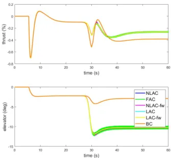
Figs. 2-2 through 2-4 illustrate the outputs of interest, speed and altitude, the control inputs, thrust and elevator, and the estimated nonlinear component respec-tively. It is evident from fig. 2-2 that the aircraft is unable to land with only the

baseline controller. All other adaptive controllers are able to successfully land the aircraft.

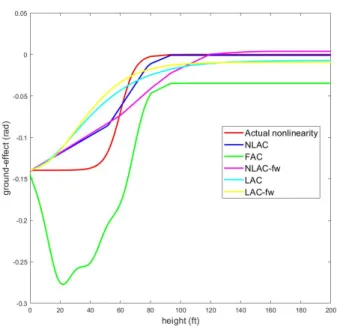
Inorder to evaluate the function approximation capacities of each controller, we simulate the controllers over multiple landings. The parameters learnt at the end of each landing are used as initial parameters for the next landing. From fig. 2-4, 2-7, 2-10 and 2-13, it is clear that the nonlinear adaptive controller is able to approxi-mate the unknown ground-effect better than the other adaptive controllers and its approximation performance improves with each successive landing. By comparing the performance of the NLAC to NLAC-fw , we can conclude that tuning the nonlin-ear parameters results in better approximation of the nonlinnonlin-earity. Finally, we also conclude that the proposed nonlinear adaptive controller has better approximation capabilities as compared to that of a linearized adaptive controller.

Figure 2-3: One Landing: Control Inputs of different controllers

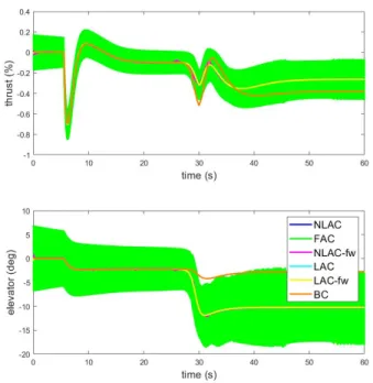
Figure 2-5: Five Landings: Tracking performance of controllers

Figure 2-7: Five Landings: Learning performance of different controllers

Figure 2-9: Fifteen Landings: Control Inputs of different controllers

Figure 2-11: Thirty Landings: Tracking performance of controllers

Chapter 3

Nonlinear Adaptive

Controller-Extension

3.1

Introduction

In the previous chapter, we proposed a neural network based nonlinear adaptive controller for approximating a scalar non-linearity. In this chapter, we consider the extension to the problem where-in the unknown non-linearity is a vector. The chapter is organized as follows. In section 3.2, we restate the problem statement. Section 3.3 restates the error definitions. In section 3.4, we propose the controller design and establishes the error model used for analyzing the proposed controller. The development of the control input and update laws closely follows the approach stated in chapter 2 with a slightly different error model. Section 3.5 states the main theorem establishing the stability and tracking properties of the closed loop system with the proposed adaptive controller. In section 3.6, we implement the controller on the same auto-lander problem and document the performance of the proposed controller.

3.2

Problem Statement

We limit our consideration to plants with a matched nonlinearity as in (2.1). All parameters in (2.1) are assumed to be known except for 𝜃𝑔 and 𝑓 (𝑋𝑝). The objective

remains the same, namely designing a control input 𝑢 to have globally bounded solutions and the plant state 𝑋𝑝 tracking the state 𝑋𝑚 of the reference model in (2.2)

with a small tracking error. In addition to assumptions (1) to (5) listed in chapter 2, we assume that the signs of the individual elements of 𝜃𝑔 are known. More precisely

Assumption 6. let 𝜃𝑔 = [𝜃𝑔1, 𝜃𝑔2, ..., 𝜃𝑔𝑚]

𝑇_{. then the sign of 𝜃}

𝑔𝑗 for 𝑗 = 1, ..., 𝑚 is

known.

In-order to proceed with the controller design, we modify the neural network approximation in assumption (1) as follows.

𝜃𝑔𝑗𝑓 = 𝑛𝑓 ∑︁ 𝑖=1 (︀𝜆𝑖𝑗𝜎(𝜃𝑖𝑗𝑇𝑋) + 𝑤¯ 𝑖𝑗)︀ + 𝜖𝑗(𝑋) (3.1) |𝜖𝑗(𝑋)| ≤ ||𝜃𝑔||∞𝜖𝑓 (3.2)

We express the control input matrix 𝐵𝑝 in terms of its columns as:

𝐵𝑝 = [𝑏1, 𝑏2, ..., 𝑏𝑚] (3.3)

where 𝑏𝑗 ∈ R𝑛.

3.3

Error Definitions

The following error definitions would be useful in establishing the stability and track-ing performance of the controller.

𝐸 = 𝑋𝑝− 𝑋𝑚, ˜𝜆𝑖𝑗 = ˆ𝜆𝑖𝑗 − 𝜆𝑖𝑗, ˜𝜃𝑖𝑗 = ˆ𝜃𝑖𝑗 − 𝜃𝑖𝑗, ˜𝑤𝑖𝑗 = ˆ𝑤𝑖𝑗 − 𝑤𝑖𝑗 (3.4)

3.4

Controller design

Following a reasoning similar to the one outlined in chapter 2, we propose using the following control input

𝑢𝑏𝑙 = 𝐾𝑋𝑝+ 𝑟 (3.6) 𝑢𝑛𝑏𝑙 = [𝑢𝑛𝑏𝑙1, ..., 𝑢𝑛𝑏𝑙𝑚] 𝑇 _(3.7) 𝑢𝑛𝑏𝑙𝑗 = (1 − 𝑐(𝑡))𝑢𝑎𝑑𝑗+ 𝑐(𝑡)𝑢𝑠𝑙𝑗 (3.8) 𝑢𝑎𝑑𝑗 = − 𝑛𝑓 ∑︁ 𝑖=1 (︁ˆ𝜆𝑖𝑗𝜎(ˆ𝜃𝑇𝑖𝑗𝑋¯𝑝) + ˆ𝑤𝑖𝑗 )︁ − 𝑛𝑓 ∑︁ 𝑖=1 𝑎𝑖𝑗𝑠 (︂ 𝐸𝑇_{𝑃 𝑏} 𝑗 𝑔𝜖 )︂ (3.9) 𝑎𝑖𝑗 = 𝜆𝑚𝑎𝑥 min 𝜔𝑖∈R𝑛 max 𝜃𝑖∈Θ𝑠 𝑠𝑔𝑛(𝐸𝑇𝑃 𝑏𝑗)𝐽𝑖𝑗 (3.10) 𝜔*_𝑖𝑗 = arg. min 𝜔𝑖∈R𝑛 max 𝜃𝑖∈Θ𝑠 𝑠𝑔𝑛(𝐸𝑇𝑃 𝑏𝑗)𝐽𝑖𝑗 (3.11) 𝐽𝑖𝑗 = 𝑠𝑔𝑛(𝜆𝑖𝑗) (︁ 𝜎(𝜃_𝑖𝑗𝑇𝑋¯𝑝) − 𝜎(ˆ𝜃𝑖𝑗𝑇𝑋¯𝑝) + ˜𝜃𝑇𝑖𝑗𝜔𝑖𝑗 )︁ (3.12) 𝑢𝑠𝑙𝑗 = −||𝜃𝑔||∞𝑀 (𝑋𝑝)𝑠𝑎𝑡 (︂ 𝐸𝑇_{𝑃 𝑏} 𝑗 𝜖 )︂ (3.13) 𝑐(𝑡) = 𝑚𝑎𝑥 (︃ 0, 𝑠𝑎𝑡 (︃_||𝑋 𝑝|| 𝑅 − 1 𝛿 )︃)︃ (3.14)

where 𝑃 ∈ R𝑛×𝑛, a symmetric positive definite matrix is the solution to the Lyapunov equation:

𝐴𝑇_𝑚𝑃 + 𝑃 𝐴 = −𝑄, 𝑄 = 𝑄𝑇 > 0

The update laws are chosen as follows:

˙ˆ𝜆𝑖𝑗 = (1 − 𝑐)𝑃 𝑟𝑜𝑗Γ_𝜆𝑖𝑗^ (︁ˆ𝜆𝑖𝑗, 𝜎(ˆ𝜃 𝑇 𝑖 𝑋𝑝)𝐸𝑇𝑃 𝑏𝑗 )︁ (3.15) ˙ˆ𝜃_𝑖𝑗 = (1 − 𝑐)𝑃 𝑟𝑜𝑗Γ_𝜃𝑖𝑗^ (︁ ˆ𝜃𝑖𝑗, 𝑠𝑔𝑛(𝜆𝑖𝑗)𝜔 * 𝑖𝑗𝐸 𝑇 𝑃 𝑏𝑗 )︁ (3.16) ˙ˆ 𝑤𝑖𝑗 = (1 − 𝑐)𝑃 𝑟𝑜𝑗Γ_𝑤𝑖𝑗^ (︀ ˆ𝑤𝑖𝑗, 𝐸 𝑇_{𝑃 𝑏} 𝑗 )︀ (3.17)

We once again note that the update laws in (3.16) and (3.17), are the similar to update laws for linearly occurring parameters found in adaptive control literature whereas 𝜔_𝑖𝑗* is obtained by solving a min-max optimization problem.

3.4.1

Error Model

Inorder to study the stability and tracking properties of the proposed adaptive con-troller, we once again adopt an error model approach. Using the error definitions as stated in (3.4), along-with the plant and reference model dynamics as in (2.1),(2.2) and the control input as defined in (3.5), it can be shown that the error model is:

˙

𝐸 = 𝐴𝑚𝐸 + 𝐵𝑝(𝜃𝑔𝑓 + 𝑢𝑛𝑏𝑙) (3.18)

3.5

Stability and Tracking performance

Theorem 2. Let assumptions 1-6 hold. Then for the plant in (2.1), the reference model in (2.2), using the controller specified in (3.5)-(3.14), the closed loop system has globally bounded solutions and the tracking error 𝐸(𝑡) satisfies the bound

||𝐸(𝑡)|| ≤ 𝑚𝑎𝑥(︂ 2𝑚||𝑃 ||||𝑏𝑗||∞||𝜃𝑔||∞ 𝑄𝑚𝑖𝑛 , 𝑔𝜖 ||𝑃 ||||𝑏𝑗||𝑚𝑖𝑛 )︂ ∀𝑡 > 𝑡0+ 𝑇 (3.19)

where 𝑇 is a finite positive constant.

Proof of Theorem 2. Consider the candidate Lyapunov function

𝑉 = 1 (︃ 𝐸𝑇𝑃 𝐸 + 𝑚 ∑︁ 𝑛𝑓 ∑︁ Γ−1_^ 𝜆˜2_𝑖𝑗 + 𝑚 ∑︁ 𝑛𝑓 ∑︁ Γ−1_𝑤^ 𝑤˜2_𝑖𝑗 + 𝑚 ∑︁ 𝑛𝑓 ∑︁ |𝜆𝑖𝑗|˜𝜃𝑖𝑗𝑇Γ −1 ^ 𝜃˜𝑖𝑗 )︃

Taking the time derivative of the Lyapunov function, we get ˙ 𝑉 = 1 2(︁ ˙𝐸 𝑇_{𝑃 𝐸 + 𝐸}𝑇_{𝑃 ˙𝐸})︁₊ 𝑚 ∑︁ 𝑗=1 𝑛𝑓 ∑︁ 𝑖=1 Γ−1_^ 𝜆𝑖𝑗 ˜ 𝜆𝑖𝑗˙˜𝜆𝑖𝑗 + 𝑚 ∑︁ 𝑗=1 𝑛𝑓 ∑︁ 𝑖=1 Γ−1_𝑤^ 𝑖𝑗𝑤˜𝑖𝑗𝑤˙˜𝑖𝑗 + 𝑚 ∑︁ 𝑗=1 𝑛𝑓 ∑︁ 𝑖=1 |𝜆𝑖𝑗|˜𝜃𝑇𝑖𝑗Γ −1 ^ 𝜃𝑖𝑗 ˙˜ 𝜃𝑖𝑗 ˙ 𝑉 = 1 2 (︃ 𝐸𝑇(𝐴𝑇_𝑚𝑃 + 𝑃 𝐴𝑚)𝐸 + 𝑚 ∑︁ 𝑗=1 2𝐸𝑇𝑃 𝑏𝑗(𝑢𝑛𝑏𝑙𝑗 + 𝜃𝑔𝑗𝑓 (𝑋𝑝)) )︃ + 𝑚 ∑︁ 𝑗=1 𝑛𝑓 ∑︁ 𝑖=1 ˜ 𝜆𝑖𝑗Γ−1_𝜆^_𝑖𝑗˙˜𝜆𝑖𝑗 + 𝑚 ∑︁ 𝑗=1 𝑛𝑓 ∑︁ 𝑖=1 Γ−1_𝑤^ 𝑖𝑗𝑤˜𝑖𝑗𝑤˙˜𝑖𝑗 + 𝑚 ∑︁ 𝑗=1 𝑛𝑓 ∑︁ 𝑖=1 |𝜆𝑖𝑗|˜𝜃𝑖𝑗𝑇Γ −1 ^ 𝜃𝑖𝑗 ˙˜ 𝜃𝑖𝑗 ˙ 𝑉 = −1 2𝐸 𝑇_{𝑄𝐸 +} 𝑚 ∑︁ 𝑗=1 𝐸𝑇𝑃 𝑏𝑗(𝑢𝑛𝑏𝑙𝑗 + 𝜃𝑔𝑗𝑓 (𝑋𝑝)) + 𝑚 ∑︁ 𝑗=1 𝑛𝑓 ∑︁ 𝑖=1 ˜ 𝜆𝑖𝑗Γ−1_𝜆^ 𝑖𝑗 ˙˜𝜆𝑖𝑗 + 𝑚 ∑︁ 𝑗=1 𝑛𝑓 ∑︁ 𝑖=1 ˜ 𝑤𝑖𝑗Γ−1𝑤^𝑖𝑗𝑤˙˜𝑖𝑗 + 𝑚 ∑︁ 𝑗=1 𝑛𝑓 ∑︁ 𝑖=1 |𝜆𝑖𝑗|˜𝜃𝑖𝑗𝑇Γ −1 ^ 𝜃𝑖𝑗 ˙˜ 𝜃𝑖𝑗 ˙ 𝑉 = −1 2𝐸 𝑇_𝑄𝐸 + 𝑚 ∑︁ 𝑗=1 (︀𝐸𝑇 𝑃 𝑏𝑗(𝑢𝑛𝑏𝑙𝑗 + 𝜃𝑔𝑗𝑓 (𝑋𝑝)) )︀ + 𝑚 ∑︁ 𝑗=1 (︃ 𝑛𝑓 ∑︁ 𝑖=1 Γ−1_^ 𝜆𝑖𝑗 ˜ 𝜆𝑖𝑗˙˜𝜆𝑖𝑗 + 𝑛𝑓 ∑︁ 𝑖=1 Γ−1_𝑤^ 𝑖𝑗𝑤˜𝑖𝑗𝑤˙˜𝑖𝑗 + 𝑛𝑓 ∑︁ 𝑖=1 |𝜆𝑖𝑗|˜𝜃𝑖𝑗Γ−1_𝜃^_𝑖𝑗 𝑇_𝜃˙˜ 𝑖𝑗 )︃

Substituting the control input from (3.9), we get,

˙ 𝑉 = −1 2𝐸 𝑇_𝑄𝐸 + 𝑚 ∑︁ 𝑗=1 (︀(1 − 𝑐)𝐸𝑇_{𝑃 𝑏} 𝑗(𝑢𝑎𝑑𝑗+ 𝜃𝑔𝑗𝑓 (𝑋𝑝)) )︀ + 𝑚 ∑︁ 𝑗=1 (︃𝑛𝑓 ∑︁ 𝑖=1 Γ−1_^ 𝜆𝑖𝑗 ˜ 𝜆𝑖𝑗˙˜𝜆𝑖𝑗 + 𝑛𝑓 ∑︁ 𝑖=1 Γ−1_𝑤^ 𝑖𝑗𝑤˜𝑖𝑗𝑤˙˜𝑖𝑗 + 𝑛𝑓 ∑︁ 𝑖=1 |𝜆𝑖𝑗|˜𝜃𝑖𝑗Γ−1_𝜃^ 𝑖𝑗 𝑇_𝜃˙˜ 𝑖𝑗 )︃ + 𝑚 ∑︁ 𝑗=1 𝑐(𝜃𝑔𝑗𝑓 (𝑋𝑝) + 𝑢𝑠𝑙𝑗)

Substituting the neural network approximation for 𝜃𝑔 𝑗𝑓 (𝑋𝑝) from (3.1), we get ˙ 𝑉 = −1 2𝐸 𝑇_𝑄𝐸 + 𝑚 ∑︁ 𝑗=1 (︀𝐸𝑇_{𝑃 𝑏} 𝑗(1 − 𝑐)(𝑢𝑗+ 𝜆𝑖𝑗𝜎(𝜃𝑖𝑗𝑇𝑋) + 𝑤¯ 𝑖𝑗+ 𝜖𝑗(𝑋𝑝)) )︀ + 𝑚 ∑︁ 𝑗=1 (︃𝑛𝑓 ∑︁ 𝑖=1 Γ−1_^ 𝜆𝑖𝑗 ˜ 𝜆𝑖𝑗˙˜𝜆𝑖𝑗 + 𝑛𝑓 ∑︁ 𝑖=1 Γ−1_𝑤^ 𝑖𝑗𝑤˜𝑖𝑗𝑤˙˜𝑖𝑗+ 𝑛𝑓 ∑︁ 𝑖=1 |𝜆_𝑖𝑗|˜𝜃_𝑖𝑗𝑇Γ−1_^ 𝜃𝑖𝑗 ˙˜ 𝜃𝑖𝑗 )︃ + 𝑚 ∑︁ 𝑗=1 𝑐(𝜃𝑔𝑗𝑓 (𝑋𝑝) + 𝑢𝑠𝑙𝑗)

Similar to lemma (4), we can show that

𝑚 ∑︁ 𝑗=1 𝑐(𝜃𝑔𝑗𝑓 (𝑋𝑝) + 𝑢𝑠𝑙𝑗) ≤ 0 (3.20) Using (3.20), we have ˙ 𝑉 ≤ −1 2𝐸 𝑇_{𝑄𝐸 +} 𝑚 ∑︁ 𝑗=1 (1 − 𝑐)𝐸𝑇𝑃 𝑏𝑗𝜖𝑗(𝑋𝑝) + 𝑚 ∑︁ 𝑗=1 𝑆𝑗 where, 𝑆𝑗 = (1 − 𝑐)𝐸𝑇𝑃 𝑏𝑗 (︃ 𝑢𝑎𝑑𝑗+ 𝑛𝑓 ∑︁ 𝑖=1 (︀𝜆𝑖𝑗𝜎(𝜃𝑇𝑖𝑗𝑋) + 𝑤¯ 𝑖𝑗 )︀ )︃ + 𝑛𝑓 ∑︁ 𝑖=1 Γ−1_^ 𝜆𝑖𝑗 ˜ 𝜆𝑖𝑗˙˜𝜆𝑖𝑗 + 𝑛𝑓 ∑︁ 𝑖=1 Γ−1_𝑤^ 𝑖𝑗𝑤˜𝑖𝑗𝑤˙˜𝑖𝑗+ 𝑛𝑓 ∑︁ 𝑖=1 |𝜆𝑖𝑗|˜𝜃𝑖𝑗𝑇Γ −1 ^ 𝜃𝑖𝑗 ˙˜ 𝜃𝑖𝑗

Substituting the control input from (3.10) into 𝑆_𝑗, we get 𝑆𝑗 = (1 − 𝑐)𝐸𝑇𝑃 𝑏𝑗 (︃ − 𝑛𝑓 ∑︁ 𝑖=1 (︂ ^ 𝜆𝑖𝑗𝜎(^𝜃𝑖𝑗𝑇𝑋¯𝑝) + ^𝑤𝑖𝑗 − 𝑎𝑖𝑗𝑠 (︂ 𝐸𝑇_{𝑃 𝑏} 𝑗 𝑔𝜖 )︂)︂ + 𝑛𝑓 ∑︁ 𝑖=1 (︀𝜆𝑖𝑗𝜎(𝜃𝑖𝑗𝑇𝑋) + 𝑤¯ 𝑖𝑗 )︀ )︃ + 𝑛𝑓 ∑︁ 𝑖=1 Γ−1_^ 𝜆𝑖𝑗 ˜ 𝜆𝑖𝑗˙˜𝜆𝑖𝑗 + 𝑛𝑓 ∑︁ 𝑖=1 Γ−1_𝑤^ 𝑖𝑗𝑤˜𝑖𝑗𝑤˙˜𝑖𝑗+ 𝑛𝑓 ∑︁ 𝑖=1 |𝜆𝑖𝑗|˜𝜃𝑖𝑗𝑇Γ −1 ^ 𝜃𝑖𝑗 ˙˜ 𝜃𝑖𝑗

Substituting the update laws, we get, 𝑆𝑗 = (1 − 𝑐)𝐸𝑇𝑃 𝑏𝑗 (︃ − 𝑛𝑓 ∑︁ 𝑖=1 (︂ ^ 𝜆𝑖𝑗𝜎(^𝜃𝑖𝑗𝑇𝑋¯𝑝) + ^𝑤𝑖𝑗 − 𝑎𝑖𝑗𝑠 (︂ 𝐸𝑇_{𝑃 𝑏} 𝑗 𝑔𝜖 )︂)︂ + 𝑛𝑓 ∑︁ 𝑖=1 (︀𝜆𝑖𝑗𝜎(𝜃𝑖𝑗𝑇𝑋) + 𝑤¯ 𝑖𝑗 )︀ )︃ + 𝑛𝑓 ∑︁ 𝑖=1 Γ−1_^ 𝜆𝑖𝑗 ˜ 𝜆𝑖𝑗(1 − 𝑐)𝑃 𝑟𝑜𝑗Γ^_𝜆𝑖𝑗 (︁^𝜆𝑖𝑗, 𝜎(^𝜃 𝑇 𝑖 𝑋𝑝)𝐸𝑇𝑃 𝑏𝑗 )︁ + 𝑛𝑓 ∑︁ 𝑖=1 Γ−1_𝑤^ 𝑖𝑗𝑤˜𝑖𝑗(1 − 𝑐)𝑃 𝑟𝑜𝑗Γ𝑤𝑖𝑗^ (︀ ^𝑤𝑖𝑗, 𝐸 𝑇_{𝑃 𝑏} 𝑗 )︀ + 𝑛𝑓 ∑︁ 𝑖=1 |𝜆_𝑖𝑗|˜𝜃_𝑖𝑗𝑇Γ−1_^ 𝜃𝑖𝑗 (1 − 𝑐)𝑃 𝑟𝑜𝑗Γ^_𝜃𝑖𝑗(︁ ^𝜃𝑖𝑗, 𝑠𝑔𝑛(𝜆𝑖𝑗)𝜔 * 𝑖𝑗𝐸𝑇𝑃 𝑏𝑗 )︁

Similar to the steps outlined in lemma (2), (5), (4), it can be shown that 𝑆𝑗 ≤ 0. Thus we

have, when 𝑚𝑖𝑛(|𝐸𝑇𝑃 𝑏𝑗|) > 𝑔𝜖, 𝑓 𝑜𝑟 𝑗 = 1, ..., 𝑚 ˙ 𝑉 ≤ −1 2𝐸 𝑇_{𝑄𝐸 +} 𝑚 ∑︁ 𝑗=1 (1 − 𝑐)𝐸𝑇𝑃 𝑏𝑗𝜖𝑗(𝑋𝑝) ˙ 𝑉 ≤ −1 2𝑄𝑚𝑖𝑛||𝐸|| 2₊ 𝑚 ∑︁ 𝑗=1 ||𝐸||||𝑃 ||||𝑏_𝑗||||𝜃_𝑔||∞𝜖𝑓

where 𝑄𝑚𝑖𝑛 is the minimum eigenvalue of 𝑄. Thus when ||𝐸|| > 2𝑚||𝑃 ||||𝑏𝑗

||∞||𝜃𝑔||∞

𝑄𝑚𝑖𝑛 , we have

˙ 𝑉 < 0

Thus ˙𝑉 < 0 outside a compact set 𝒞. The compact set may be defined as: 𝒞 = (||𝐸|| ≤ 𝑚𝑎𝑥(︂ 2𝑚||𝑃 ||||𝑏𝑗||∞||𝜃𝑔||∞ 𝑄𝑚𝑖𝑛 , 𝑔𝜖 ||𝑃 ||||𝑏_𝑗||_𝑚𝑖𝑛 )︂ , |˜𝜆𝑖𝑗| ≤ 2|𝜆|𝑚𝑎𝑥+ 𝜂𝜆, ||˜𝜃𝑖𝑗|| ≤ 2 √ 𝑛 + 1𝜃𝑚𝑎𝑥+ 𝜂𝜃, | ˜𝑤𝑖𝑗| ≤ 2|𝑤|𝑚𝑎𝑥+ 𝜂𝑤) where ||𝑏𝑗||𝑚𝑖𝑛= 𝑚𝑖𝑛(||𝑏𝑗||) 𝑓 𝑜𝑟 𝑗 = 1, .., 𝑚

This implies that ∀𝑡 > 𝑡0+ 𝑇 , for some finite 𝑇 > 0,

||𝐸|| ≤ 𝑚𝑎𝑥(︂ 2𝑚||𝑃 ||||𝑏𝑗||∞||𝜃𝑔||∞ 𝑄𝑚𝑖𝑛

, 𝑔𝜖 ||𝑃 ||||𝑏_𝑗||_𝑚𝑖𝑛

3.6

Simulation Results

We once again implement our proposed extended nonlinear adaptive controller on the autolanding problem described in section (2.7). The only difference in the following simulations is that 𝜃𝑔 which was previously assumed to be known is now unknown.

We simulate only our nonlinear adaptive controller and note its approximation ca-pabilities. Since 𝜃𝑔 was assumed to be unknown, the controller approximates two

functions.

The performance of the extended nonlinear controller is documented for one, fifteen and thirty landings.

It is clear from fig. 3-1, 3-5 and 3-9, that the proposed extended adaptive controller is able to track the reference model very closely. From Figs. 3, 4, 7, 8, 3-11,3-12, we can conclude that the approximation improves after successive landings. However, we also observe that the approximation is inferior compared to the scalar case discussed in chapter 2 for the same number of landings.

Figure 3-2: Control Input of NLAC-ext first landing

Figure 3-4: Nonlinearity 2 approximation of NLAC-ext after one landing

Figure 3-6: Control Input of NLAC-ext fifteenth landing

Figure 3-8: Nonlinearity 2 approximation of NLAC-ext after fifteen landings

Figure 3-10: Control Input of NLAC-ext thirtieth landing

Chapter 4

Concluding Remarks

This thesis developed a neural network based nonlinear adaptive controller and proved global boundedness of all signals. Simulation studies were conducted on an auto-landing aircraft problem to highlight the potential of the proposed controller to learn the unknown nonlinearity while achieving desired tracking performance. In chapter 3, we extended the controller to tackle vector nonlinearities.

An interesting future research direction would be establishing necessary and sufficient conditions for parameter convergence.

Another potential direction of research would be extending the controller to include deep neural networks (more than one hidden layer).

Bibliography

[1] K. S. Narendra and A. M. Annaswamy, Stable Adaptive Systems. NJ: Prentice-Hall, Inc., 1989, (out of print).

[2] S. Sastry and M. Bodson, Adaptive Control: Stability, Convergence and Robust-ness. Prentice-Hall, 1989.

[3] K. J. Åström and B. Wittenmark, Adaptive Control: Second Edition. Addison-Wesley Publishing Company, 1995.

[4] P. A. Ioannou and J. Sun, Robust Adaptive Control. PTR Prentice-Hall, 1996. [5] K. S. Narendra and A. M. Annaswamy, Stable Adaptive Systems. Dover

Publi-cations, 2005.

[6] A. M. Annaswamy, F. P. Skantze, and A. P. Loh, "Adaptive Control of Continuous-time Systems with Convex/Concave Parametrization,” Automatica, vol. 14, No. 1, pp. 33-49, January 1998.

[7] A. P. Loh, A. M. Annaswamy, and F. P. Skantze, “Adaptation in the Presence of a General Nonlinear Parametrization: An Error Model Approach,” IEEE Trans-actions on Automatic Control, pp. 1634- 1652, vol. 44, September 1999.

[8] V. Fomin, A. Fradkov and V. Yakubovich. Adaptive Control of Dynamical Sys-tems. Nauka, Moscow. 1981

[9] R. Ortega, "Some remarks on adaptive neuro-fuzzy systems," Internat. J. Adap-tive Control and Signal Processing, 10, pp. 79-83, 1996.

[10] M. S. Netto, A. M. Annaswamy, P. Moya, and R. Ortega, “Adaptive control of a class of nonlinearly parametrized systems using convexification,” International Journal of Control, vol. 73, pp. 1312- 1321, 2000.

[11] K. S. Narendra and K. Parthasarathy, “Identification and control of dynamical systems using neural networks,” IEEE Trans. Neural Networks, vol. 1, March 1990.

[12] R. M. Sanner and J.-J. E Slotine, “Gaussian Networks for Direct Adaptive Con-trol,” IEEE Trans. Neural Networks, vol. 3, No. 6, November, 1992.

[13] F. L. Lewis, A. Yesildirek, and K. Liu, “Multilayer neural-net robot controller with guaranteed tracking performance,” IEEE Trans. Neural Networks, vol. 7, March 1996.

[14] S. Yu and A. M. Annaswamy, “Stable Neural Controllers for Nonlinear Dynamic Systems,” Automatica, volume 34, No. 5, pp. 669-679, May 1998.

[15] G. Cybenko, “Approximation by superpositions of a sigmoidal func- tion,” Math. Control Signals Systems, Volume 2, pp. 303-314, 1989.

[16] N. B. Haaser and J. A. Sullivan, Real Analysis. New York: Van Nostrand Rein-hold, 1971.

[17] V. Nair and G. E. Hinton, "Rectified Linear Units Improve Restricted Boltz-mann Machines", Proceedings of the 27th International Conference on Machine Learning (ICML-10), pp. 807-814, 2010.

[18] M. Leshno, V. Lin, A. Pinkus, S.Schoken, "Multilayer feedforward networks with a nonpolynomial activation function can approximate any function", Neural Networks, Volume 6, Issue 6, 1993, pp. 861-867.

[19] J. E. Gaudio, A. M. Annawamy, E. Lavretsky, M. A. Bolender, "Parameter Estimation in Adaptive Control of Time-Varying Systems Under a Range of

[20] E. Lavretsky, and K. A. Wise, Robust and Adaptive Control with Aerospace Ap-plications, Springer London, 2013.