Acoustic Models for Speech Recognition Using Deep
Neural Networks Based on Approximate Math
by
Leo Liu
Submitted to the Department of Electrical Engineering and Computer
Science
in partial fulfillment of the requirements for the degree of
Master of Engineering in Electrical Engineering and Computer Science
at the
MASSACHUSETTS INSTITUTE OF TECHNOLOGY
June 2015
c
Massachusetts Institute of Technology 2015. All rights reserved.
Author . . . .
Department of Electrical Engineering and Computer Science
May 21, 2015
Certified by . . . .
James R. Glass
Senior Research Scientist
Thesis Supervisor
Accepted by . . . .
Albert R. Meyer
Chairman, Masters of Engineering Thesis Committee
Acoustic Models for Speech Recognition Using Deep Neural
Networks Based on Approximate Math
by
Leo Liu
Submitted to the Department of Electrical Engineering and Computer Science on May 21, 2015, in partial fulfillment of the
requirements for the degree of
Master of Engineering in Electrical Engineering and Computer Science
Abstract
Deep Neural Networks (DNNs) are effective models for machine learning. Unfortunately, training a DNN is extremely time-consuming, even with the aid of a graphics processing unit (GPU). DNN training is especially slow for tasks with large datasets. Existing approaches for speeding up the process involve parallelizing the Stochastic Gradient Descent (SGD) algorithm used to train DNNs. Those approaches do not guarantee the same results as normal SGD since they introduce non-trivial changes into the algorithm. A new approach for faster training that avoids significant changes to SGD is to use low-precision hardware. The low-precision hardware is faster than a GPU, but it performs arithmetic with 1% error. In this arithmetic, 98 + 2 = 99.776 and 10 ∗ 10 = 100.863.
This thesis determines whether DNNs would still be able to produce state-of-the-art re-sults using this low-precision arithmetic. To answer this question, we implement an approx-imate DNN that uses the low-precision arithmetic and evaluate it on the TIMIT phoneme recognition task and the WSJ speech recognition task. For both tasks, we find that acoustic models based on approximate DNNs perform as well as ones based on conventional DNNs; both produce similar recognition error rates. The approximate DNN is able to match the conventional DNN only if it uses Kahan summations to preserve precision. These results show that DNNs can run on low-precision hardware without the arithmetic causing any loss in recognition ability. The low-precision hardware is therefore a suitable approach for speeding up DNN training.
Thesis Supervisor: James R. Glass Title: Senior Research Scientist
Acknowledgments
First and foremost, I would like to thank my advisor, Jim Glass, for his guidance and generosity. It was Jim’s encouragement that originally persuaded me to pursue my M.Eng., and I am grateful for the opportunity that he gave me. I also thank Ekapol Chuangsuwanich, who worked with me on this project and guided many of the research questions. I have worked with Ekapol for three years now, and he taught me most of what I know about deep learning and speech recognition.
I would also like to thank Najim Dehak, who worked with me on another project, and Yu Zhang, who helped me with DNN-related software. Thanks to my officemates and everyone else in SLS. You guys have been great friends and mentors to me. I am so blessed to have been a part of this group of people.
This work is a collaboration with Singular Computing LLC. I am grateful to Joe Bates for the opportunity to work on this project. Singular is open to further collaboration and may be reached at [email protected].
To Sushi, Emily, Madhuri, Chelsea, Quanquan, Jiunn Wen, and Lora: I would not have made it here without you; thank you.
Lastly, I would like to thank my mom and dad for their love and support. You two are the main reasons for my success.
Contents
1 Introduction 15
2 Background 19
2.1 Deep Neural Networks . . . 19
2.2 Training DNNs . . . 21
2.3 Speech Recognition . . . 24
2.4 Existing Approaches for Faster Training . . . 24
2.5 Low-Precision Hardware for Faster Training . . . 26
2.6 Low-Precision Arithmetic . . . 29 2.6.1 Kahan Sums . . . 31 2.7 Summary . . . 33 3 Implementation of Approximate DNN 35 3.1 Pdnn . . . 36 3.2 Theano . . . 37 3.2.1 Background . . . 37 3.2.2 Architecture . . . 38 3.2.3 Customtypes . . . 40 3.2.4 Numpy . . . 41 3.2.5 Magma . . . 42 3.2.6 Libgpuarray . . . 43 3.2.7 Theano and Pdnn . . . 44
3.3 Kahan Summation . . . 46
3.4 Verification . . . 47
3.5 Summary . . . 48
4 Approximate DNN Experiments 49 4.1 Selection of Comparison Metrics . . . 50
4.2 MNIST . . . 51
4.2.1 Data, Task, and Model . . . 51
4.2.2 Initial Attempt with Limited Use of Kahan Sums . . . 52
4.2.3 Small Weight Updates . . . 54
4.2.4 Kahan Sums . . . 55
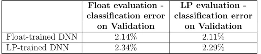
4.2.5 Mixing Training and Evaluation Types . . . 56
4.3 TIMIT . . . 57
4.3.1 Data, Task, and Model . . . 57
4.3.2 Smaller DNN . . . 58
4.3.3 Small Weight Updates . . . 59
4.3.4 Where Kahan Sums are Needed . . . 60
4.3.5 Full DNN . . . 62
4.4 WSJ . . . 63
4.4.1 Data, Task, and Model . . . 63
4.4.2 Smaller DNN . . . 64
4.4.3 Full DNN . . . 65
4.5 Even Less Precision . . . 67
4.6 Discussion . . . 68
5 Conclusion 71
B Additional Data 75
B.1 TIMIT Smaller DNN . . . 76
B.2 TIMIT Full DNN . . . 77
B.3 WSJ Smaller DNN . . . 78
List of Figures
2-1 A DNN with 2 hidden layers and an output layer [18]. Each hidden layer
typically has thousands of neurons, and the output layer has one neuron per
class. . . 20
2-2 An individual neuron [34]. The output of the neuron is the weighted sum
of its inputs plus a bias, passed through an activation function, such as the
sigmoid. . . 20
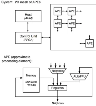
2-3 Bottom: A single LNS core, also known as an Approximate Processing
Ele-ment (APE). Top: A Singular chip consists of a grid of thousands of cores [11]. 28
2-4 One 25mm2 chip in the Singular prototype board from mid-2015. The board
has 16 chips, each with 2,112 cores [10]. . . 29
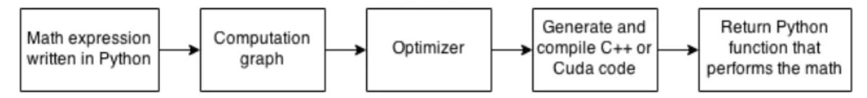
3-1 How Theano works: Theano converts the math expression into a Python
function that performs the computation. . . 38
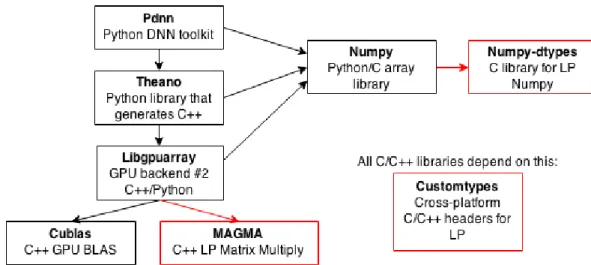
3-2 Architecture of the approximate DNN. Pdnn depends on Theano. Theano
itself has many dependencies. The red components are ones that we added.
LP was added to every component. . . 39
4-1 The MNIST task is to identify the digit in each image. . . 51
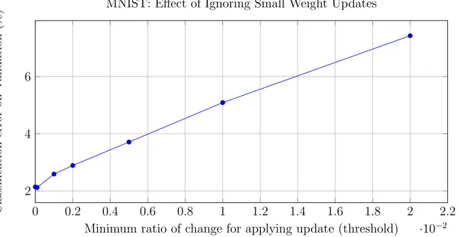
4-2 MNIST experiment to determine whether small updates to the weights can
be ignored in a float DNN. Weights updates are ignored if the absolute value
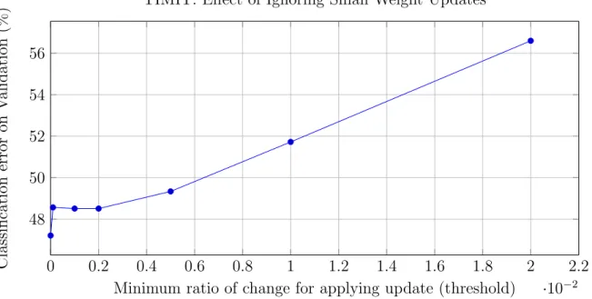
4-3 TIMIT experiment to determine whether small updates to the weights can be ignored in a 6x512 float DNN. Weights updates are ignored if the absolute
List of Tables
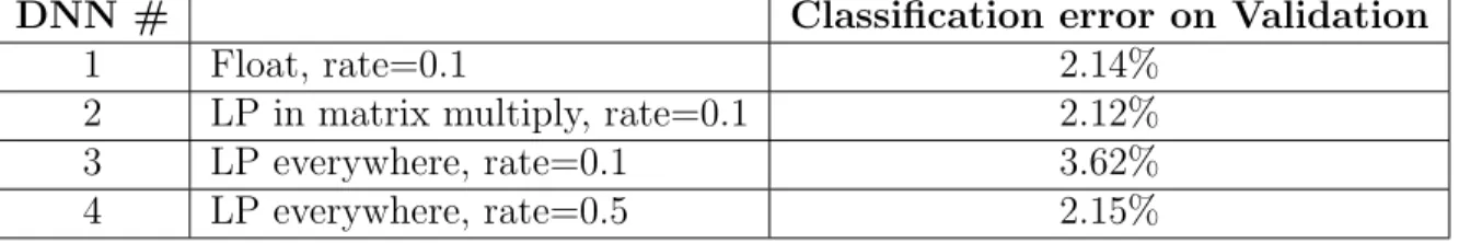
4.1 MNIST comparison of float DNN and approximate DNN. Kahan sums are
used only in the matrix multiply of the approximate DNNs. . . 53
4.2 MNIST comparison of float DNN and approximate DNN. Kahan sums are
used everywhere in the approximate DNN. . . 56
4.3 MNIST experiment that shows that a DNN can successfully be trained with
one datatype and evaluated with another. . . 56
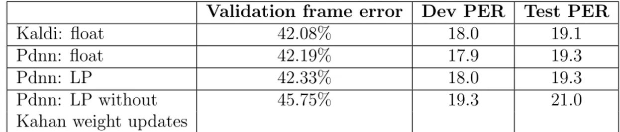
4.4 TIMIT comparison of smaller 6x512 float DNN and approximate DNN. The
first approximate DNN “Pdnn: LP” uses Kahan sums everywhere. The second approximate DNN “Pdnn: LP without Kahan weight updates” leaves out the
Kahan sum in the weight updates. . . 59
4.5 TIMIT experiment to determine where Kahan or pairwise sums are needed in
an approximate 6x512 DNN. DNNs with good results are highlighted in green. 61
4.6 TIMIT comparison of full-sized 6x1024 float DNN and approximate DNN. . 62
4.7 Experiment to determine how small a DNN and how much less data we could
use to get decent results on WSJ. The DNNs are all float-based. Bad results are highlighted in gray. We used the “7x512: 50% data” (yellow) for our
small-scale approximate DNN comparison. . . 64
4.8 WSJ comparison of smaller 7x512 float DNN and approximate DNN using
50% training data. . . 65
4.9 WSJ comparison of full-sized 6x2048 float DNN and approximate DNN using
4.10 Even lower-precision versions of LNS arithmetic. n is the number of bits in the fractional portion. Example computations are shown for 98 + 2 and 10 ∗ 10. 67
Chapter 1
Introduction
Machine learning is being used to solve problems that are increasingly important in day-to-day life. Machine learning techniques have been applied in fields such as bioinformatics, computer vision, economics, fraud detection, robotics, and speech. Recently, one of the most successful machine learning techniques has been Deep Neural Networks (DNNs). For instance, DNNs have currently been used extensively in the speech recognition community. For Automatic Speech Recognition (ASR), DNN-based models result in 10-30% relative improvement in word error rates over traditional methods [23]. Unfortunately, training a DNN is a time-consuming process, even when a graphics processing unit (GPU) is used to speed it up. In a speech task that uses 81 hours of speech as training data, the DNN takes more than half a day to train. It is general knowledge that speech recognizers benefit greatly from larger amounts of data; some systems use training sets with thousands of hours of speech. At the present rate, those DNNs would take weeks to train. Worse yet, selecting the best DNN architecture and tuning a DNN’s hyper-parameters typically require training many DNNs. The slow training is a significant impediment to DNN researchers.
Efforts to speed up the algorithm have focused on parallelizing the training algorithm, Stochastic Gradient Descent (SGD), to take advantage of more hardware. Chen et al. intro-duced pipelined SGD, which achieves 3.3x speedup with 4 GPUs. Unfortunately, speedup is limited by the number of layers in the network and the batch size, which must be reduced to
maintain the same error rates [16]. Google’s DistBelief system replicates a DNN across thou-sands of CPUs, training each with a subset of the data and periodically syncing the weights. Speedup is achieved for large DNNs with billions of weights, but not for moderately-sized DNNs used for speech [41]. Seide et al. achieved a speedup of 6.3 on a moderately-sized DNN by replicating the DNN on 8 GPUs and synchronizing the gradients. Communication is kept to a minimum with one-bit quantization of the gradients [40]. All these efforts have the drawback that they no longer use the original SGD training, but an approximation of it. They all required careful tuning to produce identical results to the SGD, and it is not clear whether they can always produce identical results. It seems that SGD can be sped up without modification only if the hardware gets faster.
One way to implement faster hardware is to use low-precision arithmetic. Certain algo-rithms can still produce good results even when using low-precision arithmetic. For those algorithms, the low-precision arithmetic is an acceptable trade-off for the faster computation afforded by the hardware. This thesis seeks to determine whether DNN training is one of those algorithms.
Although many types of low-precision arithmetic might exist, we focus our experiments on the arithmetic found in one particular hardware solution. Singular Computing, led by Joseph Bates, developed hardware that is 50 times faster per watt than a GPU. The Singular chip, as it is called, gains its speed by performing low-precision arithmetic, in which arithmetic operations produce values that are up to 1% away from the correct values. In this arithmetic, 98 + 2 = 99.776 and 10 ∗ 10 = 100.863. The precision is much lower than that of floating point arithmetic, which is traditionally used when training DNNs [11].
This thesis answers the following question: can a DNN based on low-precision arithmetic perform as well as a DNN based on floating point arithmetic? If the answer is yes, then low-precision hardware, such as the Singular chip, can be used to train DNNs faster without harming their ability to produce state-of-the-art results. We refer to DNNs that use low-precision arithmetic as “approximate DNNs” and DNNs that use traditional float-based arithmetic as “float DNNs.” This thesis makes the following contributions:
1. We add the low-precision arithmetic to a general-purpose math library that can be used to implement a variety of machine learning algorithms.
2. We implement an approximate DNN using the library.
3. We evaluate the approximate DNN on the TIMIT phoneme recognition task and the WSJ speech recognition task. For those tasks, we compare acoustic models based on approximate DNNs to ones based on float DNNs.
The evaluations show that an approximate DNN performs just as well as a float DNN. If Kahan summations are used, both types produce similar frame classification errors. When used as acoustic models in speech recognition, they generate near-identical recognition error rates. The low-precision arithmetic works, which means that the Singular chip can be used to speed up DNN training.
This thesis is organized as follows: Chapter 2 provides background on DNNs, speech recognition, the DNN speed problem, and the low-precision arithmetic solution to that prob-lem. Chapter 3 describes our implementation of the approximate DNN. Chapter 4 compares the approximate DNN to the float DNN on a small computer vision task (MNIST) and two larger speech recognition tasks (TIMIT and WSJ). Chapter 5 concludes.
Chapter 2
Background
This chapter provides background on Deep Neural Networks (DNNs) and the Stochastic Gra-dient Descent (SGD) training algorithm. We describe the use of DNNs in speech recognition and explain why training speed is an impediment to speech research. Existing approaches for speeding up DNN training are summarized. The low-precision hardware, which is another approach for speeding up training, is introduced. We describe the arithmetic used by the hardware and the software implementation of the arithmetic. The approximate DNNs that we evaluate are based on the low-precision arithmetic.
2.1
Deep Neural Networks
DNNs are used in classification tasks in which the goal is to assign one of C classes, or labels, to each input. The input is a feature vector that describes some observation. For example, in the MNIST classification task from machine vision, each input is a vector of pixel intensities taken from images of isolated handwritten digits. The classes are the digits 0-9, and the task is to predict the digit present in each image [29]. To solve classification tasks, we build a model, such as the DNN, that can estimate a posterior probability, P (class|input), for each class. For simple classification tasks, such as the digit identification problem described above, the predicted class for an input is simply the class with the highest posterior probability.
Figure 2-1: A DNN with 2 hidden layers and an output layer [18]. Each hidden layer typically has thousands of neurons, and the output layer has one neuron per class.
For a more complicated task, such as speech recognition, the posterior probabilities are used with other systems to solve the task.
Consider a DNN that has input x, which is the feature vector, and output y, which is the vector of class probabilities. The DNN consists of several hidden layers and an output layer. Each hidden layer typically has thousands of neurons. The output layer has C neurons, one for each class. An example DNN is shown in Figure 2-1.
Denote the output of each layer as yn, where n is the layer number. The first hidden
layer starts at n = 1. The output layer has n = N , where N is the number of layers in the
network. The input can be treated as a pseudo-layer: y0 = x. Each neuron has a weighted
connection from every output in the previous layer; there are no intra-layer connections. An example neuron is shown in Figure 2-2.
Figure 2-2: An individual neuron [34]. The output of the neuron is the weighted sum of its inputs plus a bias, passed through an activation function, such as the sigmoid.
The output of each neuron is a weighted sum of its inputs and a bias term, which is
passed through an activation function F . The output of each neuron in the nth layer, yn,j,
can be computed as:
yn,j = F ( X
i
(yn−1,i∗ wn,i,j) + bn,j) (2.1)
where neurons in layer n are indexed by j and neurons in layer n − 1 are indexed by i. The
weight from i to j is denoted by wn,i,j, and the bias of neuron j is denoted by bn,j. For
the hidden layers, common activation functions include the sigmoid, tangent, and rectifier functions. We use the sigmoid activation:
F (z) = 1
1 + e−z (2.2)
The output layer, also called the softmax layer, uses the softmax activation function:
F (zj) = ezj P
j
(ezj) (2.3)
Since the softmax normalizes yN to the range [0, 1] and ensures that it sums to 1, the outputs
can be treated as posterior probabilities.
It is believed that the power of a DNN comes from its depth. Layers closer to the input are able to learn low-level representations of the input, while layers further up are able to learn higher-level representations [24].
2.2
Training DNNs
The DNN is a highly non-convex model with multiple local optima; the most popular method of training one is Stochastic Gradient Descent (SGD). Using SGD, we train the DNN to minimize an objective function. Possible objective functions include cross-entropy and mean squared error. Variations of those functions also exist; some objectives have L1 and L2
regularization terms for example [33]. We use cross-entropy, which is computed as:
CEk = −
X
c
ln(yN,c,k) ∗ tc,k (2.4)
where the training example is indexed by k. The final layer’s output is denoted by the vector
yN,k, the classes are indexed by c, and tk is a vector of the one-hot encoded labels for that
example. SGD is a supervised training algorithm in which we train the network to predict labels of previously-labeled training data in the hope that the network will be able to predict labels for unlabeled data. The weights and biases of the DNN are first initialized; SGD then proceeds as shown in Algorithm 1 [12].
Algorithm 1 Stochastic Gradient Descent algorithm (one epoch) Shuffle the training dataset, and divide it into evenly-sized batches. for each batch of examples
Compute the DNN outputs, yN,k, with respect to the current weights and biases.
Compute the cross-entropy, CEk, for each example k.
for each layer n from N to 1
Compute the gradients dwn,i,jdCEk and dCEkdbn,j for each example k.
Sum the gradients across the examples to get one gradient per weight and bias: dCE dwn,i,j =X k dCEk dwn,i,j dCE dbn,j =X k dCEk dbn,j
Update each weight and bias according to the following formulas: wn,i,j0 = wn,i,j − α ∗ dCE dwn,i,j b0n,j = bn,j − α ∗ dCE dbn,j end for end for
Computing the outputs of the DNN is referred to as forward propagation since it involves using each layer’s output to compute the next layer’s output. Computing the gradients is
referred to as backpropagation since it involves propagating the error from the last layer back to the first layer. The interested reader can find the formulas for backpropagation in [33]. The process described above is repeated until the network converges. Each pass through the training set is an epoch. The parameter α, shown in Algorithm 1, is a learning rate that controls how much the network learns from each example; it is decreased as convergence slows. The method for setting and decreasing α is called a “learning rate schedule.” The convergence of the network is usually monitored on a held-out validation set.
The weights of a DNN can be initialized with random initialization or with pre-training. One of the possible ways to pre-train a DNN is by first training a stack of Restricted Boltz-mann Machines (RBMs). The RBM is a probabilistic graphical model. RBMs are stacked together and trained one layer at a time using greedy unsupervised training. Then, the weights of each RBM in the stack are used as the initial weights of the corresponding layer in the DNN. The interested reader can find details of the RBM training algorithm in [22].
During forward propagation, the training examples pass through the network layer-by-layer, with each node computing a dot product for each example. The dot products can be performed in parallel as a one matrix multiplication per layer. Backpropagation is similar computationally: there is one matrix multiplication per layer. The matrix multiplications dominate the runtime. They accounted for 85% of the runtime in one of our own GPU-based DNNs.
DNN training takes a long time for two reasons. First, SGD is a serial algorithm that processes examples batch-by-batch. The runtime is proportional to the amount of training data, and it typically takes dozens, and occasionally hundreds, of passes through the training data for the DNN to converge. Second, each batch of data causes 2N matrix multiplications, where N is the number of layers in the network. The matrix multiplications are slow since the matrices have dimensions equal to the number of units in each layer. The computations can be performed about 50 times faster on a GPU than on a CPU, but training is still slow even with the speedup.
2.3
Speech Recognition
Speech recognition is the task of converting speech audio to text. A speech recognizer consists of three parts: the acoustic model, the lexicon, and the language model. The acoustic model is a probabilistic model that describes which phonemes are likely to be present in a section of speech. The lexicon is a probabilistic model of which phonemes are used to pronounce a word. The language model describes the probabilities of different sequences of words. A related task is phoneme recognition, which aims to convert speech into a sequence of phonemes instead of a sequence of words. DNNs make effective acoustic models. Acoustic models based on a Hidden Markov Model (HMM) and DNN hybrid result in 10-30% relative improvement in word error rates over traditional methods, such as the HMM and Gaussian Mixture Model (GMM) [23]. For DNN-based acoustic models, the inputs are acoustic frames and the labels are phoneme states.
The slow training of DNNs is an impediment to speech research. For example, a DNN with 6 hidden layers of 2048 units, and an output layer of 3405 units, takes 50 minutes per epoch, and 16 epochs to converge, or approximately 13 hours total, on a GeForce GTX TITAN Black GPU. That DNN uses 81 hours of recorded speech from the Wall Street Journal corpus as training data [15], but much larger datasets exist. For example, [20] describes a dataset with 3,000 hours of recorded speech, and [26] describes a dataset with 5,780 hours of speech. Using more training data is desirable since it produces lower error rates, but standard SGD would take many weeks on a GPU for the larger datasets.
2.4
Existing Approaches for Faster Training
There are two main approaches to speed up DNN training. The first approach is to replicate the DNN across available hardware. In a naive implementation, the replicas start with iden-tical weights. Each replica processes a subset of the batch and computes its own gradients. The replicas synchronize by sending their gradients to a master replica. The master replica adds the gradients together to compute the weight updates and sends the new weights back to
every replica. Once every replica has updated, they all proceed to the next batch. Although the naive implementation is equivalent to true SGD, it does not work for two reasons. First, the communication cost of sending the gradients and weights is too high. Second, computing on small sub-batches is inefficient.
Google’s DistBelief system replicates the DNN across multiple machines. Instead of proceeding in lock-step, the replicas push their gradients and receive weight updates asyn-chronously. With 81 machines, a locally-connected DNN with 1.7 billion parameters achieves significant speedup. However, a moderately-sized, fully-connected DNN with 42 million pa-rameters achieves almost no speedup over the standard non-parallelized GPU-based SGD [17]. The moderately-sized DNN is the kind typically used in speech recognition.
Seide et al. replicate the DNN across multiple GPUs on a single machine. To lower the communication cost, their system compresses each gradient to a single bit using one-bit quantization. The compression is extremely lossy, so they use error feedback to ensure that all gradients are eventually accounted for. They achieve a speedup of 6.3-times on a moderately-sized DNN using 8 GPUs [40].
The second main approach is pipelining. Chen et al. pipeline the DNN by assigning layers to different GPUs. The GPUs are all kept busy by feeding in the next batch of examples before the current batch has finished. Pipelining requires smaller batch sizes to produce comparable error rates. With 4 GPUs, the pipelined system achieves a speedup of 3.3-times. Further scalability is limited by the number of layers and the reduction in batch size [16].
All these techniques have disadvantages. Some do not achieve speedup on speech DNNs. To maintain the same error rates, most require careful tuning and tricks, such as error feedback and smaller batch sizes. It is not always clear if these techniques can produce the same results as the true SGD algorithm. Faster hardware is likely the only way to speed up true SGD.
2.5
Low-Precision Hardware for Faster Training
Faster hardware can be implemented by using low-precision arithmetic. This type of hard-ware can speed up algorithms, but there is a trade-off. The low-precision arithmetic may worsen the algorithm’s results. The faster hardware is useful only if the algorithm is able to produce near state-of-the-art results when using low-precision arithmetic. In this thesis, we evaluate whether low-precision arithmetic can be used to train DNNs. Although different types of low-precision arithmetic might exist, we focus our evaluations on the low-precision arithmetic from one particular hardware solution: the Singular chip.
The Singular chip, developed by Joseph Bates of Singular Computing, is an alternative to the GPU that is 50 times faster per watt. The Singular chip can be used to speed up true SGD without resorting to modifying the algorithm. The parallelized variants of SGD might also benefit from being run on multiple Singular chips, but this thesis is concerned only with true SGD.
The Singular chip gains its speed by performing low-precision Logarithmic Number Sys-tem (LNS) arithmetic instead of the traditional based arithmetic. Traditional float-based arithmetic, such as the one defined by the IEEE-754 standard, is high precision and high dynamic range. IEEE floats have seven significant decimal digits of precision, which
means that the arithmetic results in values that are within a factor of 10−7 of the correct
values [27]. High dynamic range means that a wide range of values can be represented, such as the range of one billionth to one billion. In contrast, the LNS arithmetic used by the Singular chip is low precision and high dynamic range. A wide range of values is supported, but the arithmetic results in values that are 1% off from the correct values [11].
Conventional floats are represented as signif icand ∗ baseexponent. For example, 1.2345 is
represented as 12345 ∗ 10−4. The three parts of the float are stored in memory as a single
32-bit value [25]. In contrast, LNS represents a number as its base 2 logarithm. 1.2345
would be represented as log2(1.2345); the value of the logarithm is stored in memory using
a fixed-point representation. A fixed-point representation represents the value in binary, devoting a fixed number of bits to the integer portion of the number and a fixed number of
bits to the fractional portion [11].
The Singular chip uses 6 bits to represent the fractional part of a number’s logarithm. With 6 bits, increasing or decreasing the fractional part of the logarithm by 1 corresponds to
multiplying or dividing the number by 64√
2., which is approximately 1.011. Valid numbers in this system are therefore spaced apart by a factor 1.011. The gaps in the number line mean that numbers will be represented with a possible error of 1% from their true values. Singular uses 5 bits plus a sign bit to represent the integer part of the number’s logarithm. 5 bits is enough to represent logarithms from 0-31, meaning that a high dynamic range, with numbers from 0 to a billion, is representable [11].
Low-precision LNS can be implemented in hardware with far fewer physical resources. Conventional floating point arithmetic, particularly multiplication and division, require on the order of hundreds of thousands of transistors to implement. LNS arithmetic, on the other hand, is easier to implement in hardware. For instance, multiplication and division in LNS are implemented simply as addition and subtraction of the logarithms, which require fewer transistors. The number of arithmetic processing units, or cores, that fit on a chip is much higher with LNS than with float [11].
The Singular chip is implemented as a SIMD machine that performs parallel LNS oper-ations. When optimized and manufactured using the same process, a Singular core is 1% the size of a GPU core. This is the source of Singular’s 50x increase in compute speed, per watt or per area. Compute speed is also affected by memory bandwidth; Singular’s memory bandwidth can be 500 times that of a GPU [9]. The Singular design is shown in Figure 2-3. A prototype Singular board from mid-2015, shown in Figure 2-4, has 34,000 cores, per-forms 6 trillion operations per second (Tops), has 13 TB/s of memory bandwidth, and draws 50 watts [10, 9]. For comparison, a high-end commercial GPU has 3,000 cores, performs 5.1 Tops, has 0.3 TB/s of memory bandwidth, and draws 250 watts [38, 28]. In general, using the same silicon technology and with significant effort to optimize implementations, the Singular architecture shows about 50x better speed/power than GPUs [10]. A scaled-up version of the Singular chip (not the prototype) would speed up DNN training with true
Figure 2-3: Bottom: A single LNS core, also known as an Approximate Processing Element (APE). Top: A Singular chip consists of a grid of thousands of cores [11].
SGD. The question remains whether such a DNN would produce worse error rates due to the low-precision LNS.
Surprisingly, despite the low precision of the arithmetic, a variety of algorithms still
produce near state-of-the-art results when using LNS instead of floats. Example
algo-rithms include visual background subtraction via GMMs, stereo depth camera algoalgo-rithms, visual feature extraction and tracking, image manipulation using FFTs, and deblurring with Richardson-Lucy deconvolution [10].
Note that low-precision LNS is well-studied idea; other open implementations exist. One such implementation can be found in FloPoCo, an open-source VHDL library that can be used to implement LNS in hardware [1]. In general, the details of the LNS can vary. It can be implemented with analog or digital circuits, use more or less precision, and be implemented in any architecture, including SIMD, GPU, CPU, FPGA, and mobile [11]. The Singular chip is one instance of low-precision LNS hardware. This thesis determines whether DNNs based on low-precision arithmetic are also effective as acoustic models in speech recognition. We evaluate the arithmetic, not the hardware.
Figure 2-4: One 25mm2 chip in the Singular prototype board from mid-2015. The board has 16 chips, each with 2,112 cores [10].
2.6
Low-Precision Arithmetic
Although there are many types of low-precision (LP) arithmetic available, we used the one found in the Singular chip. Bates provided us with a software simulation of the Singular chip’s low-precision LNS arithmetic. The simulation is written in C, and we used it to implement the approximate DNN. The simulation includes: functions for converting between float and LNS; functions for multiplication, division, addition, subtraction, negation, and comparisons; and exponential and logarithm functions. LNS numbers are stored in the format shown in Listing 2.1.. | - - - l o g a r i t h m of n u m b e r - - - -| [ n u m b e r s i g n bit ][ s i g n bit ][ i n t e g e r p a r t (5 b i t s ) ][ f r a c t i o n p a r t (6 b i t s ) ] // As c o d e : s t r u c t g a _ u s e r t y p e 0 1 { int s i g n ; // n u m b e r s i g n bit
int val ; // l o g a r i t h m of number , s t o r e d as fixed - p o s i t i o n v a l u e
};
Listing 2.1: The LP type definition in C. The type stores the sign and logarithm of the number. The code refers to the LNS numbers as ‘ga usertype01.’
There is also a NaN bit, which is set on overflows and errors; we omit the overflow checks in all the example code for clarity.
a fixed-position value and also storing the sign of the float. Multiplication and division are implemented by adding and subtracting the logarithms and adjusting the signs as needed. Multiplication is shown below:
g a _ u s e r t y p e 0 1 u s e r t y p e 0 1 _ m u l t i p l y ( g a _ u s e r t y p e 0 1 a , g a _ u s e r t y p e 0 1 b ) { g a _ u s e r t y p e 0 1 r e s u l t ;
r e s u l t . s i g n = a . s i g n ^ b . s i g n ; r e s u l t . val = a . val + b . val ;
r e t u r n r e s u l t ; }
Addition and subtraction in LNS is more complicated. Consider two numbers B and C, represented as their logarithms, b and c. The result of adding B and C is represented by log(B + C), which can be computed with the following formula:
log(B + C) = log(B ∗ (1 + C/B)) = log(B) + log(1 + C/B) = b + G(c − b) (2.5)
where G(x) is the function, log(1 + 2x). To compute B + C, the addition function computes
c − b, feeds that through G, and adds the result to b [11]. There are many ways to compute G efficiently in hardware; Singular uses a proprietary method that is simulated in the C code. Subtraction works similarly.
The LNS exponential and natural logarithm functions are computed respectively with 4th and 5th order Taylor series approximations:
ex = 1 + x +x 2 2! + x3 3! + x4 4! (2.6) ln(x) = ln(1 + y 1 − y) = 2(y + y3 3 + y5 5 ) (2.7)
where y = x−1x+1. The interfaces of the C simulation functions are shown in Listing 2.2.1 The
LP operations of the simulation are about 10 times slower than their float equivalents since the simulation does not run on LP hardware.
1At this time, the full LP simulation is still proprietary. Those interested in using the code for research
// C o n v e r s i o n f u n c t i o n s : float - > LNS and LNS - > f l o a t g a _ u s e r t y p e 0 1 f l o a t _ t o _ u s e r t y p e 0 1 (f l o a t f ) ; f l o a t u s e r t y p e 0 1 _ t o _ f l o a t ( g a _ u s e r t y p e 0 1 x ) ; // LNS add , s u b t r a c t , m u l t i p l y , and d i v i d e g a _ u s e r t y p e 0 1 u s e r t y p e 0 1 _ a d d ( g a _ u s e r t y p e 0 1 x , g a _ u s e r t y p e 0 1 y ) ; g a _ u s e r t y p e 0 1 u s e r t y p e 0 1 _ s u b t r a c t ( g a _ u s e r t y p e 0 1 x , g a _ u s e r t y p e 0 1 y ) ; g a _ u s e r t y p e 0 1 u s e r t y p e 0 1 _ m u l t i p l y ( g a _ u s e r t y p e 0 1 x , g a _ u s e r t y p e 0 1 y ) ; g a _ u s e r t y p e 0 1 u s e r t y p e 0 1 _ d i v i d e ( g a _ u s e r t y p e 0 1 x , g a _ u s e r t y p e 0 1 y ) ; // LNS c o m p a r i s o n s int u s e r t y p e 0 1 _ e q ( g a _ u s e r t y p e 0 1 x , g a _ u s e r t y p e 0 1 y ) ; int u s e r t y p e 0 1 _ n e ( g a _ u s e r t y p e 0 1 x , g a _ u s e r t y p e 0 1 y ) ; int u s e r t y p e 0 1 _ l t ( g a _ u s e r t y p e 0 1 x , g a _ u s e r t y p e 0 1 y ) ; int u s e r t y p e 0 1 _ g t ( g a _ u s e r t y p e 0 1 x , g a _ u s e r t y p e 0 1 y ) ; int u s e r t y p e 0 1 _ l e ( g a _ u s e r t y p e 0 1 x , g a _ u s e r t y p e 0 1 y ) ; int u s e r t y p e 0 1 _ g e ( g a _ u s e r t y p e 0 1 x , g a _ u s e r t y p e 0 1 y ) ;
// LNS exp and n a t u r a l log ( u s i n g T a y l o r a p p r o x i m a t i o n s )
g a _ u s e r t y p e 0 1 u s e r t y p e 0 1 _ e x p ( g a _ u s e r t y p e 0 1 y ) ; g a _ u s e r t y p e 0 1 u s e r t y p e 0 1 _ l o g ( g a _ u s e r t y p e 0 1 y ) ;
Listing 2.2: Function interfaces of the C simulation provided by Bates. There are functions for converting between LNS and float and for performing LNS arithmetic.
2.6.1
Kahan Sums
One of the negative effects of low-precision LNS arithmetic is that in-place additions, such as A += B, produce no change in A if B is much smaller than A. Since valid numbers in this system are spaced apart by a factor 1.011, the only way for the addition to change A is if B is large enough to push A to the next valid value. B must be more than about 1% of A. This effect causes problems when summing many numbers. Once the total grows large enough, the remaining numbers in the sum do not get added to the total. For example, adding 1000 ones in LNS produces a wildly inaccurate value of 179.069.
t o t a l = LNS (0)
for i in x r a n g e( 1 0 0 0 ) : t o t a l += LNS (1)
p r i n t t o t a l # 1 7 9 . 0 6 9 3 9 7
Once the sum gets above 179.069, the remaining ones in the sum are too small to change the total. Note that conventional float arithmetic also has the same problem, but the problem
occurs only in more extreme cases. With seven significant decimal digits, float sums fail
only when B < 10−7 ∗ A instead of when B < 10−2 ∗ A. Adding 1000 ones is one of the
non-extreme cases; the float arithmetic produces the expected result of 1000:
t o t a l = f l o a t(0)
for i in x r a n g e( 1 0 0 0 ) : t o t a l += f l o a t(1)
p r i n t t o t a l # 1 0 0 0
Bates found that the Kahan summation algorithm can solve the inaccuracy in linear sums of LNS numbers. The algorithm works by keeping a running compensation of the accumulated error in the total. The error is added back to the total on each iteration of the sum. Kahan is implemented by adding an extra variable to hold the compensation and by replacing the addition operation with 2 additions and 2 subtractions [21]. As shown below, Kahan produces a decent result of 991.263, which is within 1% of the correct result.
t o t a l = LNS (0) c o m p e n s a t i o n = LNS (0) for i in x r a n g e( 1 0 0 0 ) : tmp = c o m p e n s a t i o n + LNS (1) n e w t o t a l = t o t a l + tmp c o m p e n s a t i o n = tmp - ( n e w t o t a l - t o t a l ) t o t a l = n e w t o t a l p r i n t t o t a l # 9 9 1 . 2 6 3 6 1 1
The Kahan sum bounds the error to O(1). An alternative solution is to sum the LNS numbers pairwise. Pairwise addition uses divide-and-conquer to add pairs of numbers at a time, and it bounds the error to O(logN ) [21]. As shown below, pairwise summation of 1000 ones in LNS produces a better result of 1002.058.
def p a i r w i s e ( n ) : if n == 0: r e t u r n LNS (0) if n == 1: r e t u r n LNS (1) mid = n /2 r e t u r n p a i r w i s e ( mid ) + p a i r w i s e ( n - mid ) t o t a l = p a i r w i s e ( 1 0 0 0 ) p r i n t t o t a l # 1 0 0 2 . 0 5 7 8 0 0
It turns out that an LNS-based DNN cannot perform as well as a float-based DNN unless Kahan or pairwise sums are used to maintain precision in certain sums.
2.7
Summary
The SGD algorithm used to train DNNs is slow, especially when the training dataset is large. Existing approaches to speed up SGD all involve significant modification to the algorithm. Since the variations of the algorithm work differently, we cannot expect them to produce the same results as SGD every time. The only way to speed up the true SGD algorithm is with faster hardware. Low-precision hardware, such as the Singular chip, is faster than existing GPUs but performs only low-precision arithmetic. This thesis determines whether a DNN can be trained using low-precision arithmetic to produce state-of-the-art results. The rest of this thesis refers to low-precision arithmetic as LP arithmetic and any type of hardware that uses it as LP hardware.
Chapter 3
Implementation of Approximate DNN
Most DNN toolkits, including the one we use as a baseline, are based on IEEE-754 float. To implement the approximate DNN, we added the low-precision (LP) type to an existing DNN toolkit. We then trained approximate DNNs as acoustic models for speech recognition and compared them to DNNs trained using IEEE-754 float. The approximate DNNs take much longer to train because they are based on the slow LP arithmetic simulation. Training time is not an issue since we only care about whether the approximate DNN will converge. Training will be faster once it implemented on LP hardware, but we only evaluate the LP arithmetic for now.
The DNN toolkit we selected for our experiments was Pdnn [32]. Pdnn is written in Python, and it uses the Theano library for all its computations. Theano is a Python library
for general-purpose math [8, 13]. It allows users to define and evaluate mathematical
expressions involving arrays and tensors with very few lines of high-level code. Behind the scenes, Theano compiles the mathematical expressions into C++ code, which can execute either on the CPU or the GPU. Adding the LP type to Pdnn requires adding it to the Theano library. The main advantage of using Theano is that we can quickly change and test our approximate DNN. In addition, by adding LP to Theano, we also get a LP library that can be used to implement other non-DNN algorithms.
IEEE-754 float DNN, which it uses to build acoustic models. (Kaldi actually has two DNNs; this thesis only considers the “Karel DNN” version). For our experiments, we treat the Kaldi DNN as the state-of-the-art baseline. We modify Pdnn so that it can be switched in as a replacement for the Kaldi DNN. We train acoustic models using the Kaldi DNN, the Pdnn float DNN, and the Pdnn approximate DNN and compare the word error rates achieved by the three. The rest of this chapter describes how we add LP to Pdnn and Theano.
3.1
Pdnn
Our first task was to make sure that Pdnn could achieve state-of-the-art results comparable to Kaldi DNN. The Pdnn website reports that an acoustic model built with Pdnn DNN achieves a dev set phoneme error rate (PER) of 18.8% and a test set PER of 20.2% on the TIMIT phoneme recognition task [31]. These results, which we reproduced, are worse than the 17.5% dev set PER and 18.5% test set PER reported for Kaldi DNN [39]. It would not make sense to use Pdnn for our experiments if it could not match the results of the Kaldi DNN. Therefore, we changed Pdnn to match the Kaldi DNN results.
Pdnn differs from Kaldi DNN in several ways. Pdnn performs its own feature processing and label alignment using Kaldi’s scripts. It converts the features and labels into non-Kaldi storage format. Pdnn also has different weight initialization. The random initialization of Pdnn draws from slightly different distributions, and RBM-based initialization uses Pdnn’s own implementation of RBM. Pdnn also trains the network using an exponentially decaying learning rate, which differs from the learning rate schedule of Kaldi DNN. Kaldi’s schedule can be found in the experiment of Section 4.3.2. Finally, it performs its own posterior extraction and decoding using Kaldi’s scripts.
We eliminated those differences to make Pdnn perform as well as Kaldi DNN. Pdnn now uses the same features and label alignments as the Kaldi DNN; it loads the features and labels using a Python port of the C++ Kaldi data loader. To port the Kaldi data loader, we wrote a C wrapper for the necessary C++ classes and exposed the wrapper to Python using the Ctypes (C-to-Python) library. We also wrote a model loader that could initialize Pdnn
using either Kaldi-initialized DNNs or Kaldi-trained RBMs. We replaced the exponentially decaying learning rate in Pdnn with the Kaldi DNN learning rate schedule. Finally, we made sure that Pdnn extracted posteriors and decoded in the same way as Kaldi DNN. With these changes, Pdnn produces error rates that are very close to those of Kaldi DNN. Pdnn is suitable for our experiments since Pdnn and Kaldi DNN can be now be compared in an apples-to-apples comparison.
3.2
Theano
In this section, we present background on Theano and describe its architecture. Then we describe how we add LP to each component of Theano’s software stack. This section assumes basic knowledge C, C++, and Python. We first introduce additional programming concepts needed for understanding Theano.
3.2.1
Background
Theano is made up of several libraries. The libraries are a mix of Python, C, C++, and Cuda code. Cuda is a variant of C++ that runs on Nvidia GPUs [37]. In Cuda, functions are declared as either “host” functions that run on the CPU, or as “device” functions that run on the GPU. Host and device functions are the same, except that host functions must access host memory and device functions must access device memory. Cuda code also has kernels, which are another type of device function. Cuda is compiled with its own compiler (nvcc). There are associated Cuda libraries, such as the Cublas library that performs linear algebra and matrix math [37].
Many of the libraries are for Python. Python modules and classes are usually written in Python, but they can also be written in C/C++. The modules and classes written in C/C++ are referred to as Python Extensions [6]. Python Extensions are compiled into shared objects that can be dynamically loaded by Python. Both Cuda and Python Extensions are used frequently in Theano.
3.2.2
Architecture
Theano allows users to build mathematical expressions involving symbolic variables in Python. For example, a Theano expression for a DNN hidden layer can simply be written as:
layer_output = T.sigmoid(T.dot(layer_input, weights) + biases)
where layer output, layer input, weights, and biases are Theano variables that represent arrays and vectors. The user compiles the expression, specifying which variables are inputs and which variables are outputs. The result of compilation is a callable Python function that performs the computation. When compiling an expression, Theano internally creates a computation graph, where nodes are operations and variables. Theano’s optimizer then applies optimizations to the graph. The optimizations speed up the computation by simplifying the expression, reducing memory usage, reducing data transfers, and, if a GPU is available, promoting operations from the CPU to the GPU.
Finally, Theano generates C++ code for each operation. The C++ code for each oper-ation is saved onto the filesystem and compiled into a Python Extension using the system’s C++ compiler. Instead of C++, Cuda code is generated for operations that execute on the GPU; it is compiled with the Cuda compiler. Theano then returns a function that, when called, executes the entire computation graph by loading each Python Extension and exe-cuting each operation. Some operations do not have C++ or GPU equivalents yet; those instead execute directly in Python. All the compiled C++ and Cuda code is cached to avoid unnecessary re-compiling. The entire process is summarized in Figure 3-1.
Figure 3-1: How Theano works: Theano converts the math expression into a Python function that performs the computation.
Pdnn depends on Theano. Theano generates the C++ code by itself and depends on a GPU backend to generate the Cuda code. There are two possible GPU backends. The
first GPU backend, “sandbox.cuda,” is included with Theano. The second GPU backend, Libgpuarray [3], is an external component. We chose to use the second GPU backend, Libgpuarray, for our approximate DNN. The GPU backend depends on the Cublas library to perform some matrix operations, such as matrix multiply. All the components, except for Cublas, depend on Numpy to manipulate arrays in Python [5]. The Theano stack is shown in Figure 3-2.
Figure 3-2: Architecture of the approximate DNN. Pdnn depends on Theano. Theano itself has many dependencies. The red components are ones that we added. LP was added to every component.
To add LP to Pdnn-Theano, we add three components to this stack. Our additions are pictured in red in Figure 3-2. The first addition is Customtypes, a library that contains the LP simulation code in one place for all the other components to use. The second addition is Numpy-dtypes [14], a library that allows us to add user-defined types to Numpy. The third addition is Magma, an open-source version of Cublas that we use to write LP matrix multiplication [4].
We added LP to the stack one component at a time, making sure to observe the depen-dencies so that we could test each component before moving on to the next. LP was added to components in this order: Customtypes, Numpy-dtypes, Magma, Libgpuarray, and Theano.
3.2.3
Customtypes
The C simulation code provided by Bates is needed by nearly every component. It is used by the C code in Numpy-dtypes and Libgpuarray and the Cuda code in Magma. Theano generates C++ and Cuda code that also uses it. Since all the components need it, we implemented the Customtypes library to provide a version of the simulation that works in C, C++, and Cuda.
Customtypes has a single header file with all the code for LP. We chose not to compile the LP code into a static or shared library since linking against it caused runtime errors in Cuda. Instead, the other components include the header wherever they need it. The header depends on compiler macros for cross-device and cross-language compatibility. If the C compiler is detected, the header defines the LP struct and C functions that operate on it. If the C++ compiler is detected, the header defines a LP struct with C++ methods, the C functions, and overloaded versions of built-in C++ arithmetic functions and operators. If the Cuda compiler is detected, the header behaves as if the C++ compiler was detected, but it also declares all the methods, functions, and operators to be executable on both host and device. Finally, we use Cuda macros to generate different versions of the functions when necessary: host functions access host global variables and call host-only functions, while device functions access device variables. A snippet of the header file is shown in Listing A.1 of Appendix A.
Theano normally generates C++ and Cuda code only for floats and other built-in types. That code uses built-in C++ operators (e.g. +, -, /, *) and functions (e.g. max and abs). Since we overloaded all those operators and functions for LP, most of the generated code that works for floats also works for LP. We did not need to change code generation for it to work with LP.
The LP struct has a constructor that allows for float-to-LP casts. We made sure not to define a LP-to-float cast using a user-defined conversion [7]. Omitting LP-to-float ensures that C++ uses the LP arithmetic. In C++, operations on variables of two different types will promote one of the types as necessary. For example, when adding a float and integer, the
integer is promoted to a float, and float addition is performed. By overloading the built-in operators, we enabled operations between LP and float. By omitting LP-to-float casts, we ensure that those operations will promote float to LP and perform LP arithmetic instead of promoting LP to float and performing float arithmetic. If Theano generates any code that violates these conditions, the compiler will fail, and we can easily identify and fix the offending code. In addition, by leaving out LP-to-float casts, there is no way to store an LP result in a float without using a specific function that we wrote. The function is easy to search for in the source code, so it is easy to verify that the generated code performs only LP arithmetic on LP variables. These techniques guarantee that once a number has been converted to LP, it stays in LP unless explicitly converted to float. The operators and functions were overloaded in such a way that operations involving at least one LP operand use LP arithmetic and produce an LP result.
3.2.4
Numpy
The next component was Numpy, the standard library used for performing numerical op-erations on Python arrays. The Numpy-dtypes library provides an example of adding a user-defined type to Python and Numpy. Following that example, we added LP to Numpy-dtypes.
The LP version of Numpy-dtypes is a Python Extension written in C. To define a LP type that can be manipulated in Python, we registered the LP struct and C implementations of a class constructor, getters, setters, casts, string representation, and serialization functions using Python’s C API. We also registered the LP arithmetic functions. We then added the LP type to Numpy by registering the arithmetic functions using Numpy’s C API. The two APIs set a few variables in the Python extension. Theano requires access to them, so we used the Python Capsules API to export the variables. The LP struct and arithmetic functions came from the C section of the LP header in Customtypes.
Finally, we made two changes to the Numpy library itself. The first change fixed a bug related to user types. Numpy allows user-defined types to be stored in memory either
as a struct or as a pointer to a struct, but part of it incorrectly assumes only the latter. The second change deals specifically with LP. The value of zero in LP is not represented in memory by a zero. However, Numpy wrongly assumes that the value of zero for all data types is represented by zero in memory, and it uses C’s calloc() function to clear the memory when creating arrays of LP zeros. We changed Numpy so that it uses Python to assign LP zeros instead of using C to clear the memory.
With Numpy-dtypes, we can instantiate and manipulate LP values in Python or Numpy just like any built-in data type.
3.2.5
Magma
The Theano GPU backend depends on Cublas for many array operations, including matrix multiply. To implement LP matrix multiply on the GPU, we used Magma, an open-source alternative to Cublas, as a starting point. We only implemented the LP matrix multiply in Magma since the other operations are not used by Pdnn.
Magma contains matrix multiplies for float, double, single precision complex, and double precision complex numbers. Each type’s matrix multiply includes: (1) data type struct declaration, (2) definition of add, subtract, multiply, and convert-from-float functions, (3) a function for fetching the data type from device memory, and (4) several kernels and header files that define the matrix multiply for that type. We copied the float matrix multiply code and replaced the appropriate definitions to change it into a LP matrix multiply. We then changed the LP matrix multiply to a Kahan matrix multiply: the dot products inside the matrix multiply use Kahan summations.
Magma is the one component of our Theano stack that does not use Customtypes directly. Because the performance of matrix multiply is critical to the speed of the DNN, we needed to optimize the LP data type specifically for matrix multiply. We copied the LP add, subtract, and multiply code into Magma and experimented with it to increase the speed of LP matrix multiply. We tried rewriting the LP functions to be as simple as possible and varying the thread block sizes.
With Kahan matrix multiply of LP, the best performance we ever achieved when multi-plying two 2048x2048 matrices was 40 Gops, or billion operations per second. In contrast, Cublas float matrix multiply on the same-sized matrices achieves 3000 Gops. Despite the difference, the 100x slowdown is not unexpected, according to our benchmarks. Magma’s matrix multiply, on which we based the LP version, achieves 1500 Gops, or half the speed of Cublas. If you change the float into a struct containing a float, which is similar to the LP definition, Magma’s performance halves to 750 Gops. Adding Kahan further reduces performance by a factor of 2.5 to 300 Gops since the two operations in the dot products (add and multiply) turn into five operations (two adds and two subtracts from Kahan and one multiply). If you account for the fact that each of the LP simulation operations takes around 10 times as many steps, reducing the float performance to 30 Gops is reasonable, and this estimate is close to what our LP Kahan matrix multiply achieves. In practice, our approximate DNNs were 10-30 times slower than the float DNNs.
3.2.6
Libgpuarray
Theano includes two GPU backends. Theano uses the backend to generate Cuda code and to execute GPU operations. The first backend, “cuda.sandbox,” is the default included with Theano. It only supported operations on 32-bit floats; selecting another type causes Theano to fall back to CPU execution. The second backend, Libgpuarray, supported GPU execution with 32-bit floats and 64-bit floats. Although other types would cause Theano to fall back to CPU execution, Libgpuarray already had partial support for other types (characters, integers, complex numbers, unsigned, and signed) that Theano was not taking advantage of. For that reason, we chose to add LP to Libgpuarray instead of “cuda.sandbox.”
Libgpuarray is made of a C library and a Python library. The C library is a utility library for GPU programming; it defines functions for GPU initialization, memory management, compilation and execution of kernels passed in as strings, array manipulation, and Cublas execution. The Python library depends on the utilities in the C library; it defines a Python class for a GPU array and functions for compiling and executing kernels. Theano uses the
Python class and functions.
To add LP to Libgpuarray, we searched the code for all instances of ‘complex’ or ‘cfloat’ (the name of the struct for complex numbers) and added corresponding code for LP. Both the C library and the kernels generated by the Python library used the LP code from Cus-tomtypes. We changed the C library so that the matrix multiply of non-LP continues to rely on Cublas, but the LP matrix multiply uses our LP Kahan matrix multiply from Magma.
One interesting part of the implementation was in the array copy. Libgpuarray has a function that copies from one GPU array to another. The source and destination of the copy each have one of over a dozen types. If you wrote a Cuda kernel to perform each copy,
there would be N2, or over a hundred, kernels in the source code. To avoid this problem,
Libgpuarray dynamically generates a kernel for each source and destination type as they are needed during runtime and uses Cuda to compile, load, and execute the kernel. To speed up the kernel compilation, Libgpuarray generates the kernel in Cuda Assembly instead of Cuda C++.
Unfortunately, assembly code for the LP type is hard to write, so we changed Libgpuarray to generate the kernel for LP array copy in Cuda C++. Compiling this kernel each time it is used turned out to be much slower since Cuda C++ takes much longer to compile than Cuda Assembly. Instead, we decided to avoid kernel generation for LP array copies. We wrote float-to-LP, LP-to-LP, and LP-to-float versions of the array copy kernel in Cuda C++ and compiled those with the rest of the source code instead of using the slower dynamic kernel generation and compilation. We did not support array copies from non-float types to LP or from LP to non-float types, otherwise we would have needed to write dozens of such kernels. However, if such copies are needed, the user can use a float array as an intermediary.
3.2.7
Theano and Pdnn
At this point, all of Theano’s dependencies had LP. The final step was to add LP to Theano and to make Pdnn use it. To make Pdnn use LP, we had to make sure that all its Theano vari-ables were created with type LP. Fortunately, Pdnn already created most its Theano varivari-ables
with type ‘theano.config.floatX.’ ‘theano.config.floatX’ is a user-configurable setting in Theano that is typically set to 32-bit float and occasionally 64-bit float. By making sure all Theano variables in Pdnn were created with type ‘theano.config.floatX’ and then adding LP to the list of permissible floatX types, we made it so that Pdnn could run with either 32-bit float or LP depending on this setting. When Pdnn is configured to use LP, float is only used for feature I/O and for saving the DNN; all computations are LP.
With Pdnn using LP, the last step was to add LP to Theano. To add LP to Theano, we took the approach of running Pdnn and looking for failures caused by operations that did not support the LP type. There are too many operations in Theano, and Pdnn only uses a small subset. This approach allowed us to add LP where it was needed more quickly. Often, the failure was caused by an operation asserting that its operands were 32-bit or 64-bit float. For these operations, we simply added LP to the list of permissible types. Theano included a few tables for defining data types; we added LP to those, again finding the tables by looking for table lookup errors when running Pdnn. We also changed the C++ code generation to include our Customtypes LP header file.
Theano operations can run as Python on the CPU, C++ on the CPU, or Cuda on the GPU. Most operations are added to the computation graph as Python operations; the Theano optimizer then examines the computation graph and promotes Python operations to C++ and C++ operations to GPU operations. The optimizer had type assertions that prevented the LP operations from being promoted to either C++ or GPU. We added LP to the permissible types in those assertions so that all LP operations would be promoted to C++ or, when possible, the GPU.
Finally, we ran the LP Pdnn on the MNIST task and fixed any errors that prevented
it from converging. Two of the errors dealt with overflows in LP. We changed the LP
exponential function to return 0 for inputs less than −20. We also changed the LP logarithm
function to return a large negative value (−108) for an input of 0. As a final optimization,
we rewrote the Theano GPU softmax operation to use more parallelism. For our TIMIT experiments, this halved the training time when using LP. This completes the implementation
of the basic approximate DNN.
3.3
Kahan Summation
With the approximate DNN completed, the next step was to add Kahan sums. Kahan sums turn out to be critical for the approximate DNN to match the float DNN. In Chapter 4, we analyze the importance of the Kahan sums. In this section, we describe how we add it to Theano and Pdnn.
In Theano and Pdnn, four of the operations that we use have linear sums: (1) Theano (Libgpuarray) matrix multiply, (2) Theano tensor sum, (3) Theano softmax, and (4) Pdnn weight updates. The tensor sum is used when summing the gradients for all the examples in a batch to get a single gradient for each weight and bias. We modified the four operations so that they use Kahan when operating on LP. Adding Kahan to the matrix multiply, tensor sum, and softmax is fairly straightforward since that mostly involves changing C++ code. Adding Kahan to the Pdnn weight updates is trickier.
Weight updates are a target for Kahan summation because they are a linear sum. During training, the gradient multiplied by the learning rate is added to each weight on each batch. There are thousands of batches per epoch and dozens of epochs. The gradients are usually much smaller than the weights that they are added to. Thus, weight updates are extremely long linear sums where very small numbers are being added to comparatively very large numbers. Weight updates are therefore an excellent candidate for Kahan sums. In Theano, the non-Kahan weight update is implemented as follows:
n e w _ w e i g h t s = T . add ( weights , u p d a t e s )
Kahan of the weight updates requires a compensation variable for every weight. For every weight matrix and bias vector in Pdnn, we create a separate matrix or vector of compensations. An obvious way to implement Kahan would then be to use the Theano add and subtract operations on each pair of weight and compensation arrays exactly as the Kahan algorithm is specified:
tmp = T . add ( c o m p e n s a t i o n s , u p d a t e s ) n e w _ w e i g h t s = T . add ( weights , tmp )
n e w _ c o m p e n s a t i o n s = T . sub ( tmp , T . sub ( n e w _ w e i g h t s , w e i g h t s ) )
This method does not work; it turns out to have the same effect as the non-Kahan update. The problem is caused by an aggressive optimizer. An aggressive optimizer will optimize away the Kahan sum if it applies the associative rule and simplifies the resulting expression [19]. This is true of optimizers in certain programming language compilers and of the Theano optimizer. Fortunately, the C, C++, and Cuda compilers do not apply the optimization, so our Kahan sums in the C++ code work as expected. Unfortunately, the Theano optimizer that analyzes the computation graph does apply the rules of associativity to associative operations, such as addition. To prevent the Theano optimizer from optimiz-ing away our Kahan sum, we copied the Theano tensor ‘add’ operation and declared that this new operation was not associative. Our new operation is named ‘add no assoc,’ and using it to implement Kahan prevented Theano from optimizing away the Kahan. The final implementation of Kahan weight updates is shown below:
tmp = T . a d d _ n o _ a s s o c ( c o m p e n s a t i o n s , u p d a t e s ) n e w _ w e i g h t s = T . a d d _ n o _ a s s o c ( weights , tmp )
n e w _ c o m p e n s a t i o n s = T . sub ( tmp , T . sub ( n e w _ w e i g h t s , w e i g h t s ) )
3.4
Verification
It is critical that we verify that the approximate DNN performs all computations with LP and not float. The slow execution of the approximate DNN is one indicator that we are performing LP computations since the LP simulation is slower than floats. However, to be absolutely sure, we verified our approximate DNN in two ways.
First, we printed the Theano computation graph for the training function of the approx-imate DNN. The resulting image displays all the Theano operations and their input and output types. If the computations in the DNN are performed with LP, then there should be
no values with floats. We found 5 values with floats, but they were acceptable since they are not involved in any arithmetic used by the training.
Our second verification method was to examine the C++ and Cuda code generated by Theano. For our approximate DNN, Theano generated 46 C++ and Cuda files; each file implements one operation. Libgpuarray also generates 5 Cuda files. We examined every source file to check that all arithmetic operations were performed with at least one LP operand and without typecasting that LP operand to float. After doing so, we know that all C++ and Cuda Theano operations used by Pdnn perform LP-only arithmetic. The only remaining place where float arithmetic might hide is in Python operations. It is harder to reason about the arithmetic performed by Python since Python is a dynamically typed language that will cast variables as needed. However, we ran Theano in ‘profile mode’ to print every operation and its method of execution. We confirmed that all operations had been promoted to either C++ or Cuda, which means no operations were running in Python. Thus, we concluded that no float arithmetic is performed in the approximate DNN.
3.5
Summary
Our final approximate DNN system is implemented in Pdnn. With one configuration change, we can run Pdnn as an approximate DNN or as a float DNN. We made sure that Pdnn could reproduce the state-of-the-art results achieved by the Kaldi DNN before converting it to an approximate DNN. To implement the approximate DNN, we added LP to the Theano math library used by Pdnn, which required adding LP to every component in the Theano software stack. Finally, we added Kahan summation to the LP versions of matrix multiply, tensor sum, softmax, and Pdnn weight updates. We verified that LP arithmetic was used in the approximate DNN instead of float arithmetic. In the next chapter, we describe experiments that compare the performance of a float DNN to that of an approximate DNN.
Chapter 4
Approximate DNN Experiments
In the this chapter, we evaluate the approximate DNN on three tasks - MNIST, TIMIT, and WSJ - to determine if it can do as well as a conventional float DNN. MNIST is a computer vision task, and TIMIT and WSJ are speech tasks. The tasks get progressively larger. MNIST, the smallest, has 50,000 training examples. TIMIT has 1,000,000 training examples. WSJ, the largest task, has 26,000,000 training examples. For all three tasks, we train approximate Pdnn and float Pdnn, using the same setup for both. We compare the classification error rates achieved by the two DNNs. For the two speech tasks, we also include the state-of-the-art Kaldi DNN results for comparison.
Although our changes to Pdnn should give float Pdnn similar performance to Kaldi DNN, we include both to give a complete comparison. Kaldi DNN still performs marginally better than float Pdnn, and therefore LP Pdnn. However, the difference is small enough that they can all be compared fairly. For speech tasks, we also compare an additional metric. With Kaldi, we build speech recognizers using the approximate Pdnn, float Pdnn, and Kaldi DNN. We compare the error rate achieved by the entire recognizer system, in addition to the DNN classification error rates. The approximate DNNs take longer to train since they use the slower LP simulation instead of faster LP hardware. We do not care about the training times because our experiments determine only whether the approximate DNN converges. All DNNs were trained on a GeForce GTX TITAN Black GPU using Cuda 6.0.
![Figure 2-1: A DNN with 2 hidden layers and an output layer [18]. Each hidden layer typically has thousands of neurons, and the output layer has one neuron per class.](https://thumb-eu.123doks.com/thumbv2/123doknet/13835355.443586/20.918.301.616.107.284/figure-hidden-layers-output-hidden-typically-thousands-neurons.webp)
![Figure 2-4: One 25mm 2 chip in the Singular prototype board from mid-2015. The board has 16 chips, each with 2,112 cores [10].](https://thumb-eu.123doks.com/thumbv2/123doknet/13835355.443586/29.918.352.568.107.346/figure-chip-singular-prototype-board-board-chips-cores.webp)