Acoustic source localization

Acoustic Source Localization

by

Nilu Zhao

B.S., Massachusetts Institute of Technology (2014)

Submitted to the Department of Mechanical Engineering

in partial fulfillment of the requirements for the degree of

Master of Science in Mechanical Engineering

at

_{JUN 0 2 2016}

MASSACHUSETTS INSTITUTE OF TECHNOLOGY

_LIBRARIES

June 2016

ARCHIVES

Massachusetts Institute of Technology 2016. All rights reserved.

Author.

Signature redacted...

Department of Mechanical Engineering

May

7, 2016

Certified by

Signature redacted

...

George Barbastathis

Professor

Thesis Supervisor

Signature redacted

Accepted by...

Rohan Abeyaratne

Chairman, Department Committee on Graduate Theses

Acoustic Source Localization

by

Nilu Zhao

Submitted to the Department of Mechanical Engineering on May 7, 2016, in partial fulfillment of the

requirements for the degree of

Master of Science in Mechanical Engineering

Abstract

Many technologies rely on underwater acoustics. Most of these applications are able to denoise Gaussian noise from the surrounding, but have trouble removing impulse-like noises. One source of impulse-impulse-like noise is the snapping shrimps. The acoustic signals they emit from snapping their claws hinder technologies, but can also be used as a source of ambient noise illumination due to the rough uniformity in their spatial distribution. Understanding the spatial distributions of these acoustic signals can be useful in working to mitigate or amplify their effects.

Our collaborators in Singapore use a multi-array sensor to take measurements of the sound pressures of the environment in the ocean. This thesis investigates in solving the signal reconstruction problem - given the measurements, reconstruct the locations of the orignal signal sources. A numerical model for the system consisting of the snapping shrimp signals, the environment, and the sensor is formulated. Three methods of recon-struction - Disciplined Convex Programming, Orthogonal Matching Pursuit, and Com-pressive Sensing- are explored, and their robustness to noise, and sparsity are examined

in simulation. Results show that Two-Step Iterative Shrinkage Threshold (TwIST) is the most robust to noisy and non-sparse signals. The three methods were then tested on real data set, in which OMP and TwIST showed promising consistency in their results, while CVX was unable to converge. Since there is no available information on ground truth, the consistency is a promising result.

Thesis Supervisor: George Barbastathis Title: Professor

Acknowledgments

First and foremost, I would like to thank my advisor, Professor George Barbastathis. He has guided me on my research since I was an undergraduate at MIT. I am extremely appreciative of his guidance -he has taught me the ways of research and given me much helpful advice.

I would like to thank our collaborators in the National University of Singapore,

Pro-fessor Mandar Chitre, and Too Yuen Min in their help on the development of the forward model, the acoustic data for the shrimps, and discussions on the project.

I am thankful for Yi Liu, for her mentorship and help on research; Wensheng Chen,

for his helpful suggestions and discussions on the project. I am also grateful for the rest of my labmates: Shuai Li, Kelli Xu, Adam Pan, Justin Lee, and past labmates Yunhui Zhu, Max Hsieh, Jeong-gil Kim, for their help and many good memories in the last two years.

Contents

1 Introduction

1.1 Convex Optimization ...

1.2 Orthogonal Matching Pursuit .

1.3 Compressive Sensing ...

1.4 Thesis Outline ...

2 Problem Model and Approach

2.1 Background... 2.2 Experiment Setup ... 2.3 Mathematical Model ... 2.3.1 Signal Model ... 2.3.2 System M odel ... 3 Convex Optimization 3.1 Optimization Problems ... 3.1.1 Problem Characteristics ... 3.1.2 Problem Setup ... 3.2 Theory... ... ... ... ... .. .. ... ... .. 3.2.1 Convexity ... 3.3 CVX .. ... 4 Matching Pursuit 4.1 Theory . . . .. . . . . 4.2 Orthogonal Matching Pursuit ...

13 14 14 15 15 17 17 18 19 19 21 23 23 23 24 25 25 27 29 29 31 . . . . . . . . . . . . . . . .

4.2.1 Problem Setup ...

5 Compressive Sensing 5.1 Theory...

5.1.1 Nyquist-Shannon Sampling Criteria ...

5.1.2 Sparsity and Measurement Requirement 5.1.3 Incoherence ... 5.1.4 Recovery ... 5.2 TwIST ... 5.2.1 Problem Setup ... 6 Results 6.1 Simulation ... 6.1.1 Robustness to Noise ... 6.1.2 Robustness to Sparsity ... 6.1.3 Robustness to Noise and Sparsity 6.2 Real Data ...

6.2.1 Recontruction on Real Data ...

Combination

7 Conclusion and Future Work

7.1 Conclusion . . . . 7.2 Future Work . . . . 32 33 33 33 34 35 37 37 39 41 41 41 46 48 52 53 57 57 58

List of Figures

2-1 The Smooth Snapping Shrimp [21]. ... 17

2-2 Diagram of snapping shrimp and claw snapping mechanism [20]. . . . . 17

2-3 Sound pressure profile of the snapping shrimp, measured at 4cm away [20]. 18 2-4 Remotely Operated MobileAmbient Noise Imaging System, developed by Acoustic Research Laboratory (ARL) at the Tropical Marine Science In-stitute under the National University of Singapore [19]... .19

2-5 ROMANIS with all sensors labeled. ... 20

2-6 ROMANIS with all working sensors labeled. ... 20

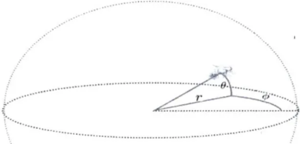
2-7 A shrimp located in 3D space. . ... 21

2-8 Signal representation of the shrimp in ID vector form ... 21

3-1 Illustration of an affine set [5]... . 25

3-2 Examples of convex sets; the line segment between any two points is contained in the set. ... . 26

4-1 v1, v2, v3 are vectors in the dictionary, and y is the function that we would like to decompose. ... 31

5-1 The original signal is in blue, the red is a possible signal constructed from sampled points shown . ... 34

5-2 The measurement captures the spread of the sparse signal, transformed by the basis vectors . ... 36

6-1 Performance of CVX in presence of noise. ... 43

6-3 6-4 6-5 6-6 6-7 6-8 6-9 6-10 6-11 6-12 6-13

6-14 TwIST performace at OdB SNR, varing sparisty levels and t Performance of TwIST in presence of noise. . . . .

OMP reconstruction given exact number of shrimps. OMP reconstruction given 10x number of shrimps. Illustration of 2% sparsity in 2D space. . . . . Illustration of 18% sparsity in 2D space. . . . . CVX performance at different levels of sparsity... OMP performance at different levels of sparsity... TwIST performance at different levels of sparsity... Performance of CVX with respect to sparsity and noise. Performance of OMP with respect to sparsity and noise. Performance of TwIST with respect to sparsity and noise.

6-15 Performance of CVX, OMR, TwIST at OdB SNR, varying sparsity (TwIST

optimized). ...

6-16 Data provided by ROMANIS. ...

6-17 Reconstruction results on real data from OMP. ... 6-18 Reconstruction results on real data from TwIST. ...

6-19 Reconstruction results on real data from OME, less sparse solution. . 6-20 Reconstruction results on real data from TwIST, less sparse solution.

. . . . 45 . . . . 45 . . . . 45 . .. . . . . 46 . . . . 46 . . . . 47 . . . . 47 . . . . 48 . .. . . . . 49 . . . . 49 . . . . 50 au. . . . . 51 52 53 54 54 55 55

Chapter 1

Introduction

There are many technologies that rely on underwater acoustics, such as sonar systems. The surrounding environment often plays an important role in these applications in real life. Noises from the surroundings can sometimes hinder the effectiveness of these applications, while at other times these noises can be exploited, for example as sources of illumination [10]. Understanding the spatial distributions of these acoustic signals can be useful in working to mitigate or amplify their effects.

A common source of these noises are marine animals. The snapping shrimps snap

and release cavities, by which snapping noises are made. They are present in shallow waters. Snapping shrimps makes impulse-like sounds and are sparse in the environment

[10]. The unique shape of their acoustic signal they emit, and their sparsity in the ocean

allows the use for certain mathematical approximation in modeling the system of which the wave propagates and the sensor senses, and certain methods to reconstruct their signals.

The contents of this work focus on implementing such a system that simulates the underwater environment with snapping shrimps and reconstructs the original sig-nals. Three methods of reconstruction -Disciplined Convex Programming, Orthogonal Matching Pursuit, and Compressive Sensing- will be explored, and their robustness to noise, and sparsity will be examined. The methods are tested on real data, and the best method is optimized to achieve best reconstruction results.

1.1

Convex Optimization

Convex optimization finds solutions to optimization problems. Generally, optimization problems are difficult to solve. The solutions either take very long time to compute, or are difficult to find. However, certain types of optimization problems are solvable under acceptable computation time. Convex optimization problems are one of such type. [5]. For a problem to be solved by convex optimization, its objective and constraint func-tions need to be convex. Often times, problems can be transformed such that they have convex objective and constraint functions [5].

Disciplined convex programming (DCP) is a method modeling of convex program-ming, which is a type of non-linear programming that includes least squares, linear programming, and convex quadratic programming. DCP has specific problem setups for users to follow to solve convex programs [11]. CVX is a modeling language devel-oped for modeling convex optimization systems in Matlab. It uses disciplined convex programming in Matlab [12] and is the software used in the work for this thesis in the convex programming part.

1.2 Orthogonal Matching Pursuit

Matching pursuit is an algorithm that decomposes and describes a signal in its most important signature components. The set of components, or atoms, is called the dictio-nary. By representing the signal in a way such that it is sparse with respect to the dic-tionary, matching pursuit is able to represent the original signal as a series of weighted

atoms [14]. For example, a typical sinusoidal signal is sparse in the frequency domain. The dictionary for this signal could be composed of Fourier series. Matching pursuit is developed by Zhang and Mallat [14] to compute adaptive signal representations, especially in adaptive time-frequency transformations.

Orthogonal Matching Pursuit (OMP) is a modified matching pursuit algorithm. OMP updates existing coefficients by applying the projection operator to the residual so that the residual is orthogonal to the selected atoms. This allows a improved convergence

rate of OM, compared to matching pursuit for nonorthogonal dictionaries [16]. Or-thongal matching pursuit was developed to provide full backward orthogonality on the residual at every step, resulting in better convergence than Matching Pursuit.

1.3

Compressive Sensing

Compressive sensing is a technique in signal processing that allows for accurate recon-struction of sparse signals given a limited number of measurements and an underde-termined linear system. Traditionally, to recover a signal, enough samples need to be taken to avoid aliasing and reconstruct with good accuracy However compressive sens-ing shows that this rule does not need to hold if we know that the signal is sparse, and the system is incoherent, which means that the system should be able to spread out the sparse signal in the measurement. When the system is coherent, or fails to spread out the original signal appropriately, this technique fails [8].

1.4 Thesis Outline

Chapter two discusses the problem this thesis addresses, including the problem's phys-ical and mathematphys-ical model. Chapters three, four, and five provide more detailed background on the theory of convex optimization, orthogonal matching pursuit, and compressed sensing, respectively. Chapter six shows the results for these algorithms, and their robustness to noise and sparsity, and their performance on the real data. Chap-ter seven discusses the optimization of parameChap-ters in the applied compressive sensing algoritm. Chapter eight is the conclusion.

Chapter 2

Problem Model and Approach

I

2.1

Background

There are many snapping shrimps living in Singapore's shallow waters. Typical species include the smooth snapping shrimp, ornamented snapping shrimp, and many-band snapping shrimp [21]. Their body length is 4-6cm [1], and their snapper claw can be as long as 2.8 cm [20]. Figure 2-1 shows the smooth snapping shrimp, and Figure 2-2 shows the the snapping claw pieces. When the claw of the shrimp snaps, a cavitation bubble is created from the action, and the collapse of the bubble makes an impulse-like sound.

Figure 2-1: The Smooth Snapping Shrimp [21]. 2 cm Figure 2-2: Diagram snapping mechanism A

I'

shrimp and claw

Their impulse-like non-Gaussian noise hinders the performance of linear correla-tors (which work well with Gaussian noise), but can also be used as an illumination

source in ambient noise imaging [17]. The frequency range of the snapping noise is 2-300kHz [10] and the sound pressure of these acoustic sources can be higher than

190dB re 1m 1pPa [2]. Figure 2-3 shows the sound pressure of a snap, measured at 4

cm away, and sequence of the snapping motion taken at 40,500 fps [20].

A 0 75-0 0.50 * 0.25-0 (n 0.00--1.25 -1.00 -0.75 -0.50 -0.25 0.00 025 0.50 Time (ms) B -1.25 ms -1.00 ms -0.75 ms -0.50 ins -0.25 ms 0 Ms +0.25 mns 2& 3 2 cm

Figure 2-3: Sound pressure profile of the snapping shrimp, measured at 4cm away [20].

2.2

Experiment Setup

I

A 2D sensing array is used to capture the surrounding sound pressure. This Ambient

Noise Imaging (ANI) system is called Remotely Operated Mobile Ambient Noise Imaging System (ROMANIS). A photo of it is shown in Figure 2-4. Its sensing array is composed of 508 sensors, populated on a circular plane of 1.3m in diameter. It weighs about half a ton and has a resolution of 1degree at 60kHz [19]. The bandwidth is 25-85kHz, and the weight is 650kg [19].

Figure 2-4: Remotely Operated MobileAmbient Noise Imaging System, developed by Acoustic Research Laboratory (ARL) at the Tropical Marine Science Institute under the National University of Singapore [19].

Each of these sensors measures the sound pressure at a rate of 196 kSa/a [9], which creates a time series data. Not all sensors of ROMANIS were able to provide reading during the measurement - Figure 2-5 shows ROMANIS will all sensors number, and Figure 2-6 shows ROMANIS with numbered sensors that were providing readings.The data is then read, processed by a custom software [19]. ROMANIS is able to produce images of targets at a distance of up to 120m [9].

The measurements taken by ROMANIS are uncaliberated sound pressure and the sound pressures are relative. To convert them to absolute pressure, there is a conver-sion factor is multiplied to the uncaliberated readings. This calibration is provided in Appendix A.

2.3

Mathematical Model

2.3.1

Signal Model

To simulate the system, also known as the 'forward operator' in sparse sensing litera-ture, the signals of the shrimp and the acoustic propagation need to be modeled. As mentioned previously, the snaps made by the shrimps are impulse-like, shown by Figure

Figure 2-5: ROMANIS with all sensors _{Figure 2-6: ROMANIS with all working}

labeled. sensors labeled.

2-3. In this work, the acoustic signals from the shrimp are approximated as impulses.

Our collaborators in Singapore, Professor Mandar Chitre, and Too Yuen Min helped us developed the following formalism and sampling scheme for simulation: A space of azimuth angles, < from -10 degrees into 10 degrees, and elevation angles, 0 from

-10 degrees to 10 degrees are partitioned to 1 degree sections. A range, F of 1 frame

(data point) into 100 frames was partitioned to 1 frame sections. There could be many more frames, but due to the limit in compuation power, it is constrained to 100 in simulation. In other words, a cone-like shaped space is divided into smaller truncated cones, or frustums. This partion scheme is decided based on the angular resolution of the system (1 degree), and the level of similarity between the system propagation vectors.

To reduce the dimension of the signal representation, the three dimensional space partitions are stacked together vertically into a column vector. This column vector iter-ates through the space in the following way: elevation angle, azimuth angle, and range. When a signal is present in one of the frustums, a '1' is present in the corresponding vector location to represent it. Figure 2-7 shows a shrimp in 3D, and Figure 2-8 shows the signal representation of the shrimp in ID vector form.

0 1 2 3 4 5

Figure 2-8: Signal representa-tion of the shrimp in 1D vector Figure 2-7: A shrimp located in 3D space. form.

2.3.2

System Model

The model for the system is formed based on the delay (in frames) in the signal propa-gating to each sensor. The number of frames is found by the following equation:

x x sin(4o)cos(O) + _{y x sin(e) x Fs (2.1)}

C

[15], where r is the time delay in frames, Fs, the sampling rate is 196000Hz), c =

15401 is the speed of sound in water, x is the horizontal distance from each sensor to_S the middle of the phase array, y is the vertical distance from each sensor to the middle of the phase array. The reduction in magnitude of the sound pressure in propagation has not been accounted for in this model for simplification purposes and also partly because the change is small compared to the scale of the problem setup.

This delay is calculated for each sensor to each signal, forming matrix A. This matrix is multiplied by the signal vector to produce the response on the receiver. To make the system more realistic, white Gaussian noise is added to simulate the noise from the electronics.

Here, the mirror image of the sound generated from the reflection at the surface of water has been disregarded. Ideally, the sources emit spherical waves. However, to simplify the model and the calculation, linear approximations are made to the spherical spread of the acoustic waves.

forward operator ill-posed. If the response vectors of two signals are very similar, and substantial noise is present in the system, the algorithms would be less likely to trace back to the true signals, because the characteristics of their responses are masked by noise. When two vectors are close together, their response vectors are similar because the difference in the times their signals reach each of the sensors are very small.

Chapter 3

Convex Optimization

Optimization is used in many real world applications where the best solution is desired out of many that satisfy the requirement. Some applications are portfolio optimization, and data fitting [5]- all of these applications require some kind of optimization with respect to certain constraints, which is similar to our problem which will explained in more detail later in the section. This chapter will discuss convex optimization [5], and the CVX Matlab software.

3.1

Optimization Problems

3.1.1

Problem Characteristics

Optimization problems hold the following form:

minimize fo(x)

(3.1)

subject to fi(x) bi, i = 1, ... m

where x is the vector being minimized,

fo

fi

follow-ing inequality:

f1(ax + P#y) af,(x) + Pfi(y) (3.2)

where x, y E R", and a, c R, satisfying a +

#

There are two main classes of convex optimization problems: least square and linear programming. Least square problems have the following problem setup:

minimizefo(x) = lAx - b = E(ax- _(3.3)

where a' are rows of A. Notice that it does not have a constraint function. The solution is as follows:

(ATA)x =A Tb. _(3.4)

Linear programming problems have the following setup:

minimize cTx

subject to a[ bi,

(3.5)

i=1,..., m

[5]. In correspondence with the scope of this problem and the system mentioned in

Chapter 2, the linear programming model is used for the problem setup.

3.1.2 Problem Setup

The convex optimization problem setup for this work is:

minimize

I|xIJ1

(3.6)

subjectto IIY-AX11 ₂

XIINI

where X is a constant weight factor, N is the noise vector, y is the measurement, and

A is the system matrix. In reference to the linear programming setup, c from 3.5is the

3.2

Theory

To verify the validity of using the linear programming problem setup in convex opti-mization, the functions

lxIII

IIY

3.2.1

Convexity

As Boyd and Vandenberghe explain, an affine set S is one that contains the line through any two distinct points in the set 3.7. That is, S contains the linear combinations of any number of points in it, with the sum of the linear coefficients being 1. For example, the solution set of linear equations S = x : Ax = b is affine. A geometric interpretation is

show in Figure 3-1. x = 0xi + (1 -x 2) (3.7) = 1.2 X1 0 =0.6 X2 0 = -0.2

Figure 3-1: Illustration of an affine set [5].

A convex set S is one that contains line segment between any points in it. Some

examples of convex sets are shown in Figure 3-2

4 Figure 3-2: Examples of convex sets; the line segment between any two points is

con-tained in the set.

All affine sets are convex sets, since they have the line segments constructed from

any two points from it (as defined previously of convex sets).

An affine function is one such that it is a sum of linear functions and constants 3.9, where S is a convex set. For example, ftinctions of the form Ax + b are affine. Affine functions preserve convexity [5].

f S =f (x)|x ES (3.9)

A function

f

f

f (Ox +(1 -)y) Of(x) + (1 - O)f(y). (3.10)

[5]

Here, the convexity of the setup of the problem is shown:

The norm function is convex, for norms greater than or equal to 1, that is:

if u,vCR" and pE[1,oo)

then Iju+vK !l ulK j+jHvjl,

(3.11)

for all u and v.

are convex. By the convexity requirement,

IIOu+ (1 -)vI" = EIOuj

+

O)v;I

K; E |uilp + (1- O)IviIP (3.12)

= 1OIIPul +(1 -O)IIvIIP

It is apparent that y -Ax is convex, because it is affine. More formally,

y -A(0x 1 + (1- )x2) = O(y -Ax 1) + (1 -

O)(y

)-3.3

CVX

CVX is a Matlab package that models and solves disciplined convex programs. In par-ticular, it supports linear programming problems, and functions like l norms, which are used in the problem setup [13]. As mentioned in Chapter 1, disciplined convex programming is a method of formulating problem setup according to a set of rules pro-posed by Grant, Boyd, and Ye [11]. CVX contains many solvers, and the results for this work were produced by the SDPT3 solver.

Chapter 4

Matching Pursuit

Matching pursuit is an algorithm that allows for adaptive signal representation. It de-composes a signal into its most important signature components, also called atoms. The set of atoms form a redundant dictionary [14].

In Chapter 1, it was mentioned that a typical sinusoidal signal is sparse in the fre-quency domain and its dictionary could be composed of Fourier series. However, it does poorly for a signal that is localized in time, because the coefficients would be spread out among the whole basis. One may suggest that it's possible to just represent the signal in the time basis, however, if the signal is a combination of one that is concentrated in time and another that is concentrated in frequency, it would be difficult to represent this combination sparsely. Matching pursuit provides a way for flexible decomposition for any signal, that results in only using a few atoms to represent the most important structures in the signal. Atoms are waveforms that adapt to the structures of the sig-nal [14]. In this case, these atoms have features that adapt to the unique nature of the signal. In this work, the atoms that make up the dictionary are the unique propagation vectors of the signals each possible location.

4.1

Theory

Given a complete dictionary in which the signal is sparse, matching pursuit expands the signal over a small subset of waveforms that belongs to the dictionary. Let 9 be the

dictionary, and 9 that is g. is a vector in the dictionary, and

f

f

f

f =< f, go > g.o + Rf (4.1)

where Rf is the residual after projecting f onto gO. Since go and Rf are orthogonal,

|if 2 - I <f, 12+|> +lIRf 112. (4.2)

In order to express

f

f

I

f,

f

projected on to the set of vectors in the dictionary, excluding the one that has already been picked out and a new residual is formed. This is repeated until a stop criterion is reached [14]. To better illustrate this point, each subsequent residual can be found by

(4.3)

And f can be represented by a sum of the m vectors that's picked out:

f

This decomposition is nonlinear, but it conserves energy, and is guaranteed to con-verge [14].

v1 v2

v3

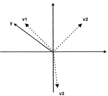
Figure 4-1: v1, v2, v3 are vectors in the dictionary, and y is the function that we would like to decompose.

Figure 4-1 shows y, and the atoms v1, v2, v3. Here, v1 would be chosen first, be-cause the dot product between v1 and y is the largest of all dot products with vectors in the dictionary.

4.2 Orthogonal Matching Pursuit

Orthogonal Matching Pursuit (OMP) is a modified matching pursuit algorithm. Regular matching pursuit has a dictionary that consists of vectors that are not mutually orthog-onal. Therefore, when residuals are subtracted, it can result in introducing components that are not orthogonal to the previous projected vectors. Orthogonal matching pur-suit is different from matching purpur-suit in that the residual is always orthogonal to the chosen set of basis.

OMP updates existing coefficients by applying the projection operator to the resid-ual so that the residresid-ual is orthogonal to the selected atoms. This allows a improved convergence rate of OMP, compared to matching pursuit for nonorthogonal dictionar-ies [18], which is why OMP is usually preferred over matching pursuit, and is used in

this work.

OMP computes the projection operator P as follows:

P = 4((D*4)-1)*

, where 4) is the set of already chosen atoms, and updates the residual by

R" )f = (I - P)R"f (4.6)

[18]. Similar to matching pursuit, OMP conserves energy, which is important for its

convergence.

In [16], the orthongonality is achieved by projecting the residual to the set of chosen atoms in order again, and reevaluate the dot products each time.

4.2.1

Problem Setup

OMP is implemented to solve the follwing system:

y =Ax +N,

with the prior that x is sparse, and N is noise. The inputs to this algorithm are y,A, and k. k is the estimation for sparsity, and tells the algorithm how many signals to try to find, it is not present in this general setup of the problem.

Chapter 5

Compressive Sensing

Compressive sensing is a technique that allows for solving underdetermined linear sys-tems given some priors, with fewer measurements than the typical requirement for signal sampling. It provides accurate estimations for solutions and is used widely as a signal processing technique.

5.1 Theory

5.1.1 Nyquist-Shannon Sampling Criteria

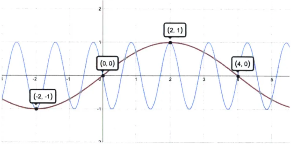
Traditional sampling methods require a sampling rate of at least twice the highest signal frequency for accurate signal reconstruction. Sampling at a rate lower than the Nyquist-Shannon sampling theorem could result in aliasing. Take the following example in Figure 5-1 the original signal is in blue, if we sample this signal using the points shown, the red signal could be constructed, which is incorrect.

2

(0,0) (,0

Figure 5-1: The original signal is in blue, the red is a possible signal constructed from sampled points shown.

Compressive sensing states that the Nyquist criteria can be violated, as long as cer-tain conditions such as signal sparsity and incoherence (to be defined more precisely later) can be used to compensate for the limited measurements and, thus, still recover the signal accurately

5.1.2 Sparsity and Measurement Requirement

One prior of compressive sensing is that the signal needs to be sparse. A signal is sparse when there are many zeros in its coefficients. In other words, a sparse signal

f,

f = E 1xi~i', (5.1)

where x, are coefficients of <

f,

In some applications, such as images, there may be many nonzero coefficients in the sparse basis, but it would be alright to discard some of the smaller coefficients, and still obtain a good representation of the original. Image compression methods such as lossy

JPEG compression exploit this feature for effective storage of images.

good signal reconstruction. Candes [6] has formulated the relationship between the number of measurements required and the sparsity of the signal to correctly reconstruct:

m > CM2_Slog(n),

(5.2)

where m is the number of measurements, C is a constant, p is the maximum of the coherence between the signal and the field of detection, S is the number of nonzeros in the signal, and n is the total length of the signal [8].

5.1.3

Incoherence

Having a sparse signal is not enough for compressive sensing to work. Another impor-tant factor that the system needs to satisfy is that the signal needs to be non-sparse in the measurement domain. In particular, there needs to be incoherence in mapping the signal to the measurement. This system needs to be able to spread out each sig-nal, so that even with very few measurements, the characteristics of the original is still captured.

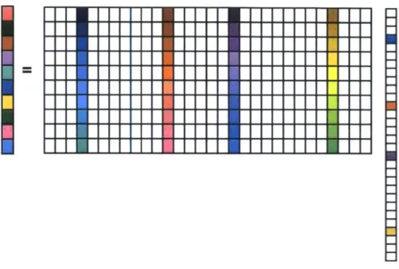
Figure 5-2 demonstrates this concept. The left colored column represents a vector that is the linear combination of the products of sparse coefficients (represented by the colors on the right) and their basis vectors. The colored columns in the matrix shows the atoms that the sparse entries picked out. The left column, the measurement, has the spread of each sparse entry. The shape of the matrix (having more columns than rows) confirms that this is an undertermined system, or an undersampling process, which cannot be solved by typical matrix inversions.

Figure 5-2: The measurement captures the spread of the sparse signal, transformed by the basis vectors.

Coherence can be computed as follows:

tt(<, P) = 0ismax:k,) flI <

4k, 'P

where <D is the sensing basis and 'I is the representation basis [8]. It measures the

correlation between 'I and <D. One can imagine that certain systems will not satisfy

the incoherence requirement. For example, a one to one mapping system will result in large coherence between the sensing and sparse fields. Certainly if we were to wish to reconstruct the sparse signal accurately, all measurements would be needed in or-der to capture the original signal, since the measurement field is sparse itself as well. In addition to the incoherence of the sensing matrix, the Restricted Isometry Property (RIP) is useful to the robustness of compressed sensing, allows for accurate reconstruc-tion under the presence of noise. To understand RIP better, let's look at the following equation

(1 - 5s) xI12 < I XI1 2 (1+ 3s)IIxII12, (5.4)

equation holds for all x that is sparse. When 5s is not too close to one, A is said to obey the RIP order S, and preserves the Euclidean length of the S-sparse signals, hence the nullspace of A does not contain S-sparse vectors [8]. This is important because it ensures that we can recontruct some of these vectors.

5.1.4

Recovery

Compressed sensing recovers via the following convex optimization:

min|xI1 subject tollAx -Y112 e, (5.5)

where ebounds the energy of the noise.

5.2

TwIST

Two-Step Iterative Shrinkage Thresholding (TwIST) is an algorithm developed by Bioucas-Dias and Figueiredo [4] that provides solutions to inverse linear problems. It solves many image restoration and compressed sensing problems. Its approach is to solve the minimization problem:

1

f

2

where y,A, x are the same as defined in the previous sections, A is a weight vector, 4) is a regularization function, and j is an energy matching coefficient. Minimizing this objec-tive function allows for a balance in the solution between the closeness of x to solving

y = Ax, and some optimization factor, which could be some normalization function.

This balance is needed because often in real world applications, there are noises cap-tured in the measurement, therefore an exact solution to y = Ax will not be accurate.

Minimizing the energy or magnitude at the same time ensures that overall the signal is low energy or sparse. The weighing factor A controls how much we would like to min-imized one factor over the other. As mentioned, some typical regularization functions

are 11, 12 norms, or total variation, which is used widely in image reconstruction.

TwIST was developed on the foundations of iterative reweighted shrinkage (IRS) and iterative shrinkage/thresholding (IST) algorithms.

IST algorithms updates the solution by:

xt+1 = (1 - I)x, + I'(xt + K T(y-Kxt)) (5.7)

, where P > 0, and TA is the Moreau proximal mapping defined as

TA(y) = argmin x l 2 .x+ 2II (x).

2 (5.8)

IRS iterates based on the follow equation:

xt+1 = solutionAtx = b (5.9)

, where b = KTy andAt = ADt +K TK, and Dt is a diagonal matrix that depends on x,

and <D

TwIST combines IST and IRS: initialize the solution as xO,

x1 = Fx(xO)

F(x,) = 4'A(x +AT(y -Ax))

(5.10)

(5.11)

and find each iteration thereafter as

xt+1 = (1 - a)xt_1 + (a - P)x +

#f

,where a, 0,

p0

5.2.1 Problem Setup

The parameters of the acoustic localization problem complies with the incoherence and sparsity requirements.

The minimization function implemented in this work is: 1

f

2

Compressed sensing finds the sparsest solutions to the problem. For a multi-dimensional sensing matrix and measurement, compressed sensing strives for the solution that gives the smallest dimensionality. In other words, given a solution that falls onto a hyper-plane, compressed sensing will favor the one that lies on the axis, minimizing the 10 norm. Therefore intuitively, we would like to set the regularization function <D to be

SIlxI

lIxIII

practice, solving minimization of 10 norm is NP-hard. This can be seen from the fol-lowing logic: to find the solution for a 1-sparse signal that is N dimensioned, we need to examine all the values, which results in

(i)

is m-sparse, there are

(')

(N),

hard.

The alternative solution is to minimize the 11 norm, which minimizes the magnitude of the solution, and is covex (also shown in Chapter 3 under Convexity) and much easier to solve. Theoretical results have shown that under sufficient conditions, the optimal solution to 1, norm minimization is also optimal to 10 norm minimization [7].

Chapter 6

Results

In this chapter, results on simulations and real data are shown. First, the system and signal described in Chapter 2 are implemented in simulation. This was done to examine the feasibility of the three algorithms: CVX, OMIP and TwIST, in reconstructing the signals. CVX, OMIP and TwIST are compared in their robustness to noise, sparsity, and a combination of both. These comparisons were made because we would like to know how real-world factors such as the amount of noise in the measurement, and the number of shrimps in the space affect the accuracy these methods. Then, the three algorithms were implemented on the real data from ROMANIS.

6.1 Simulation

Simulations are made based on the system explained in Chapter 2. The following sec-tions show the results of the three algorithms's robustness to noise, sparsity, and their

combination.

6.1.1

Robustness to Noise

There are many sources of noise in the experiment. Noise in this our case is any un-wanted signal. For example, there is noise resulting from signals emitted by sources

noise from the electronics of the experimental system. Since noise is a component that needs to be taken into account in the real world system, we would like to find out how different levels of noise affect the signal reconstruction accuracy of the algorithms.

Noise is usually quantified by signal-to-noise ratio (SNR). SNR is usually expressed in the log decibel scale, since signals can have a large dynamic range. SNR is given by:

P

SNR = 101og1o( signal), (6.1)

noise

where P is the power. A SNR of 0 would indicate that the power of signal is equal to the power of noise.

Figures 6-1,6-2,and 6-3 show how each method performs at different noise levels. There were 3 shrimps (signals) in each trial. The performance is evaluated upon the accuracy in the reconstruction of the locations of the signals. The blue line indicates the number of correct locations of signal in reconstruction (true positives), and the red line indicates the number of incorrect locations (false positives) the reconstruction output.

A quick look at the results shows that the algorithms are performing well even at

negative SNR, when the power of the noise is greater than the power of signal. This can seem misleading, but can be explained by the nature of the signal. The signal is very sparse, and hence the power is low, whereas the noise is non-sparse, and the power across the domain can be greater. Therefore, a second axis showing the peak-signal-to-noise ratio is also shown on the plots. PSNR takes into account of the peak value of the signal. PSNR can be calculated by:

1 0g(Peakvalue

PSNR = 10logMo (6.2)

MS E

where MSE is the mean squared error. All three methods have made many errors at low PSNR values.

The results show that the three algorithms fail at around -20dB SNR, or around

5dB PSNR. The results for CVX fluctuates a lot, which is due to the limited number

of trials conducted at low SNR. CVX took many iterations to converge at low SNR, and given the limited computation power, only a few trials were conducted (more trials were

_AMMEF

0'

-4

CVX results: SNR,PSNR

avg number of correct reconstructed signals

avg number of incorrect reconstructed signals

5 -43 -41 -39 -37 -35 -33 -31 -29 --27 -25 -23 -21 -19 -17 -1 SNR(dB) I I I I I --13.7 -10.7 -7.7 -4.7 -1.7 PSNR(dB) I I 7 1 1.3 4.3 7.3 10.3

Figure 6-1: Performance of CVX in presence of noise.

conducted at higher SNR). However, from the plot, we can determine at what SNR CVX starts to fail. One thing to point out about CVX problem setup is that an estimate of noise level is given, and this is not done for OMP or TwIST problem setups. In the next section, the effect of the knowledge of noise in CVX setups is shown when dealing with real data.

OMP plot shows seemingly symmetric curves. This feature is resulted from the al-gorithm setup - OMP requires an input of the number of signals the user is trying to find. And in these trials, the exact number of signals were fed into the system (this also explains the small error bars when SNR is high and when it's low). This might not seem like an appropriate solution when applied to real world data when the number of signals is unknown, Figures 6-4 and 6-5 demonstrates that this is not a concern. Figure 6-4 shows the results for reconstruction given the correct number of signals (3), Figure

6-5 shows the results for the same measurement, given tenfold the correct number of

signals (30). It is obvious that Figure 6-5 has three significant signals, and many very

-U- U 6 E 5 0 4 E 3 2 I f -19.7 -16.7 5 P - __ - -- - - - - - - Mmmqml

I

- ME-n -4MM~_ MMr

OMP results: SNR,PSNR 5

-avg number of correct reconstructed signals

avg number of incorrect reconstructed signals 4-U) E 3 0 E 0 ---39 -37 -35 -33 -31 -29 -27 -25 -23 -21 -19 -17 -15 SNR(dB) -13.7 -11.7 -9.7 -7.7 -5.7 -3.7 -1.7 0.3 2.3 4.3 6.3 8.3 10.3 PSNR(dB)

Figure 6-2: Performance of OMP in presence of noise.

small ones. These three signals are the correct ones. The smaller signals are the extra-neous ones that the algorithm was trying to find because we forced it to find this many signals. The extraneous signals can be easily prevented when processing real data by setting a threshold factor.

The results from TwIST shows a great increase in the number of false positives right after -20dB SNR. It fails very quickly, with growing error at lower SNR. From these three results, OMP fails slower than TwIST and CVX.

TwIST results: SNR,PSNR

avg number of correct reconstructed signals avg number of incorrect reconstructed signals

3 Shrimps in original signal

-22.5 -22 -21.5 -21 I - -_I I I - -. L _____ I __A -20.5 -20 -19.5 -19 -18.5 -18 -17.5 -17 -16.5 -16 -15.5 -15 SNR(dB) I I I I I I I I I I I I I I 2.2 2.7 3.2 3.7 4.2 4.7 5.2 5.7 6.2 6.7 7.2 7.7 8.2 8.7 9.2 9.7 10.2 PSNR(dB)

Figure 6-3: Performance of TwIST in presence of noise.

1

Figure 6-4: OMP reconstruction given ex-act number of shrimps.

Figure 6-5: OMP reconstruction given 10x number of shrimps. 45 30 28 26 24 22 20 18 16 14 12 10 8 6 4 2 Cn 0. E -c 0 -o E :3 -23 I I I

-2-6.1.2

Robustness to Sparsity

In addition to how the methods perform under noise, we would also like to explore how they perform at different levels of sparsity. Research on directionality of acoustic signals from shrimps has shown that the signals are roughly isotropic, or uniform in all directions [17]. Therefore in this set of simulations, different number of shrimps are placed randomly in space in a unform distribution. The three algorithms are then tested in their robustness to sparsity, and no noise is added. TwIST and OMP specifically have sparsity requirements - both work under the assumption that the original signal is sparse.

Figures 6-6, and 6-7 give a sense of how sparse the space would look like with 1000 shrimps present (2% non-sparse) and 8000 shrimps present (18% non-sparse). Figures

6-8, 6-9, and 6-10 show the robustness of the methods with respect to signal sparsity.

Same as previous results, the y-axis is the number of shrimps, the green line is the ground truth of the number of shrimps in original signal, the blue line is the number of correct recontructed locations (true positives), the red line number of incorrect re-constructed locations (false positives), the black line (only apparent for TwIST results) is the total number of reconstructed signals (sum of true positives and false positives). The sparsity ranges from 2% to 18%.

400

3 J5

100 200 300 400 500 600 700 800 900 1000 100 200 300 400 500 600 700 800 900 1000

Figure 6-6: Illustration of 2% sparsity in Figure 6-7: Illustration of 18% sparsity in

CVX results: sparsity

avg number of correct reconstructed shrimps avg number of incorrect reconstructed shrimps

0 2000 4000 6000 8000 10000

number of shrimps in signal

Figure 6-8: CVX performance at different levels of sparsity.

OMP results: sparsity

0 2000 4000 6000 8000 10000

number of shrimps in signal

Figure 6-9: OMP performance at different levels of sparsity.

I

I1

%-E

E

avg number of correct reconstructed shrimps avg number of incorrect reconstructed shrimps

10000 8000- 6000- 4000-2000 -00 -2000

TwIST result: sparsity

10000 1___I

avg number of correct reconstructed shrimps

9000-. _{avg number of incorrect reconstructed shrimps}

total signals reconstructed 16 8000-) 7000-0 6000- 5000-E 4000-U, 3000-(D E 2000- 1000-0 -2000 0 2000 4000 6000 8000 10000

number of shrimps in signal

Figure 6-10: TwIST performance at different levels of sparsity.

The results show that CVX has correctly reconstructed all signals regardless of spar-sity, while OMP and TwIST reconstruct with some error at low sparsity. OMP recon-structs well up to 7% (3000 shrimps), at which point it starts to fail rather quickly. TwIST performs slightly worst than OMP at 7% and lower, but does a better job at lower sparsity. The total number of reconstructions that TwIST also retrieves is close to the ground truth, without knowing the exact number as compared to OMP

6.1.3 Robustness to Noise and Sparsity Combination

The previous two subsections show the ideal cases when each factor noise or sparsity is isolated. In reality, both of these factors would be present. Therefore, we would like to see how the methods perform under the presence of both, shown in Figures 6-11, 6-12, and 6-13. Here the x-axis is the sparsity level, and noise levels are represented by lines of different colors. The y-axis here is the percentage of correctness in reconstruction.

0-0 : 0, 0 4-0 0 0L 1 0.8. 0.6 -0

CVX result: sparsity and snr

.4

F

0.2

F

0

0 1000 2000 3000 4000

number of shrimps in signal

5000

Figure 6-11: Performance of CVX with respect to sparsity and noise.

OMP result: sparsity and snr

0 1000 2000 3000 4000

number of shrimps in signal

5000

Figure 6-12: Performance of OMP with respect to sparsity and noise.

I

F

-Figure 6-13:

TwIST result: sparsity and snr

snr=0 snr=-5 snr=-10 -snr=-1 5 C_ 0 : 0 0 a 0 0) 0 C) 0) () 0D

a)

number of shrimps in signal

Performance of TwIST with respect to sparsity and noise.

The plots show that at low noise level (high SNR), CVX performs the best with vary sparsity, and at high noise level (low SNR), all methods perform similarly

TwIST, fine-tuning

Before we move on to conclude that CVX is the best out of all algorithms, there is a variable in TwIST that can be optimized but has been fixed in the past. This parameter is A, the weight factor of the regularization function. A is used to vary the importance between the regularization function and the closeness of x to the solution of y = Ax. It makes sense that as the power of noise approach 0, the true x is equal to the solution to y = _{Ax. On the other hand, as the level of noise increases, more weight should be}

placed on the regularization function, to emphasize the sparsity so as to, hopefully, beat the noise. This weight affects both noise and sparsity levels.

In this subsection, we want to see how varying the A changes the performance of TwIST at different sparsity level given a constant amount of noise. In addition, we com-pare the performance of TwIST using the best A with previous results of CVX and OMP

50

I

'1

Since the performance between the 3 methods varied the most at OdB, A is optimized at this noise level.

Figure 6-14 shows how TwIST performs at varous A values. To not just set A to any arbituary value but rather make it dependent on the measuremnt, we compute it by

A = TmaxATy , where r is a constant and we use ATy as an estimate for the initial solution 1. I

.o

wIST

result: sparsity and snr=O at various

T

1000 2000 3000 4000

number of shrimps in signal

5000

Figure 6-14: TwIST performace at OdB SNR, varing sparisty levels and tau.

The plot shows that a u value of 0.05 works well at low sparsity levels. This value is chosen because we do expect that there is sparsity in the shrimp population in the ocean. Figure 6-15 shows a comparison of all three algorithms, with TwIST optimized. It is apparent that TWIST outperforms CVX and OMP Other optimization parameters can be set for OMR, such as the limit on the residual, however, it would affect how well OMP performs under noisy and non-sparse conditions.

t=0.002 t=0.005 t=0.01 t=0.05 t=0.01

'This estimation was developed by Yi Liu

C:

sparsity and snr=O, CVX vs TwIST vx OMP

o

0.3-(D

number of shrimps in signal

Figure 6-15: Performance of CVX, OM, TwIST at OdB SNR, varying sparsity (TwIST optimized).

6.2

Real Data

After examining the methods in simulation and understanding their robustness to noise and sparsity, the three methods were then applied to the real data acquired by

ROMA-NIS. Figure 6-16 shows some real time data. The x-axis is the time in frames, and the

y-axis is uncalibrated pressure. A section of this data was taken for evaluation using the three algorithms, it is denoted by the box in the graph.

10

time series of data

Figure 6-16: Data provided by ROMANIS.

6.2.1 Recontruction on Real Data

For reconstruction, it is assumed that the shrimps are stationary in the short moment, and they are emitting signal at the same instance. CVX was not able to converge on this data. It is possible that part of this non-convergence is due to its requirement on the input of noise. Although different amounts of noise were given as input to try out (they were computed as a function of signal power, at 0.01 times signal power all the way to 100 times), CVX did not converge. This inability to converge has to do with the fact that the noise is unknown. In simulation, CVX was able to converge when the estimated noise level is close to the true noise level. Therefore, even though different levels of noise were tried as inputs, CVX could not converge unless it's very close to true noise, which is unknown.

However, OMP and Twist were able to converge, and produced similar results, shown in Figures 6-16 and 6-18. There are small discrepancies in the magnitude of each signal in the reconstruction, however, the signal locations matched up exactly be-tween the results from OMP and TwIST. Even though we do not have ground truth

-it is very difficult to know which shrimp made which signals in the vast ocean, this consistency across two methods is very promising.

OMP result

Position

Figure 6-17: Reconstruction results on real data from OMP

TwIST result 0 0-0 -0 0.5 1 1.5 2 2.5 Position

Figure 6-18: Reconstruction results on

3 3.5 4 4.5

x 104

real data from TwIST.

Since the number of shrimps present is unknown, less sparse solutions are also pro-duced. Figures 6-19 and 6-20 show less sparse results obtained by OMP and TWIST. Once again, the results line up, showing promising consistency.

54

I

(D 3 cz 2-> 15000 10000 5000 0

OMP result

-it~

IITT

Position

Figure 6-19: Reconstruction results on real data from OME less sparse solution.

TwIST result 2000 0000- T 8000- 6000- 4000-2000 -1-0 0.5 1 1.5 2 2.5 Position 3 3.5 4 4.5 x 104

Figure 6-20: Reconstruction results on real data from TwIST, less sparse solution.

55

I

Chapter

7

Conclusion and Future Work

7.1

Conclusion

Snapping shrimps living in shallow waters make impulse-like acoustic signals. These signals are a source of noise for underwater acoustic technologis. Since the signals are

highly non-Gaussian, they are difficult to remove by linear correlators. At the same time,

the signals emitted by the snapping shrimps show isotropic properties, which supports the idea that the signals can be appropriate sources for ambient noise illumination.

This work has developed a theoretical approximation for the snapping signals, and the sensing system which encapusulates the propagation as well. The formulation of this research problem has deem it an undertermined problem. Three common ap-proaches to solving this type of problem are introduced, and an algorithm from each has been picked out for implementation. The algorithms are: CVX, OMR, and TwIST.

The three methods were first implemented in simulation and tested on their robust-ness to noise, and sparsity. They were then tested on real data set, in which OMP and TwIST showed promising consistency in their results, while CVX was unable to con-verge. Since there is no available information on ground truth, the consistency is best

7.2

Future Work

There is still space for future work on this topic. The system model can be made to be more accurate - for example, it can take into account of the spreading losses due to the expansion of the spherical source wave, and transmission losses due to the absorption and viscosity of the sea water. A good first order approximation of the attenuation loss is the spherical spreading. In addition, a better system can be created by expanding the ranges of coordinates - have

4),

signals, and this is another area to look into for future improvements.

The model can be extended to another dimension: time. Setting up a system matrix that takes into account of the time difference between the snaps of shrimps is more accurate to real life situations. Although at the same time, this requires much more computational power, and should probably be done with parallel computing.