Aggregation for Modular Robots in the Pivoting Cube
Model
M od elMASSA
H M f SNTITUTEby
OFTECHNOLOGY-.Sebastian Claici
SEP 28
2016
B.S., University of Southampton (2014)
LIBRARIES
Submitted to the Department of Electrical Engineering and
Computer Science
in partial fulfillment of the requirements for the degree of
Master of Science in Electrical Engineering and Computer Science
at the
MASSACHUSETTS INSTITUTE OF TECHNOLOGY
September 2016
Massachusetts Institute of Technology 2016. All rights reserved.
Author. .
Signature redacted
Department of Electrical Engineering and Computer Science
August 30, 2016
Certified by ...
Signature redacted
Daniela Rus
Professor of Electrical Engineering and Computer Science
Thesis Supervisor
Accepted by ...
Signature redacted .ejs...
/
K-
UJ
Leslie A. Kolodziejski
MITLibraries
77 Massachusetts Avenue Cambridge, MA 02139 http://Iibraries.mit.edu/ask
DISCLAIMER NOTICE
Due to the condition of the original material, there are unavoidable
flaws in this reproduction. We have made every effort possible to
provide you with the best copy available.
Thank you.
The images contained in this document are of the
,best quality available.
Aggregation for Modular Robots in the Pivoting Cube Model
by
Sebastian Claici
Submitted to the Department of Electrical Engineering and Computer Science on August 30, 2016, in partial fulfillment of the
requirements for the degree of
Master of Science in Electrical Engineering and Computer Science
Abstract
In this thesis, we present algorithms for self-aggregation and self-reconfiguration of modular robots in the pivoting cube model.
First, we provide generic algorithms for aggregation of robots following inte-grator dynamics in arbitrary dimensional configuration spaces. We describe solu-tions to the problem under different assumpsolu-tions on the capabilities of the robots, and the configuration space in which they travel. We also detail control strategies in cases where the robots are restricted to move on lower dimensional subspaces
of the configuration space (such as being restricted to move on a 2D lattice). Second, we consider the problem of finding a distributed strategy for the ag-gregation of multiple modular robots into one connected structure. Our algorithm is designed for the pivoting cube model, a generalized model of motion for mod-ular robots that has been effectively realized in hardware in the 3D M-Blocks. We use the intensity from a stimulus source as a input to a decentralized control algo-rithm that uses gradient information to drive the robots together. We give provable guarantees on convergence, and discuss experiments carried out in simulation and with a hardware platform of six 3D M-Blocks modules.
Thesis Supervisor: Daniela Rus
Acknowledgments
I gratefully acknowledge the contributions of my advisor, Daniela Rus, and lab-mates in the Distributed Robotics Lab. In particular, John Romanishin has been incredibly helpful in this project, as his mastery of mechanical engineering gave birth to the M-Blocks without which this project would not have existed. I also ap-preciate the thoughtful discussions on reconfiguration shared with Cynthia Sung
Contents
I INTRODUCTION
1.1 Challenges ...
1.2 Our Approach ...
1.2.1 Outline of Technical Approach 1.3 Thesis Contributions ...
1.4 Thesis Outline ...
2 RELATED WORK
2.1 Lattice Modular Robotic Systems ... 2.2 Coverage Control ...
3 BACKGROUND
3.1 Pivoting Cube Model ...
3.2 Aggregation ... 3.3 Reconfiguration ... 3.4 Hardware ...
4 DECENTRALIZED AGGREGATION WITH
4.1 Problem Statement and Assumptions . 4.2 Decentralized Aggregation Control ...
4.3 Stochastic Control ... SENSORY 13 14 15 17 17 18 19 19 21 23 24 24 25 26 29 29 31 34 STIMULI
5 AGGREGATION OF MODULAR ROBOTS IN THE PIVOTING CUBE
MODEL 39 . . . . . . .......-.... -. -. -. -. -. -. -. -. -. -. -. -. -. -. -. -. -. . . . . . . . . . . . . .
5.1 Theoretical Results . . . . 5.1.1 Driving Modules Towards the
Stim ulus . . . .
5.1.2 Driving Modules Together . . . 5.1.3 Stimulus Tracking in R2 . . . . 5.2 Results and Experimental Data . . . . 5.2.1 Simulation Results . . . . 5.2.2 Hardware Results. . . . .
6 CONCLUSIONS
6.1 Lessons Learned ...
6.2 Future W ork ... . .. .. .. ... .. . .. .... . .. .
Maximum Direction of the
39 41 43 45 49 50 52 57 58 58
List of Figures
1-1 Self reconfigurable system: 3D M-Blocks. . . . . . 1-2 3D M-Blocks pivoting moves. . . . .
15 16
Admissible pivoting moves... 24
3D M-Block hardware and electronics. ... 27
Torque vs RPM of flywheel. . . . 28
Aggregation in convex regions. . . . . 31
Control laws for aggregation. . . . . 37
Aggregation with non-convex stimulus. . . . . 38
Pivoting moves. . . . . 40
Coordinates at defining strong and weak admissibility. . . . . 43
Modules moving on fixed scaffolding. . . . ..45
Geometric interpretation of eq. 5.4. . . . . 47
Geometric interpretation of eq. 5.5. . . . . 48
Simulation results. . . . . 50
Simulating aggregation in free space. . . . . 51
Expected number of moves until convergence. . . . . 52
Experimental setup for aggregation algorithm. . . . . 53
5-10 Control in free space using two modules. . . . . 55
3-1 3-2 3-3 4-1 4-2 4-3 5-1. 5-2 5-3 5-4 5-5 5-6 5-7 5-8 5-9
List of Tables
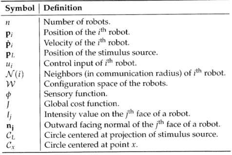
3.1 List of Symbols from Chapters 3-5 . . . 23
Chapter 1
INTRODUCTION
The complexity of biological structures across scales from the molecular to the macroscopic is the result of self-organization processes. Central to these processes
is the aggregation and reconfiguration of matter into a variety of morphologies. Self-assembly confers on biological cells the ability to produce an almost unlim-ited variety of structures [39, 40]. It is no surprise that the flexibility, reliability and speed of self-assembly has attracted interest from an engineering
perspec-tive [41, 43].
One clear advantage self-assembling systems have over purpose built robots is their tolerance of failure. Faulty modules can be swapped out on the fly and replaced by healthy modules. This almost infinite adaptability allows not only for a great number of morphologies, but also ensures the robustness of the system as a whole.
If such modular robots are programmable, can communicate, and are capable of detaching formed connections, they can be exploited to form almost any multi-module configuration. Such abilities would greatly facilitate fabrication techniques such as material printing, would allow for targeted complex anti-viral systems to be deployed seamlessly, and would yield heterogeneous tool sets thus facilitating ease of use. Nature's molecular self-assembly systems do not have the same free-dom, but are able to exploit conformational dynamics to switch between states and can thus achieve hierarchical sequencing of assembly steps. It is a challenge to
reproduce the staggering complexity of natural self-assembly systems in modular robotic systems with only single state modules.
The problem we address in this thesis is aggregation. Aggregation is the pro-cess by which a group of scattered robots gathers in a single location to be able to share information or overcome larger obstacles. The aggregation process can be performed relying on long range communication between robots, but as mod-ular robots are meant to be deployed in remote and unknown scenarios, relying on communication is untenable. Instead, we develop the problem assuming all robots are capable of sensing a environmental stimulus. For example, in planetary exploration applications, the robots may have a light sensor to detect the position of the sun, or a compass to detect changes in the magnetic field. Such sensors are usually small, lightweight, and fault tolerant. The robots may even be endowed
with several redundant sensors to further increase robustness.
In this thesis, we develop the theory of self-assembly by providing algorithms for the aggregation of modular robots under mild conditions. To the best of our knowledge, these algorithms are the first of their kind to be developed for the specific task of aggregation. We build on our previous work that introduced the M-Block [26] and 3D M-Block [25] hardware modules (Fig. 1-1), in addition to theo-retical work describing reconfiguration algorithms in the pivoting cube model [36].
1.1
Challenges
In an attempt to build a self-sufficient modular robotics system there are many challenges that need to be addressed.
From an algorithms perspective, aggregation must be performed in a fully decentralized manner without assumptions about terrain topology, inter-module communication, or reliability. The algorithms must be agnostic to the underlying hardware. As the number of modules in a self-assembly system can grow to the millions, our algorithms must also scale. In particular, we cannot rely on global information to make local decisions as limited communication capabilities make
Figure 1-1: The 3D M-Blocks form a self-reconfigurable system of modules that are capable of individual movement through the use of an inertial actuator, and can bond to neighbors through connectors built from permanent magnets.
this infeasible. Once large scales are reached, defective modules also become an issue. The algorithms must be able to deal with unresponsive modules in a clean way. Furthermore, the algorithms must be both space and compute efficient due to hardware constraints.
Hardware limitations must also be taken into consideration. The limited pro-cessing power and memory storage available on the hardware is a limiting fac-tor when designing algorithms for aggregation and reconfiguration. The modules cannot rely on external tools to function. Each module must have adaptable con-trol to allow them to function in a wide range of environments.
This thesis provides a resolution for the problem of aggregation of the 3D
M-Blocks.
1.2
Our Approach
Our approach improves upon existing hardware and algorithms. We provide the-oretical guarantees for the general problem of aggregating a group of n robots in
R" assuming only integrator dynamics. We prove convergence to a single aggre-gate assuming only knowledge of a single sensory function over the environment. We discuss a related problem of aggregation when the modules can only move along a low dimensional subspace of configuration space. Such problems appear when, for instance, turning the robot to a new orientation is expensive, requiring a significant time or power investment.
We provide provably correct algorithms for modular robot aggregation based on simple sensory information. For the discrete case in which modules are con-strained to move along a lattice, we give a move and time optimal algorithm for the case in which the stimulus is a convex function over the environment. As an example, consider robots capable of sensing light intensity gradients spread in a closed convex environment. The light intensity values define a convex function over the domain, and the end goal is for the robots to converge to a position as close as possible to the light source. For the continuous case, we give a probabilis-tically complete algorithm that performs very well empirically.
We have developed the 3D M-Blocks to test our algorithms on a physical plat-form. The 3D M-Blocks as their name suggests are capable of locomotion across all three axes of a cube. The motion primitive in the 3D M-Blocks consists of a pivot by
r
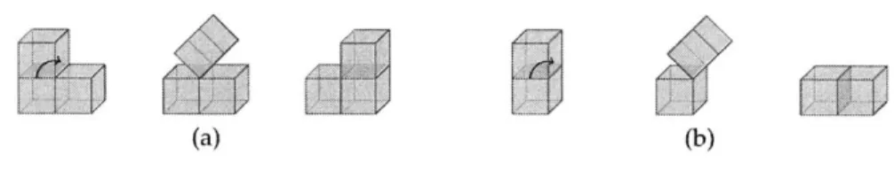
or 7r/2 about an edge shared with a neighboring module or the ground plane (Figure 1-2). While pivoting, a module will sweep out a volume that is greater than the union of the volumes of the starting and final positions.(a) (b)
Figure 1-2: 3D M-Blocks pivoting moves.
We take inspiration from gradient descent algorithms. Our algorithm is a de-centralized optimization with a cost function that tracks a signal in the environ-ment that can be sensed by all robots. Leveraging information on directional signal
1.2.1
Outline of Technical Approach
Our algorithms are based on gradient methods. We assume the existence of a sen-sory stimulus that can be sensed by the robot. Specifically, we assume the robot can determine the gradient of the stimulus function either directly, or by estimating it in a neighborhood around its current position.
We present decentralized provably correct algorithms for aggregation under the following assumptions. First, we assume that the stimulus function is convex, and provide convergence guarantees by reducing to gradient descent. Second, we assume that the robots are capable of communicating with one another, and provide a control law and convergence guarantees by leveraging Lyapunov theory.
We further extend this model to allow for situations in which the robot has a restricted move set, and provide similar convergence guarantees in this case.
We apply these algorithms to the pivoting cube model. Leveraging the more structured environments on which lattice based systems operate, we can improve the convergence rates to linear if we assume the robots are restricted to move on a lattice. Finally, we show how we can efficiently perform aggregation when chang-ing the direction of the robot is expensive.
1.3
Thesis Contributions
This thesis makes the following contributions:
1. A discussion of aggregation for robots following integrator dynamics. We
provide optimal or nearly optimal control laws that drive modules together.
2. A provably correct decentralized algorithm for aggregating modules follow-ing the pivotfollow-ing cube model, where the robot modules can move indepen-dently on a lattice of modules or on the ground. To the best of our knowl-edge, this is the first work that discusses general strategies for aggregation of modular robots.
3. Extensive simulation experiments for aggregation of randomly scattered
mod-ules following global environmental gradients using a decentralized algo-rithm.
4. Experiments demonstrating a hardware implementation of several different distributed aggregation algorithms using the 3D M-Blocks where light is the global external stimulus.
1.4
Thesis Outline
The remainder of this document is organized as follows. In Chapter 2, we sur-vey related work, and discuss limitations with respect to the problem we address. In Chapter 3, we present the pivoting cube model of self-assembly, and provide background on the aggregation problem. We discuss the sister problem of recon-figuration for completeness. Finally, we give a detailed discussion of our current hardware implementation of the 3D M-Blocks hardware, including limitations.
Chapter 4 provides detailed theoretical results for the general aggregation prob-lem in arbitrary dimensional configuration spaces. We give fast convergence guar-antees under different assumptions (e.g. convex stimulus function, or unbounded communication radius), and discuss extensions of the theory to situations where the modules are restricted to move only along a subspace of the configuration space.
Chapter 5 applies the theoretical work of Chapter 4 to the pivoting cube model. We discuss how to overcome the limitations of the pivoting cube model to achieve the same fast convergence rates. In this Chapter, we also provide experimental data (both simulation and hardware) to back our theoretical claims).
Finally, Chapter 6 discusses the lessons we have learned while developing the theory and system, and provides suggestions for avenues of future research.
Chapter 2
RELATED WORK
Modular robotics (or programmable matter) define any system where the individ-ual modules are capable of interacting with one another in non-trivial ways to form increasingly complex systems. Systems that we would describe as modular today have been around for decades. Perhaps the first such system was developed by Penrose in 1957 and 1959 [21, 22].
Primarily, the term modular robotics has come to imply two themes: (1) sys-tems consist of several robots designed to function together, and (2) the syssys-tems address shape formation as the main problem to solve.
Our work builds upon the vast modular robotics literature, from the Penrose tiles, to the ground-breaking work of Fukuda et al [12, 13, 14], to the present day work on various self-reconfigurable models and platforms.
2.1
Lattice Modular Robotic Systems
We situate our work in the context of lattice-based modular robotic systems. Sev-eral models have emerged for self-reconfigurable cubic modular systems [1, 9, 15,
18, 25, 26, 28, 29]. The most prevalent of these is the sliding cube model (SCM)
for which efficient and universal algorithms exist for reconfiguration. The SCM allows modules to slide along their neighbors to achieve motion. In particular, a common feature of the SCM is a nove that slides a cube about two faces of one of
its neighbors to achieve a corner turn. This move proves difficult to implement in practice.
There are however, many attractive theoretical results in the SCM. When strong connectivity (face connectivity) is enforced., there exist
O(12)
algorithms for re-configuring arbitrary 2D shapes [3, 7]. For 3D configurations, algorithms have been developed that achieve reconfiguration if the start and goal configurations do not have topological holes [231. This requirement is imposed as [23] assume that modules that have reached their position in the target configuration will no longer move. If we relax this constraint, we can achieve O(ni) reconfiguration centralized, and O(iP) distributed reconfiguration in 3D shapes [11]. In spite of this attractive body of work, we are not aware of any systems that implement the sliding cube model in 3D. Systems implementing a 2D version of the sliding cube model have been given by [2, 16, 37].Because the sliding cube model is difficult to implement in practice, prompting a move to pivoting cube models of reconfiguration [25, 26]. In the pivoting cube model, modules pivot about one of their edges. Since the volume swept during pivoting is greater than the union of the start and end positions, we must be careful with translating SCM algorithms to this new model.
An 0(ui2) algorithm for reconfiguration was given by [5] assuming edge con-nectivity constraints. In [19], the authors considered pivoting hexagons in 2D and gave a 0(115/2) algorithm for reconfiguration of a restricted set of configurations. An algorithm for reconfiguring pivoting cubes in both 2D and 3D under a strong connectivity assumption was given in [36], however the space of configurations that can be reconfigured is limited.
The pivoting cube model has had successful physical implementations in [26] for modules capable of motion in 2D, and refined in [25] for 3D motion.
While most modular robotic systems have focused on reconfiguration, the 3D M-Blocks are capable of motion in unstructured environments and while unteth-ered. This allows us to talk of aggregation as the problem of localizing and con-necting multiple untethered robots to a single connected aggregate. Recent work
in swarm robotics has demonstrated aggregation and reconfiguration in swarms of up to thousands of robots [27]. However, this work has been restricted to 2D structures, and it is unclear how to develop the model further to allow for 3D motion. An example of aggregation in 3D environments is given in [17], but the modules are not capable of self-locomotion and rely on wheeled robots to perform the aggregation. Approaches to aggregation that do not rely on external systems exist [42], but rely on on-board cameras which are still impractically large to be integrated with most modular robots.
2.2
Coverage Control
A problem that bears significant relevance to our work is that of coverage control.
Briefly, coverage control represents broadly a set of algorithms for optimizing the location of multiple robots to maximize coverage with respect to a function de-fined over the environment. For example, we might wish to communicate through ad-hoc wireless networks, in which case we would want to maximize the signal strength obtained through the network. Such work is situated at the intersection of multi-robot path planning [4, 6] and locational optimization [10, 38].
Distributed coverage control has efficient solutions when the distribution of the stimulus over the environment is assumed to be known a
priori
by all robots [8, 24, 301. This assumption was relaxed first in [31], and improved upon in future work [32, 33].Problems in distributed coverage control share many similarities with aggrega-tion: the algorithms must be distributed, and very frequently the robots have only limited sensing and localization capabilities. We point specifically to [31, 32] as examples of distributed coverage control algorithms that share features with our aggregation algorithms.
The problem we solve is fundamentally different, however. We wish to control the final shape of the robots and their relation to one another. Specifically, we aim to minimize the distance between robots (thus form an aggregate), without
considering the fitness of the robots' position with respect to a sensory function as is the case with coverage control algorithms.
Chapter 3
BACKGROUND
Table 3.1: List of Symbols from Chapters 3-5
Symbol Definition
n Number of robots.
P; Position of the ith robot.
p;
Velocity of the ith robot.PL Position of the stimulus source.
Ili Control input of ith robot.
.'V(i)
Neighbors (in communication radius) of ith robot.W Configuration space of the robots.
Sensory function.
J
Global cost function.i Intensity value on the
jth
face of a robot.nj Outward facing normal of the jth face of a robot.
CL Circle centered at projection of stimulus source.
Cx Circle centered at point x.
We begin by describing the underlying assumptions in this thesis in more de-tail. Specifically, we describe the pivoting cube model: the motion model that our hardware implementation is based on. We describe the problems of aggrega-tion and reconfiguraaggrega-tion to provide intuiaggrega-tion into the theoretical contribuaggrega-tions that follow. Finally, we conclude this chapter with a description of the 3D M-Blocks hardware and its limitations.
(a) (b)
Figure 3-1: Admissible pivoting moves.
3.1
Pivoting Cube Model
As its name suggests, the pivoting cube model comprises cubic modules that are move by pivoting about their edges. In the sliding cube model a move is possible if the start and end positions are adjacent, and the end position is unoccupied.
By contrast, in the pivoting cube model, the volume swept by a module during a
move must also be unoccupied since a cube is longer along a diagonal. This greatly restricts the set of moves allowed.
In our model, a cube pivots the maximum possible before it comes into face contact with another module. Two modules are connected if they share a face.
The pivoting cube model is attractive because it implements a realistic move set that can easily be translated into a hardware implementation. For example, the corner step move shown in Figure 3-1b is a pivot by r radians, while in the sliding cube model, a similar move is unrealistic.
We define the ground plane y = 0 and restrict ourselves to configurations C E R.O
3.2 Aggregation
Aggregation is the task of connecting modules that are initially scattered in an environment into one single connected whole. This task is easy when the modules are capable of relative localization through sensory input (e.g. message passing), but significantly more difficult when such information is not readily available.
In the 3D M-Blocks (see Figure 3-2 and also 3.4), communication is only guar-anteed in point-to-point contact. Therefore, instead of relying on communication,
we formulate the problem as an optimization over a sensory stimulus and use gra-dient ascent strategies to perform aggregation. Each face of a 3D M-Block has an ambient light sensor that outputs a scalar value in a bounded range. These read-ings can be used to obtain a direction of steepest increase and to steer the module
towards the aggregate.
We generalize this setting as follows. Let VV be a bounded two dimensional region, and let IT : -> R be a sensory function that returns the intensity of the
stimulus at each point in
V.
For aggregation of n robots into a single connected component, we require that 0 be convex. Let pi : [0, inf) -+ IT be the position function of each module i for 1<
i < i.We distinguish between two problems:
Lattice Aggregation. The modules are restricted to lie on a lattice embedded in
W. The modules are capable of motion along the x and y axes of the lattice.
Free Space Aggregation. To better model the actual behaviour of the 3D M-Blocks, we endow each module with a direction vector ui (t). Modules can move along the direction vector ui(t), or they can attempt plane changes which reori-ent the module along a differreori-ent direction vector ui'(t) while also adding random noise to its position vector pi'(t) = Pi(t)
+
where ( is drawn from a distribution over IT. For probabilistic completeness, we require that j have non-zero density almost everywhere in W.3.3
Reconfiguration
Once aggregation has been achieved and the modules are in a single connected component, we turn our attention to the problem of reconfiguration.
A configuration C is a set of unit cube modules on a cubic lattice. Let ICI be
the number of modules in configuration ICI. We will identify a module with an index i into this set. We can assign a coordinate system such that each module i is at integer coordinates (xi,
yi'
7).con-figuration graph G = (V, E) with vertices V
{ili
isa module in C} and edgesE
{
(i,j) ji,j are connected in C}. The configuration C is connected if theun-derlying graph G is connected. As a surface in R3, C has a boundary aC, and a complement R3 \ C.
The problem of reconfiguration can be formulated as follows. Given configura-tions C, and Cf where
IC,
I = ICf , find a set of feasible configurations (CS, C1, .. ,CT)such that the following conditions hold:
" Termination: CT = C1.
" Validity: For each t, Ct can be obtained from Ct-1 by pivoting a set of modules
in Ct-1.
" Collision Avoidance: For each set of moves, the volumes swept by the modules
during execution must not overlap.
* Connectivity: For each t, the configuration graph of Ct is connected.
In addition, we can distinguish between solutions by counting the number of moves required to achieve reconfiguration. Formally, a move is any single pivot by a single module. For instance, if several modules are required to move to achieve reconfiguration, we count one move for each. A solution that requires fewer moves overall is better than one that requires more moves. For practical purposes, we would also want to distinguish between moves based on their empirical difficulty. This can be achieved by assigning non-uniform weight to each move and prefer-ring moves with smaller cost.
3.4 Hardware
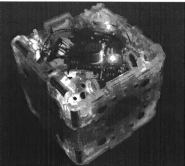
The 3D M-Blocks are modular self-reconfigurable robots which use inertial actu-ation to reconfigure by pivoting about the edges of the modules (Figure 3-2). 3D M-Blocks move by applying a torque generated by an internal flywheel. To reach
Figure 3-2: Photo showing a 3D M-Block with current hardware and electronics.
very high torque impulses, we employ a mechanical braking system that can gen-erate torques in excess of 2.5Nm in a 10ms window (Figure 3-3).
An internal mechanism allows the flywheel to realign to a set of orthogonal axes X, Y, Z. Each face has eight face magnets and four edge magnets. All faces are rotationally symmetric making the 3D M-Blocks symmetric about three orthogonal planes.
While designed to work best on a structured lattice formed of other modules, the internal actuation mechanism allows the modules to move freely both individ-ually and as assemblies.
Each face of the 3D M-Blocks contains a microprocessor that manages an am-bient light sensor, two RGB LEDs and IR communication electronics. One face contains an accelerometer to allow the module to determine its orientation with re-spect to the central actuator. The modules are capable of communication through an infrared light system. Each face can transmit and receive IR messages on a range of up to 200cm.
When transmitting messages between adjacent modules, the IR light will re-fract through the received face and reflect on the interior of the body, messages
3-14000 RPM 2.5 9000 RPM 5000 RPM 2- 1.5-E z 0 . 0-0 -0.5--1I 5 10 15 20 25 30 35 Time (ms)
Figure 3-3: Torque generated by applying the mechanical brake. Plot shows torque (in Nm) against RPM of the flywheel when the brake is applied. Several experi-ment runs (shown in faint colors) are averaged and the mean is displayed in solid colors.
need to be signed with an initial pattern that can only be detected by sampling the ambient light sensor of the adjacent face.
Chapter
4
DECENTRALIZED AGGREGATION
WITH SENSORY STIMULI
In this chapter, we establish theoretical guarantees on convergence under a gen-eral framework. Specifically, we assume our robots have integrator dynamics, and can sense the gradient of a sensory function 0. We show that for convex ( or for unbounded communication radii, aggregation is always achieved, and the conver-gence rates are bounded. We also explore a constrained version of the problem where robots are restricted to move along low dimensional subspaces of the con-figuration space, and provide convergence guarantees for such situations as well.
4.1
Problem Statement and Assumptions
We study the problem of aggregating ii robots in a bounded set. Let V be a closed bounded subset of RN, and let pi denote the position of the ith robot in W.
Assume the ith robot is capable of communication within a ball of radius r;
denoted by S (p;, ri). Define the sensory function W :AW -- R, where 0
(q)
is theIn what follows we assume the robots follow integrator dynamics
pi
= Ili.where iti is the control vector of the ith robot, and pi is the usual velocity vector. This assumption is common in the coverage control literature[8, 24, 31, 32]. We further assume that each robot has knowledge of the gradient of the sensory func-tion Vp at each point q
C
W.Unlike in coverage control, we do not require that each robot be able to compute its Voronoi cell, nor does each robot have to have any knowledge of surrounding robots.
Under this setting, the goal of each robot is to minimize its distance to every other robot:
1
i(p
i)
E
P - pA
(4.1)
jii
where p-_i = (pl,.. I Pi-1' Pi+1, ..- , p,,). The global cost of the system (pI, ... ., p1) can be written
f (P , .- -,11)P, - Pjl12.
(4.2)
i=1 j=1
Equations (4.1) and (4.2) cannot be optimized directly without knowledge of the position of every robot.
Since 2
- is a metric, we can write using the triangle inequality
11p -
p|
11
2 <1(Ilpi
-
q
112-+1p
-
q
21)J z4i i7 i
for any point q E
W.
Finding a control law that drives all robots to the same position q will also minimize equation (4.1) for all robots.We assume that Vcp is Lipschitz, that is, it satisfies
IIVO(x)
- Vq(y))1 < Cflx-y I for some constant C and all x,-y
E
W.
The Lipschitz condition can beunder-stood intuitively as a bound on the rate of change in a small time frame. We require this condition for several reasons. First, from a practical standpoint there will
al-ways be errors in the position estimation and control law of the robot. If were
to vary unboundedly, small errors can compound rapidly. Second, as we shall see soon, there is a strong correlation between aggregation of robots, and the gradient descent algorithm for finding local minima of functions. To guarantee convergence of the gradient descent procedure, we require 0 Lipschitz continuous.
4.2
Decentralized Aggregation Control
We want to derive a control law that will drive the robots together in a reasonable manner. By reasonable we mean here the following:
1. If
q
is strictly convex, the control law will drive the robots to the same posi-tion. While this may seem like a stringent requirement, note that most point source stimuli (e.g. light or sound) satisfy convexity2. If for each robot W/V C B(p, ri ), then the control law will drive the robots to the same position. Effectively, this condition states that the communication
radius of the robot includes the entire configuration space. All robots must be able to communicate with all other robots.
Figure 4-1: Aggregation of information.
robots distributed in a convex region using sensory
This motivates the following control law:
li = -2 7p(pi) (4.3)
where a is a line search parameter.
Control law 4.3 is a gradient descent method and is guaranteed to converge to a local minima if 0 is differentiable, VO is Lipschitz, and a is chosen to satisfy the Wolfe conditions [20]. The intuition here is that we want the robot to move towards a direction that has the largest drop in intensity of
p,
thus moving towards the minimum of 0. If 5 is globally convex, 4.3 converges to the global minimum for each robot. That is to say, we chose q to satisfymin p (x).
We call 0 strongly convex if it is twice differentiable and satisfies V2p >- dl
for some constant d where I is the identity matrix, and V2p is the Hessian
ma-trix
(4 ..
for i,
j
E
{1,...
,nz
}.
If
p
is strongly convex, then control law (4.3)
converges at exponential rate.
However, we also require that the robots are able to aggregate if they can com-municate over the entire environment (the second requirement). Equation (4.3) does not achieve this for functions that are not globally convex.
To motivate the second control law, consider again the cost function (4.2). The derivative of j with respect to pi is given by
-
(ni
- E)p, pThis suggests the following control law to force robots together:
Ui = --pi +
P.
(4.4)
jcm(i)
where V(i) is the set of robots that robot i can directly communicate with; that is, those robots j for which pj
C
S(pi, ri).Note that in the case of VV
C F(pi,
ri), equation (4.4) reduces to1
We recall that a fixed point of a dynamical system is a point where all first derivatives vanish. It is clear that pi = --) ZcgE(i) pj is a fixed point of the system. We also recall that a fixed point is asymptotically stable if, as time goes to infinity, the system approaches the fixed point. Formally, we can write:
Definition 4.2.1. A fixed point x, of a system t = f (x(t)) zwith x(O) = xo is
asymptot-ically stable if it is Lyapinov stable and there exists a 3 such that if j1xo -
Xell <
3 then
limt.c
j|x(t)
- x01|
=
0.
Here we used the definition of Lyapunov stability. We will not repeat it, but note that intuitively Lyapunov stability is a bound on how far away a system can get from the fixed point if it starts within some distance 6 from the fixed point.
We will use Lyapunov functions to verify the asymptotic stability of our control law [34]. We propose the following Lyapunov function:
Vi =
T,|1pi - p;||
(4.5)
i=1 jE/(i)
We need to check the two Lyapunov requirements for asymptotic stability:
" V(x) > 0.
SVi (x) < 0 for some neighborhood around the mean position.
For the second condition, we have
V;(p-) = Vi(pl) -Ili
=
(N~)|-1)i
E P;
-Pi +
P;
j -i'(i) jENr(i) 2
Since vi (x) < 0 for x
#
)1 N Eg(i) Pj. By LaSalle's invariance principle, thesystem is asymptotically stable to the mean position of the neighborhood.
4.3
Stochastic Control
We consider now the problem of finding a control law for robots that have re-stricted dynamics. Consider the following model:
Definition 4.3.1. A robot is said to have partialliy stochastic dynamics
if
at any time it canselect between two actions:
" Move according to the control law (P I|V)
(u
I
V)for some V
C
W with dim V <
dim W. That is to sal, the motion of the robot is restricted to a subset of free space: for exatiple, a robot moving in two dimensions can be restricted to move only along
a straight line.
" Uniformly sample a subset V' C W to move in. Note that since the position of each robot is a continuous function of time, the current position pi must be included in
the subset V'.
This definition is prompted by the M-Blocks, and expanded further in chap-ter 5.
The conditions on V are that it be connected and closed, convex for the control law to make sense, and that
p
restricted to V remain continuous. Moreover, ifv,. .. , v,, torm a basis of V, we require that the partial derivatives a exist for all
i. If el,. . . , e,, are the basis vectors of R"', the last condition is equivalent to the fact that the linear map g is an isomorphism.
We consider again the problem of driving the modules together. We wish to minimize the global cost (4.2) under this new setting. We first note that if
p
is convex over W, then it is convex when restricted over V. Since V is convex, Ax +(1 -- A)y E V for all x, y E V, and convexity of
p
V follows from convexity of f over IN.We will use the notation V' ~
bl(x,
W42) to denote a uniform sampling from IT of subsets that contain the point x. For a concrete example, consider sampling the set of all lines passing through a point x in two dimensions. This can be accomplishedby sampling uniformly a direction vector y and taking the line x + y.
Therefore, we can adapt the control law (4.3) to
-
PVV
)(pi),
if V(0IV)(pi) # 0,
ui = (4.6)
V ~ U (p i, W), otherwise.
The sampling step is only performed after the robot has reached a minimum of
V (P1 V). The procedure is detailed in Algorithm 1.
Algorithm 1 Stochastic control
1: repeat
2: if there is a direction of decrease in the stimulus then
3: set Ui -1V(PV)(pi)
4: else
5: sample new subspace in which to move
6: until good enough solution is reached
Note that Algorithm 1 is not guaranteed to converge. However, under certain assumptions on the sampling procedure, we can provide convergence guarantees of (4.6) to the true global minimum of the function. By convergence, we mean that there exists some time T such that for all t > T, we have ui = 0. Examples include moving only along different coordinate axes (a variant of coordinate descent [20]).
Let us restrict ourselves to the case where V is sampled uniformly over all
m-dimensional hyperplanes where in < n (also called rn-m-dimensional flats). To sam-ple an r-dimensional flat that contains p;, we can samsam-ple in points x1,.. .., xr from
W, and define the flat as intersection between the linear span of
{ pi,
x1,..., I x}and W.
We will prove the following:
Theorem 4.3.1. If V is sampled unifornly over the set of n-dimensional flats, and P is convex over W, then control lazw (4.6) converges.
We will make use of the monotone convergence theorem which we restate here in a simple form (see [35]):
Theorem 4.3.2. (Monotone convergence) If (an) is a monotone sequence of real numbers,
then this sequence has a finite limit if and only if the sequence is bounded.
We are now ready to prove Theorem 4.3.1.
Proof. Let the pl,..., p7 be the sequence of points for which Vp(p)= 0. By the
convexity of 0, we have O(pj) > p(p2) > ... > p(p7). This series is monotone and bounded since p is bounded. Applying the monotone convergence theorem,
we can conclude that control law (4.6) converges. D
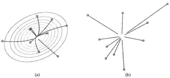
We conclude this chapter with a simulation result. For the simulation, we as-sumed there n = 10 robots placed according to a normal distribution in R2. We use a Gaussian function
as the sensory stimulus with p = 0 and E equal to the identity plus a small off-diagonal term.
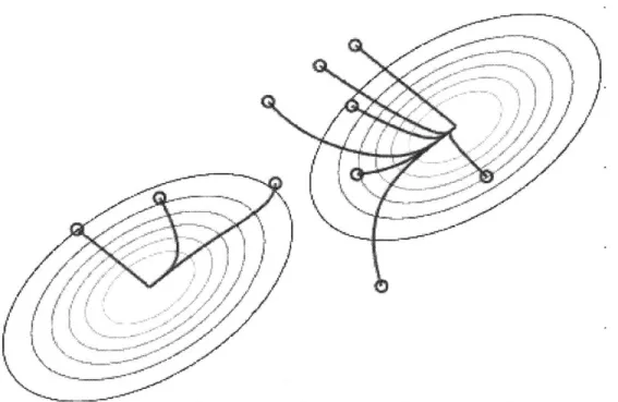
We use control laws (4.3) and (4.4) in two simulation experiments. For control law (4.3), we fix a = 1 as the step size, and perform gradient ascent. Simulation runs are shown in Fig. 4-2. Both control laws converge to a single point, thus achieving aggregation. We note here that convergence rate depends on the choice
/I ...
(a) (b)
Figure 4-2: Simulation of aggregation control laws. (a) Control law (4.3); the robots' initial positions are shown as circles and the trajectories shown as red lines; we draw the contour lines of the sensory function. (b) Control law (4.4); the robots' initial positions are shown as circles with the trajectories shown as red lines.
of parameters and control law. If the robots can communicate with all other robots, then moving towards a shared center can be significantly faster.
Of course, it is always possible that the sensory function has multiple local minima, and after aggregation the robots are split into distant clusters (such an example is shown in Fig. 4-3). However, in such cases it is impossible to achieve a single aggregate without assuming prior knowledge about the structure of the environment, sensory function, or knowledge of the number of robots in the sys-tem. Such assumptions are untenable in our physical implementation using the M-Blocks, and generally untenable for modular robotics systems.
In this chapter, we have looked at the problem of aggregation in a generic fash-ion, assuming integrator dynamics on the robots. In the chapters that follow, we explore a specific example of aggregation in the case of the 3D M-Blocks.
0)
Figure 4-3: A single aggregate is impossible in this scenario. The robots are dis-tributed in an environment with two local maxima and have very limited com-munication capabilities. As can be observed, two aggregates are formed. Without prior knowledge of the number of modules, such scenarios cannot be resolved into a single aggregate.
Chapter
5
AGGREGATION OF MODULAR
ROBOTS IN THE PIVOTING CUBE
MODEL
Following Chapter 4, we implement the algorithms described in the pivoting cube model. The restrictions presented by the pivoting cube model are dealt with new theoretical results. We showcase an example arising from our hardware imple-mentation where the stochastic control described in the previous chapter is impor-tant. We conclude this section with experimental results including simulations and hardware experiments of aggregation.
5.1
Theoretical Results
Let W be a bounded two dimensional region into which we embed a lattice struc-ture C, for example a 2D grid over R2. Assume there are n modules, and let
p1(t),..., pu(t) E N --+ C denote the positions of the modules at time t. All
modules have the same mass and the laws of gravity hold. Each module can pivot about its edges to reach new positions on the lattice. The modules move indepen-dently of one another and require only information about edge connected neigh-bors to determine whether pivot moves are valid. We assume it takes unit time for
(a) (b)
Figure 5-1: Pivoting moves.
a cube to execute a move from one lattice position to another.
Since our focus is on aggregation and not path planning, we assume there are no obstacles in the environment. To achieve aggregation, each module will inde-pendently follow the maximum direction of a stimulus located at position PL. We say that the process has converged if there are no viable moves that would move any module in the environment closer to the stimulus source. We assume the mod-ules are initially scattered throughout the environment, which allows us to restrict our attention to the two-dimensional plane.
The 3D M-Blocks have sensors embedded on each of the six faces that output a number from 0 to 1024 representing the intensity of the sensor readings on that particular face. Let I1,..., 16 be the intensity readings on each of the 6 faces.
If the algorithrm converges at time tj, we try to minimize the maximum distance
between any module and the stimulus source at tf:
minmax
I|pi(tf)
- pMI|.
(5.1)
where PL is the position of the stimulus source and i E {1,. . ., n}.
Since PL is difficult to estimate, each module will attempt to maximize a fitness function that uses the stimulus intensity readings:
1
I:
1(5.2)
{Ijl;
I
O}l 1i O
Equation 5.2 is an average over faces that have non-zero stimulus intensity readings. As we only count non-zero intensities, the maximum is achieved when a module is directly below the source, as then Equation 5.2 reduces to maxi Ii.
5.1.1
Driving Modules Towards the Maximum Direction of the
Stimulus
We will use the notation In to denote the stimulus intensity reading on the face with surface normal ni.
To drive towards a stimulus source, each module must first estimate the direc-tion of the source. This is the purpose of Algorithm 2. This direcdirec-tion is used as a gradient in Algorithm 3 to drive the module towards the stimulus. Algorithm 3 can be interpreted as greedily selecting the move that moves the robot closest to the stimulus source and repeating until convergence.
Any move is a translation that can be written as a sum of at most two face nor-mals (e.g. the move that takes a module from (0, 0,0) to (1, 1, 0) can be written as a sum of (1, 0, 0) and (0, 1, 0)). A move is possible if the volume swept by the module during rotation does not collide with any other module or the environment. We say a move is
weakly
admissible if the intensity reading on at least one of the faces corresponding to the normals is greater than 0. We call a move strongly admissible if the intensity reading on all of the faces corresponding to the normals is greater than 0 (see also Fig. 5-2).We can use this information to provide a estimated direction towards the stim-ulus source. Using the notation described above of nj for the normal of a face, we can estimate the direction of the stimulus source as
jcfaces
Algorithm 2 implements the stimulus direction estimation strategy discussed above.
Algorithm 3 acts as a controller for each module. Note the following: we choose the move whose direction is closest to the direction of the stimulus source esti-mated using Algorithm 2. Also, note that we only iterate over feasible moves in line 4.
Algorithm 2 Estimate direction of stimulus source 1: function ESTIMATESTIMULUSD IRECTION(Cube i)
2: for each face j do
3: I <- STIMULUSINTENSITY(j)
4: ni surface normal to face j
5: return Efaces ,1nn
Algorithm 3 Drive cube towards estimated direction 1: function STEP(Cube i)
2: d - ESTIMATEDSTIMULUSDIRECTION(Cube i)
3: sort moves by distance to d 4: for each move M do
5: let n1,...,nk s.t. ini = M 6: if j
C
1,...,k s.t. hn. > 0 then 7: return M 8: return NIL 9: 10: function DRIVE(Cube i) 11: M +- STEP(Cube i) 12: while M 7 NIL do 13: apply move M 14: M +- STEP(Cube i)We wish to prove the following:
Theorem 5.1.1. For a cube with initial position pi(0) that only performs weakly admis-sible moves there is only a finite set of coordinates at which it can later reside. This set is
the sphere in the 11 norm with radiuis
IPL
- Pi(O)
II
and center PL.
Proof. For our hardware platform, the stimulus is a light intensity reading. In this
case we can use Lambert's law
I.,
O:nj - dj.
(5.3)source read 0. In cases where this does not hold (e.g. sound intensity), we can use just the largest two values and all proofs follow.
As we assume weak adhissibility, the module cannot take a move that would place it farther away in the 11 norm from the stimulus source than pi(O), for such a move would have a component oriented away from the stimulus source, and
would thus not be chosen by Algorithm 3. E
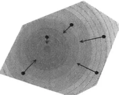
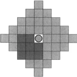
For the 2D case, Figure 5-2 shows the set of coordinates at which the blue cube can reside. In yellow are shown the points satisfying weak admissibility, while in green are shown those satisfying strong admissibility.
Figure 5-2: Coordinates at which the blue module can reside. In green are positions that are stronglyl admissible, while weakly admissible positions are in yellow. The circle represents the projection of the stimulus source onto the plane.
Strong admissibility guarantees convergence as the module can only move closer
to the stimulus source. To ensure convergence with weak admissibility, we require an extra 0(1) memory per cube to detect two step cycles.
5.1.2
Driving Modules Together
We now show that Algorithm 3 converges to the global maximum of Equation 5.2 for one module.
Theorem 5.1.2. Algorithm 3 converges to a single aggregate. Moreover, the
following
two properties will be satisfied:1. There will be a module in the final configuration that is at the closest lattice point to
the projection of the stimulus soirce on the plane. 2. The final configuration has no holes.
To give an example of Property 1, consider several 3D M-Blocks under a light source. Property 1 states that there will always be an M-Block on the lattice point closest to the light source.
Proof. We first prove Property 1. Assume there is no such module. For a module to
be unable to move closer to the stimulus source, there must be other modules one step closer across both directions in the Manhattan norm. This chain of modules is finite and terminates either with a module located closest to the projection of the stimulus source, or with a module that is able to take a move closer to the stimulus source. But we can take this move and repeat the argument. Since the set of possible moves is finite, this process will eventually terminate when there is a module that is located at the closest lattice point to the projection of the stimulus
source.
Assume now that the algorithm converges but there are multiple aggregates. Let CL be the module in Property 1. Find the closest module to CL that is not part of the same aggregate as CL. If this module cannot move closer to the stimulus source, there are modules blocking it, but these modules are then closer to the stimulus source, and thus closer to CL while still part of a different assembly contradicting our assumption that we chose the closest module.
Property 2 follows by an analogous argument to the above.
To determine whether a move is possible only requires local information (knowl-edge of modules connected on each face) about a cube's neighbors in the plane. Each module requires 0(1) time to make a decision about which move to take.
Algorithm 3 thus scales to arbitrarily many modules and converges in time pro-portional to the maximum 11 distance between any module and the projection of the stimulus source on the plane.
5.1.3
Stimulus Tracking in R2
The algorithms developed above guarantee convergence when the modules are restricted to move along a lattice structure. For example, if there is a base of "scaf-fold" modules that are not capable of actuating, but provide support for modules that can actuate, the algorithms above apply. One example is in automatic manu-facture of buildings: a few modules can be active at a time, and reside on a base of inactive modules. Selectively aggregating just a few modules at a time, simple shapes such as cuboids and prisms can be constructed (Fig. 5-3).
j0
Figure 5-3: Modules moving on fixed scaffolding. Green modules above are mo-bile, while the orange modules forming the bottom layer are not capable of motion, but form a lattice on which the former move. In this scenario, algorithms (5.1)(5.2) can be used as the scaffolding acts as a lattice.
However, if there is no lattice base, the M-Blocks develop a very high torque when performing a plane change. The forces generated during this maneuver will cause the M-Block to shake violently and lose its initial orientation. Thus, we can-not rely on the lattice assumption and must develop algorithms to deal with the
We relax our requirement of deterministic convergence and give a probabilisti-cally complete algorithm that at every step with high probability will drive the 3D M-Block closer to the stimulus source.
We assume the M-Block can be modeled as a point x endowed with a direction vector u. The stimulus source is a circle centred at XL with radius RL (write CL for this circle). The M-Block has reached the goal if x XL 2 < R1_. In continuous space, the control strategy is:
1. Move along u or --u to closest position to light source. This effectively
projects XL onto the line passing through x that has direction u.
x' = X + uT(xL - x)u
2. If the goal is not reached, sample uniformly from a circle centred at x' with radius R, (write C, for this circle), and sample a new direction vector u uni-formly at random (equivalent to sampling the slope of the line that passes through the new point).
Intuitively, steps 1 and 2 describe a situation where the module moves as much as possible towards the stimulus source along the line it is currently oriented to-wards, and when it cannot improve its position further, the module performs a reorientation maneuver. Recall from Section 4.3 that this procedure is guaranteed to converge eventually. In what follows, we provide stronger guarantees and em-pirical results for the particular case of the M-Blocks.
We call one complete execution of 1 and 2 (moving along line and sampling new position) a single step. For the very first jump we assume the first step has been performed.
We care about the expected number of steps needed for the M-Block to reach the goal. The probability that the goal can be reached in one step is given by:
|C1
nCCJ|
CL OCC
I
arcsin |Ixs XILI|2Pr[one step] = R2 + (1-
2
fT
'J dS (5.4)-T
/R2 jJdS
7T S Swhere S = C, \ CL.
CA
CL
Figure 5-4: Geometric interpretation of eq. 5.4. Either the new position is in the grey intersection, or averaged over all other positions, the new direction vector is within the blue angles.
The geometric interpretation of eq. 5.4 is that the goal is reached if either the new random position is within CL (the first term in eq. 5.4), or the new direction vector will move the cube into CL. This only happens if the direction vector (or its inverse) is within the two tangents from the new point to the circle.
A new position x' is better than x if
Ix'
- XL 2 clix
- XL I2. Notice that thisis the same as the problem of reaching the goal in one step with RL replaced by
x-XL 112. We are trying to move into the circle centred at XL with radius ||x - X112
(the old distance). Call this circle C1 and its radius R 1. The probability of improving
the position is then given by
Pr [improve] = Pr [one step]
+
(1 - Pr[one step]).IIxS-xIJ-(5 )
C
nC|
|C1 n Cx|
2
arcsin
-
2(5.5)
7-R2
-T2f dS
/-TS S
This is much larger than Pr [one step] as the function is increasing with distance when
XI
C
CL
Figure 5-5: Geometric interpretation of eq. 5.5.
Since the surface integral in both equations is difficult to evaluate, we lower bound the probabilities by assuming all points within the regions being intergrated over are distance
11x - XL112
+
Rx away from the stimulus source.We now establish the following results.
Proposition 5.1.1. Pr[one step] > 0 if the space is convex and bounded.
If we show that Proposition 5.1.1 is true, then we have effectively shown
prob-abilistic convergence of our algorithm, as everywhere on the set, the probability that we will converge to the optimum solution is non-zero.
We now proceed with the proof:
Proof. If CL and C, intersect, then the first term is strictly positive. Otherwise 1x
-XL 112 > R L and the integral term will be strictly positive.
We note here that the algorithm also extends for bounded sets that are not nec-essarily convex in R2 but on which the stimulus function