Aggregating Building Fragments Generated
from Geo-Referenced Imagery into Urban Models
Barbara M. Cutler
Submitted to the Department of Electrical Engineering and Computer Science in Partial Fulfillment of the Requirements for the Degree of
Master of Engineering in Electrical Engineering and Computer Science at the Massachusetts Institute of Technology
19 May 1999
Copyright 1999 Barbara M. Cutler. All rights reserved. The author hereby grants to M.I.T. permission to reproduce and
distribute publicly paper and electronic copies of this thesis and to grant others the right to do so.
Author
Department of Electrical Engineering and Computer Science 19 May 1999
Certified by
Seth Teller
-' Thesgaupervisor
Aggregating Building Fragments Generated
from Geo-Referenced Imagery into Urban Models
Barbara M. Cutler
Submitted to the Department of Electrical Engineering and Computer Science in Partial Fulfillment of the Requirements for the Degree of
Master of Engineering in Electrical Engineering and Computer Science at the Massachusetts Institute of Technology
19 May 1999
The City Scanning Project of the MIT Computer Graphics Group is developing a sys-tem to create automatically three-dimensional models of urban environments from imagery annotated with the position and orientation of the camera, date, and time of day. These models can then be used in visualizations and walk-throughs of the acquired environments. A camera platform equipped with navigation information acquires the large datasets of images necessary to adequately represent the complex nature of the urban environment. Drawing appropriate conclusions from multiple images is difficult without a priori knowledge of the environment or human assistance to identify and correlate important model features. Existing tools to create detailed models from images require large amounts of human effort in both the data acquisition and data analysis stages.
The aggregation algorithm presented merges the output from the work of several other graduate students on the project. Each of their programs analyzes the photographic data and generates three-dimensional building fragments. Some of these algorithms may work better and produce more accurate and detailed fragments for particular building structures or portions of environments than others. The aggregation algorithm determines appropriate weights for each these data fragments as it creates surfaces and volumes to represent struc-ture in the urban environment. A graphical interface allows the user to compare building fragment data and inspect the final model.
Thesis Supervisor: Seth Teller
Acknowledgments
I would like to thank the other students in the Computer Graphics Group: J.P. Mellor, Satyan Coorg, Neel Master, and George Chou for providing me with samples of output from their programs as they became available; Rebecca Xiong, for the use of her Random City Model Generator; Kavita Bala, for explaining how to organize Edgels within a 4D-tree; Eric Amram, for the XForms OpenGL interface code; and Eric Brittain, for helpful comments on the pictures and diagrams in the thesis. My advisor, Professor Seth Teller, suggested ways to visually analyze and aggregate building fragments and pointed me in the direction of several helpful papers and sources of test data.
Erin Janssen has been a great friend and provided many years of editorial criticism, even though she didn't wade through my entire thesis. Derek Bruening helped me find several insidious errors in my program, and after being bribed with strawberry-rhubarb pie, he has patiently helped me proofread.
Carol Hansen, my figure skating coach, has been very helpful in diverting my attention. With her help, I landed my first axel (11 revolutions!) and I recently passed my Pre-Juvenile Freestyle test (which is more of an accomplishment than its name implies). My parents have always been very supportive of whatever I want to do, but this thesis proves
Contents
1 Introduction
1.1 Photographic Im ages . . . . 1.2 Algorithms which Generate Building Fragments . . . . 1.3 Possible U ses . . . . 2 Related Work
2.1 Point Cloud Reconstructions . . . . 2.2 Raindrop Geomagic Wrap . . . . 2.3 Fagade . . . . 2.4 Shawn Becker's work at the Media Laboratory . . . . 2.5 FotoG . .. . ... ... ... . .. .. ... ... 2.6 Com m on Difficulties . . . . 3 Aggregation Algorithm
3.1 Building Fragment Object Types 3.1.1 Points . . . . 3.1.2 Surfels . . . . 3.1.3 Edgels . . . . 3.1.4 Surfaces . . . . 3.1.5 Blocks . . . . 3.2 Build Tree . . . . 3.2.1 Tree Size and Structure . . . 3.2.2 Retrieving Nearest Neighbors 3.3 Phases of Aggregation . . . . 3.3.1 Create Surfaces . . . . 11 11 14 16 19 19 20 22 23 24 25 27 27 29 31 32 34 35 36 37 39 40 41 . . . . . . . .
3.3.2 Refine Surfaces . . . . 3.3.3 Extend Surfaces . . . . 3.3.4 Match Edgels . . . . 3.3.5 Construct Blocks . . . . 3.4 Remove Outliers . . . . 3.4.1 Minimum Size Requirements . . . . 3.4.2 Surface Density . . . . 3.4.3 Surface Fit . . . . 3.4.4 Surface Normal . . . . 4 Implementation
4.1 Object Hierarchy . . . . 4.2 Object Allocation and Registration . . . . . 4.3 Using the Object Tree . . . . 4.4 Program Interfaces . . . . 4.5 File Input and Output . . . . 4.6 Generating Test Data . . . . 5 Results
5.1 Generalized Tree Structures . . . . 5.2 Point Datasets . . . . 5.3 Surfel Datasets from the 100 Nodes Dataset 5.4 Surface Datasets . . . . 5.5 Aggregating Planar and Spherical Surfaces. 5.6 Aggregating Points, Surfels and Surfaces . . 5.7 Future Work . . . . 6 Conclusion
A Aggregation Parameters
A.1 Relative Size and Level of Detail . . . . A.2 Load File Options . . . .
A.3 Algorithm parameters . . . . A.4 Noise and Outlier Error Bounds . . . .
8 . . . . 4 4 . . . . 4 7 . . . . 5 1 . . . . 5 3 . . . . 5 4 . . . . 5 5 . . . . 5 5 . . . . 5 7 . . . . 6 1 65 . . . 65 . . . 69 . . . 70 . . . 71 . . . 72 . . . 72 77 . . . 77 . . . 78 . . . 80 . . . 80 . . . 84 . . . 84 87 89 91 91 93 93 94
B Program Interface 97 B .1 File O ptions . . . . 97 B.2 D isplay O ptions . . . . 99 B.3 Aggregation Options . . . . 104 C Command Script 107 Bibliography 113
Chapter 1
Introduction
Capturing information about the structure and appearance of large three-dimensional ob-jects is an important and complex computer graphics and vision problem. The goal of the MIT City Scanning Project is to acquire digital images tagged with an estimate of the cam-era position and orientation (pose) and automatically create a three-dimensional computer
graphics model of an urban environment.
Several different approaches to environment reconstruction using these images are under development in the group. The algorithms produce building fragments with varying degrees of success depending on the quality of the images and annotated pose or geometrical properties of the environment. My program aggregates the available building fragments into a model which can be used in visualizations. The graphical interface to my program allows the user to inspect the data objects and intermediate results and adjust aggregation parameters.
The next few sections describe the images, the algorithms that analyze them to produce building fragments, and possible uses of the final model.
1.1
Photographic Images
The first image dataset used by the group, the Synthetic Image Dataset, was a set of 100 images oriented uniformly in a circle around an Inventor model of the four buildings in Technology Square (see Figure 1.1). The model was texture-mapped with photographs of the buildings cropped and scaled appropriately. The dataset was not very realistic for several reasons. The camera placement and orientation was very regular and did not thoroughly
Figure 1.1: Visualizations of the camera positions for the Synthetic Image Dataset. sample the environment. The uniformly-colored ground plane and sky background of the images could be easily cropped out to focus on the buildings. The most important failing of the Synthetic Image Dataset was the simplistic lighting model. Comparing stereo image pairs is much more difficult if the objects' colors change due to specular reflection or time of day and weather conditions.
The next dataset used by the group was the 100 Nodes Dataset. Approximately 100 points located around the buildings of Technology Square were surveyed, and at each of these nodes approximately fifty high-resolution digital images were taken in a pattern tiling the environment visible from the node (see Figures 1.2 and 1.3). The photos in each tiling were merged and small adjustments in their relative orientations were made so that a single hemispherical image was created for each node. Next, the hemispherical images were oriented in a global coordinate system. I helped in this process as the user who correlated at least six points in each image to features in a model [9]. I used the detailed model I had created from my work with Fagade described in Section 2.3. The orientations and the surveyed locations were optimized and refined.
Currently the City Scanning Group is working to automate the steps used to acquire the 100 Nodes Dataset. The Argus [11] pose-camera platform shown in Figure 1.4 determines
Figure 1.2: Selected photos of Technology Square from the 100 Nodes Dataset.
Figure 1.3: Sample hemispherical tiling of images and a blended projected cylindrical image in which straight horizontal lines in the environment appears as arcs.
Figure 1.4: The Argus pose-camera platform estimates its location and orientation while acquiring images.
its position using Global Positioning (GPS) and navigation information. The imagery will also be tagged with information on the weather and lighting conditions and the day of year to indicate the level of obstruction due to seasonal foliage. The most difficult aspect of the image acquisition has proven to be correlating features during pose refinement without user assistance or a model of the structures in the environment [27].
1.2
Algorithms which Generate Building Fragments
The images and their refined pose data described in the previous section are used by pro-grams under development in the group. Currently several different approaches to analyzing this photographic data are in use and are producing building fragments.
One method developed by J.P. Mellor [19] does a pixel-based analysis of the images using epipolar lines. An agreement of several images about the color or texture of a point in space could indicate the presence of the surface of an object at that point, or it could
' I
a) b) c)
Figure 1.5: Illustration of how cameras that agree about the color or texture of a region of space could either indicate a) presence of a surface or a false correlation due to b) open space or c) occluders.
be a coincidental agreement as illustrated in Figure 1.5. An estimate of the normal is also known since the cameras that observed the surface must be on the front side rather than inside the object. Two drawbacks of this approach are that it is computationally expensive and does not yet fully account for lighting variations between photos.
A second approach, used by Satyan Coorg [8], interprets arcs which appear in the cylindrical images as straight horizontal segments in the environment (see Figure 1.3). The angle of each horizontal line relative to the global coordinate system can be determined uniquely. A sweep-plane algorithm is used on sets of similarly angled lines, and a plane position where many lines overlap suggests the presence of a vertical facade which is created by projecting the horizontal segments to the ground plane. The major limitation of this approach is that it reconstructs only vertical planes. While it works quite well for Technology Square and other urban buildings composed of facades perpendicular to the ground, it does not detect roofs, non-vertical walls, walls that do not meet the ground, or curved surfaces. The algorithm may not work well on buildings with less sharply contrasted horizontal edges or environments with false lines that, because they are assumed to be horizontal, may lead to spurious surfaces.
A third approach in progress by George Chou [6] extracts lines marking the edges of buildings, and through stereo image techniques determines their placement in the three-dimensional coordinate system. Points where several of the detected edges meet are iden-tified as building corners. Since both Satyan Coorg's and George Chou's algorithms detect only planar building fragments, an algorithm like J.P. Mellor's, even though it requires more CPU time, is necessary to reconstruct more complex environments.
flexible enough to take other forms of data. Examples of other information that might be available for incorporation during aggregation include: existing survey data to give building corner locations; which direction is up; the approximate height of the ground plane; and a "depth map" acquired by a long range laser scanner (such as [24]) for each visual image. Each data input type requires a conversion matrix to situate the data in a common coordinate system and a file parser to load the information into one of the internal datatypes described in Section 3.1. It is important that my program combine data from many sources, as some algorithms may work better than others in certain environments. Also, some algorithms developed in our group may use early models of the environment to develop details for the final model, so the aggregation algorithm should be able to iteratively improve its current model of the environment.
1.3
Possible Uses
My program has an interactive graphical interface through which developers can view their data and merge it with other algorithm's results and models as these become available. It can also be used in a non-graphical batch mode. The final output of my program is a three-dimensional Inventor [25] model that can be viewed and manipulated inside standard CAD packages and rendered in real-time walk-throughs (such as the Berkeley WALKTHRU system [28]). The results could be presented in other formats; for example, it might be useful to have a simple two-dimensional representation of the model, similar to a city planner's map of the city with building cross sections and heights labeled, or a sparsely populated area could be drawn with contour lines to represent differences in terrain height.
The UMass Ascender project [1] is part of the RADIUS program [23] (Research and Development on Image Understanding Systems) which focuses progress and coordinates efforts of the many researchers working to solve problems in this area. RADIUS has divided the work into a few subproblems. One main objective is to assist image analysts who study aerial photographs in order to detect change and predict future activity at monitored sites [20]. Image analysts could be assisted by specialized algorithms that detect gradual change in the environment by comparing current photographs with an initial model. An application of the City Scanning Project would be to automatically create the models used in these systems. The aerial photographs used by the image analysts are tagged with camera pose,
time of day, and weather information which matches the requirements of our system. Future extensions to our system could analyze the surface textures of the final model. Simple estimates of the number of floors based on building height and window patterns or the square footage of a building could be computed. Texture maps obtained for the facades of buildings can be scaled, cropped, and tiled across other surfaces of the same or similar buildings if information is lacking for those facades. Analysis of the urban design is possible: Are there many similar rectilinear buildings arranged on a grid? Are buildings placed randomly? Does there seem to be a main road that the buildings are lined up along? Are there courtyards with trees, etc? The system could be extended to recognize objects in a scene or be tailored for use as a surveyor's tool.
Chapter 2
Related Work
Reconstructing three-dimensional objects from photographic images is a popular topic and many projects have been done and are in progress in the area. I will discuss some of the more relevant papers that outline methods for analyzing point cloud datasets and describe my ex-perience with Raindrop Geomagic's Wrap software [29] which generates surfaces from point cloud datasets. I will also describe my experience with several semi-automated modeling packages for recovering three-dimensional architectural data from two-dimensional images: Paul Debevec's work at Berkeley on Fagade [10], Shawn Becker's work at the M.I.T. Media Laboratory [3], and a commercial photogrammetry package, FotoG, by Vexcel [12]. All of these systems required large amounts of human interaction to generate the models. Also, the assumptions and specifications of these systems do not match our problem; they have special requirements and/or cannot take advantage of information present in our system such as camera placement and general building characteristics.
2.1
Point Cloud Reconstructions
Many algorithms exist for detecting surfaces in unorganized three-dimensional points (so-called point cloud datasets). Implementations of these algorithms provide impressive recon-structions of single non-planar surfaces or collections of surfaces, and some handle datasets with outliers (false correlations) and noise (imprecision).
Hoppe et al. [15] reconstruct a surface from unorganized points by first computing normals for each point using a least squares method with the nearest n neighbors. The corresponding tangent planes are adjusted (inside/outside) so that the surface is globally
consistent. The algorithm relies on information about the density of surface samples (the maximum distance between any point on the surface and the nearest sampled point) and the amount of noise (maximum distance between a sampled point and the actual surface). Marching cubes [16] is used to create the final triangulated surface model.
An algorithm developed by Fua [13] first creates a point cloud dataset from multiple stereo images. Three-dimensional space is divided into equal cubic regions, and for each region with a minimum number of points a best fit plane is computed using an iterative re-weighted least squares technique. A small circular patch is created for each plane. Two neighboring patches are clustered into the same surface if the distance from each patch's center to the tangent plane of the other patch is small. Noise is dealt with by establishing requirements on the number of observations needed to create a surface patch. Erroneous correlations are handled by returning to the original images and projecting them onto the proposed surface. If several images disagree about the coloring of the surface then the chance of error is high. Reconstruction with this algorithm is not limited to single objects; sample test results for complex scenes are also provided.
Cao, Shikhande, and Hu [5] compare different algorithms to fit quadric surfaces to point cloud datasets, and for less uniform samples of data they found their iterative Newton's method algorithm superior to the various least squares approaches. McIvor and Valkenburg [17] [18] describe several methods for estimating quadric surfaces to fit point cloud datasets and compare their efficiency and results. They use different forms of quadric surface equations, finite differences in surface derivatives, and a facet approach to fit datasets of planes, cylinders, and spheres with noise but no outliers.
2.2
Raindrop Geomagic Wrap
Wrap [29] is a program developed by Raindrop Geomagic for generating complex three-dimensional models from point cloud data. The program comes with several sample datasets and provides an interface to many popular model scanning tools to collect the point cloud data. I used Wrap on both the sample datasets and on the synthetic point cloud data from an early version of J.P. Mellor's program described in Section 1.2. Wrap produced impressive three-dimensional models from the large 30,000 point sample datasets of a human head and foot. The surfaces were computed in about five minutes depending on the number
of input data points.
To run the Wrap software on J.P. Mellor's point cloud dataset I arranged the data in an appropriate file format. Because the program incorporates all data points into the final shape, running Wrap on the original data produced an incomprehensible surface. I had to clean up the outliers and some of the noisy data points. I did not have any trouble doing this, but for more complex building arrangements it might be difficult to determine and select these points.
After these manual steps, I could run the wrap algorithm. I used a dataset of approximately 8000 points representing a portion of two buildings, two faces each. The initial model produced by Wrap is a single surface, so I used the shoot through option to break the model into the two separate buildings. The surface produced was very sharply and finely faceted because of the noise in J.P. Mellor's data. The sample files had produced very smooth surfaces, because those datasets had no outliers and zero noise.
Finally, I tried to simplify my surface; ideally I was hoping to reconstruct four bounded planar building facades. The fill option minimizes cracks in the surface, but the operation was very slow and the resulting surface was even more complex since it seemed to keep all of the initial surface geometry. A relax operation minimized the high frequencies in the surface, but over a hundred iterations (they recommend five to fifteen for most surfaces) were needed to create smooth surfaces. By that time, the corners of the building were well rounded. The flatten operation forces a selected portion of the surface to follow a plane which is uniquely specified as the user selects three points on the surface. This is not a practical solution since the user must select a portion of the surface (a non-trivial operation) and specify the points to calculate the plane.
While Wrap appears to be a great tool for general object modeling, the level of user interaction required is unacceptable for our particular problem, and the program does not support automatic culling of outliers or adapt well to noisy input data. Our problem allows us to generalize over data points that appear to lie in a single plane even if the data points vary from it.
2.3
Fagade
Paul Debevec at Berkeley has developed a program called Fagade [10] for creating models of buildings from a small number of images. The user first creates a rough sketch of the build-ing from simple blocks. Some basic shapes are provided by the system, rectilinear solids, pyramids, etc., and the user can create and input additional arbitrary geometries. Each of these shapes is scaled and positioned in the scene. Next, the user loads the images into the system, marks edges on each image, and establishes correspondences between the lines on the image and edges of the blocks in the model. Then the user must approximately place and orient an icon representing the location from which the image was acquired. Several reconstruction algorithms work to minimize the difference between the blocks' projection into the images and the marked edges in the images. This is accomplished by scaling and translating the blocks and rotating and translating the cameras.
At first I had difficulty getting any useful models from Fagade because the opti-mization algorithm would solve for the scene by shrinking all parameters to zero. This was because I had not specified and locked any of the model variables such as building size, position, and rotation or camera position and orientation, and the algorithm's optimiza-tion approach makes each dimension or variable a little smaller in turn to see if that helps error minimization. Even after I realized this and locked some variables, I still had many problems.
I thought perhaps Fagade did not have enough information to solve for the model, so I loaded in more images. Unfortunately, this did not help very much; Fagade was still confused about where the buildings were located on the site plan. Using only the photo-graphic images, I was unable to guess building placement well enough to get good results. I then resorted to survey data the group had from an earlier project to build a model of the Technology Square buildings. Locking in these values, I was able to get more satisfactory results from Fagade. In the end, I realized Fagade is not as powerful as we had hoped. The sample reconstructions described in Debevec's paper [10] are for a single, simple building and a small portion of another building. Fagade is not powerful enough to generate a model for several buildings in an arbitrary arrangement. Even though Technology Square has a very simple axis-aligned site plan with rectilinear buildings, Fagade required much more ad-ditional data than had been anticipated. Also, the user must paint a mask for each image,
to specify which pixels are unoccluded.
While working with Fagade I realized how important it is to be able to undo ac-tions (an option not available in the version I used) to go back and make changes in the specifications. I also saw just how difficult reconstruction can be due to under-specified and under-constrained model information or initial values that are not very near a globally optimal equilibrium.
2.4
Shawn Becker's work at the Media Laboratory
Another tool I used was a program written by Shawn Becker for his doctoral work [3]. This program has some ideas in common with Fagade, but overall it has a different approach for the user interface. This system has the advantage of handling camera calibration within the algorithm automatically; the images were expected to be distorted and the calibration parameters would be solved for in the minimization loop.
The algorithm for computing a model from a single image is as follows: first, the user identifies lines in the image that are parallel to each of the three major axes and indicates the positive direction for each set of lines according to a right-hand coordinate system. Next, the user specifies groups of co-planar lines that correspond to surfaces in the three dimensional model. Finally, the user marks two features, the origin and one other known point in the three-dimensional coordinate system. From this information the system can generate a three-dimensional model of lines and features. I was impressed at how easily and accurately this model was generated.
Next, I tried to incorporate a second image into the model. Again, as with the first image, the user traces parallel lines in the image and specifies the co-planar lines as surfaces. When a building facade appears in both images, the lines from both images should be grouped as a single surface. It is necessary to specify two or more three-dimensional points in the second image and at least two of these points must also be specified in the first image. This is so the program can scale both images to the same coordinate system. Using the many correlations of planar surfaces and building corners, I was able to get a reasonably good reconstruction of the surfaces. However, the accuracy was rather poor. Lines on the building facade that had been specified in both images did not line up in the final model. I believe this inconsistency was due to low accuracy in the point feature placement. It was
difficult to exactly specify the building corner locations because the images were slightly fuzzy and the feature marker is quite large making it difficult to place on the appropriate point. Misplacing the point by even one pixel can make a large difference when scaling images to the same size.
The program manual describes a method to minimize this inaccuracy by correlating edges between two images. I drew a line in each image connecting the tops of the same windows on a particular facade and tried to correlate these lines together; however, once I correlated a few edges the program seemed to ignore information I had specified earlier. The edges I linked were now drawn as a single line, but other building features were no longer modeled in the same plane. The program had failures in its optimization loop and did not handle feature placement noise.
2.5
FotoG
I also worked with FotoG [12], a commercial photogrammetry package developed by Vexcel for industrial applications. Pictures of complex machinery, such as beams, pipes, and tanks are processed as the user identifies correspondences between images and specifies a scale and coordinate system for the model. If enough points are specified the system can anchor each image's camera location. The model is sketched into a few images by the user, and the system helps locate more correspondences. The final result is an accurate CAD model of the objects texture-mapped with image projections.
I had a significant amount of trouble with FotoG's interface. The algorithm proceeds through a number of complicated steps, and unfortunately if you have a bad answer for any intermediate step you cannot proceed. It is the user's responsibility to verify independently the accuracy of these intermediate results. (In fact, the instructions for FotoG suggested printing out paper copies of every image and hand-rotating them in a complex manner to see if they were reasonable. I think the system could benefit immensely from some simple computer visualizations of these results.) I believe most of the errors arose when trying to calculate the camera position and orientation (pose) for each image. This was ironic because we had accurate estimates of the pose for the images in question. Unfortunately, the format used by FotoG for pose is different, and FotoG first operates in arbitrary local coordinate systems before moving into a common global system. These two factors made
it very difficult to judge whether the intermediate values were reasonable.
FotoG incorporates many powerful algorithms into its system. It first establishes pair-wise relationships between images and then performs a global optimization of these relationships. In theory it can handle large numbers of images by computing and saving the results of small groups and then joining them to make a complete model. Unfortunately, it is not appropriate for our use. FotoG specializes in handling cylindrical pipes and other complex geometrical shapes. It also requires that the input be divided into groups of no more than thirty-two images, all of which show the same set of objects. I attempted to organize a set of our pictures which showed one facade of a building; however, in doing so I lost much of the needed variation in depth and it was impossible for FotoG to reconstruct the camera pose.
2.6
Common Difficulties
Many difficulties were common to each of these reconstruction efforts. Looking at the photo-graphic images, it is sometimes nearly impossible to determine which facade of Technology Square is in the image since the facades of each building are so similar. It is difficult for a user who is unfamiliar with the physical structures to do correspondences, and likewise it would be very difficult to write a general purpose correspondence-finding program. Our system simplifies the problem by acquiring estimates of the absolute camera pose with the photographs, so the system will not need to guess how the photographs relate spatially to each other.
All the systems I tried seemed to struggle when noisy and erroneous information was present, or when little was known about the dimensions of the environment. By restricting the geometrical possibilities of our scene to buildings with mostly planar surfaces, we can reduce some of the complexity and be better able to deal with noise and outliers which could be prevalent in the building features produced by the algorithms of the City Scanning Project.
Chapter 3
Aggregation Algorithm
The building fragments generated from photographic imagery described in Chapter 1 are merged into a three-dimensional model by the aggregation algorithm. Figure 3.1 provides a high-level illustration of this algorithm. The data objects (described in Section 3.1) are loaded into the system by the Load module. New objects may be introduced at any time, and the results of a previous aggregation session (shown in parentheses) may be incorporated into the current aggregation. Section 3.2 explains the data structures that are used to efficiently gather neighboring objects. The phases and subphases of aggregation
(described in Section 3.3) may be executed individually or iteratively to create surfaces and volumes that best represent buildings and other structures in the environment. Section 3.4 details the methods used for removing outliers and handling noisy data. The Load and Save modules which convert data files to objects, and objects to output files, are discussed in Section 4.5. The aggregation algorithm makes use of global parameters which are described in Appendix A.
3.1
Building Fragment Object Types
Building fragments are represented by five types of objects in the system: Points, Surfels, Edgels, Surfaces, and Blocks. The first four types can come directly from instrumentation on the acquisition cart (for example, point cloud datasets can be acquired with a laser range scanner) or as output from the building fragment generating algorithms of the group described in Section 1.2. Intermediate results of the system are Edgels, Surfaces, and Blocks and the final model output by my program is composed of Blocks which represent the solid
a) The phases of the aggregation algorithm may be performed repeatedly as new objects become available.
S-00
Points
data files Surfels
Load Edgels (output file)Sufcs Surfaces
(Blocks)
Points Surfels
Edgels Save output file Surfaces
Blocks
0
objects Build tree structure
' Tree
objects with Remove filtered objects outliers & noise Outliers
Figure 3.2: Image of approximately 1% of the Points produced by J.P. Mellor's program from the Synthetic Image Dataset. Because the cameras for this image dataset were located in a circle around the buildings (see Figure 1.1), nearly all of the Points are on the outwardly facing facades.
spaces occupied by buildings and other structures in the environment. If needed, extensions to each type as well as additions of new types can be handled gracefully by the system. For example, known ground heights, camera locations, or camera paths might need special representations in the system. Section 4.1 in the Implementation Chapter describes the class hierarchy and the fields and methods for each type of object.
3.1.1 Points
Many model reconstruction algorithms begin only with a set of three-dimensional points located in space; likewise, my algorithm can process this type of input data. An early dataset produced from the Synthetic Image Dataset by J.P. Mellor's algorithm is the set of Points shown in Figure 3.2.
The Points from J.P. Mellor's dataset each have an estimate of the normal of the surface at that point which he claims are accurate within 30 degrees. The normal is only used to determine the final orientation of the surface (pointing "in" or "out") once it has been recovered from the point cloud. Points are not required to have a normal estimate, but an approximation based on the location of the camera(s) or scanner that observed this data is usually available (see Figure 3.3). If input point cloud datasets have very accurate
cameras
estimated
Figure 3.3: Diagram of a Point on the surface of a building with a rough estimate of the surface normal based only on the cameras that observed the point.
normals, techniques similar to those used for Surfels introduced in Section 3.1.2 could take advantage of this information.
The group has plans to mount a long-range laser depth scanner [24] on the Argus acquisition cart [11] which would be able to take "depth map" images simultaneously with the photographic images. These depth maps would provide large quantities of Points with low-accuracy normals. For algorithm testing I can generate synthetic point cloud datasets from Inventor models to simulate laser scanner data (see also Section 4.6).
Challenges in dealing with point cloud datasets include: " Managing tens of thousands of Points or more.
" Rejecting the outliers and false correlations and minimizing the effects of the noisy data points.
" Finding planes or more complex surfaces which best fit the data.
" Adjusting for a varying density of the samples (more samples closer to the ground, fewer samples behind trees or in tight alleys, etc).
Storing objects in the hierarchical tree structure described in Section 3.2 makes it much more efficient to work with large numbers of Points. Also, by randomly sampling the Points as they are loaded and/or sampling the set of Points in a leaf node, we can work with fewer objects at a time. Techniques for creating surfaces from Points are described in Section 3.3.1.
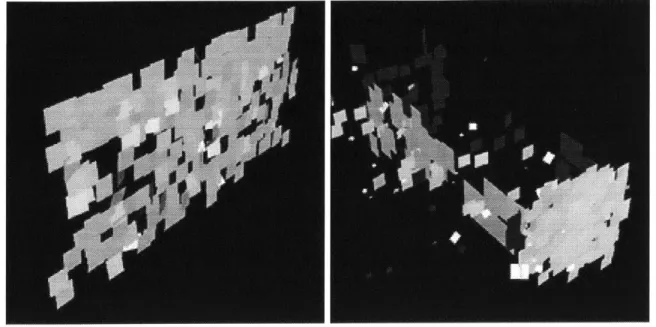
Figure 3.4: Images of Surfels produced by J.P. Mellor's algorithm from the 100 Nodes Dataset. The left image shows the reconstruction of a single facade, and the right image shows Surfels of varying sizes produced for a rectilinear building in Technology Square.
3.1.2 Surfels
In his more recent work with photos from the 100 Nodes Dataset, J.P. Mellor produces Surfels shown in Figure 3.4, which are bits of building surface about ten feet square (but this size may vary within the dataset). He estimates the normal of these surfaces to be accurate to within a couple of degrees. The normal accuracy is much more important with the Surfel dataset than with the Point dataset because the algorithm produces far fewer Surfels than Points. Each Surfel has a small planar Surface to represent its area.
Challenges in dealing with the Surfel dataset include:
" Rejecting outliers and noisy Surfels. In initial datasets, over 50% of the Surfels were outliers (see Figure 3.24), though some of this outlier culling is being done in more recent versions of J.P. Mellor's program.
" Eliminating fencepost problems, where the algorithm is fooled into false correspon-dences by repeated building textures (see Figure 3.5).
" Varying density of the samples.
" Taking advantage of the accurate normals while joining Surfels into larger surfaces which may be planar, spherical, cylindrical, etc.
\\
\
Figure 3.5: Repeated building textures can cause false correlations, a stereo vision fencepost problem. In the reconstruction shown from an early version of J.P. Mellor's algorithm, Surfel evidence at five different plane depths is available for the building facade in the background. The methods for removing Surfels arising from false correlations are described in Section 3.4.4. The techniques for surface creation give special weight to Surfels based on their area and normals.
3.1.3 Edgels
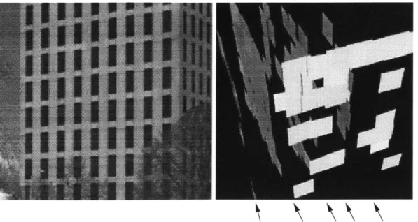
Both Satyan Coorg's and George Chou's algorithms produce line segments which are repre-sented as Edgels in my program (see Figures 3.6 and 3.7). Some of these segments represent geometrical building edges, but many are just features (window and floor delineations) from the texture of the buildings. Edgels are used to neatly border surfaces and indicate where shallow bends in large surfaces should occur. They are also generated by my algorithm at the intersection of two planar surfaces.
Challenges in dealing with Edgel datasets include: " Assigning appropriate weights to each Edgel.
" Identifying spurious Edgels which may bend and crop surfaces incorrectly.
" Making full use of Edgels even though they do not inherently contain any information about the orientation of the surface(s) on which they lie.
Satyan Coorg's method for obtaining Edgels begins with line detection from
Figure 3.6: Horizontal Edgels identified by Satyan Coorg's algorithm from 100 Nodes Dataset and the vertical Surfaces created by projecting these line segments to the ground.
Figure 3.7: Edgels detected by George Chou's algorithm. Spurious Edgels are created when false correspondences are made, but when few images agree with a produced Edgel, its certainty value is low.
tographs and produces possibly hundreds of Edgels per building, while George Chou's al-gorithm produces a much smaller set of Edgels which are averages of many lines detected in the images. The input file parsing modules for each file type must assign reasonable certainty values for Edgels (described in Section 3.4.2) so they can be compared appropri-ately during the Create Surfaces, Match Edgels, and Construct Blocks phases of aggregation described in Sections 3.3.1, 3.3.4, and 3.3.5.
3.1.4 Surfaces
Surfaces are finite, bounded portions of two-dimensional manifolds representing building facades, roofs, columns, domes, etc. Satyan Coorg's algorithm projects clusters of horizontal segments to the ground plane, producing simple rectangular building facades (see Figure 3.6) which are represented as Surfaces in my program. Surfaces are generated by my algorithm to fit clusters of Points, Surfels, and Edgels. For algorithm testing I create synthetic Surface datasets by sampling surfaces in Inventor models (see Section 4.6).
Planar Surfaces are modeled with the equation ax + by + cz + d = 0, which has three degrees of freedom (DOF), and a chain of Edgels to delineate the boundary. Spherical Surfaces are represented with the equation (x - xo)2
+
(y - yo)2 + (z - zo)2 = r2, with four DOF. The system can be extended to include cylindrical Surfaces modeled with two points pi and P2 (representing the endpoints of the cylinder's axis) and a radius r having a total of seven DOF. Constraints on how objects appear in the urban environment can be used to decrease the number of DOF needed to model cylinders. For example, vertical cylinders can be modeled with just five DOF (base point, height, and radius). The system can also represent other types of non-planar surfaces, and clip planes or curved Edgels to specify that only a portion of a sphere, cylinder or other curved surface is present in the environment.Challenges in dealing with Surface Datasets include:
" Discarding very small surfaces and dealing with improper surfaces (those with negative or zero area, or non-convex polygonal outlines).
" Inaccurate normals from poor point cloud surface fitting.
" Ragged edges bounding surfaces generated from clusters of building fragments.
a) * -~- ) *e* c)
a)06 i-- -00 :0b
Figure 3.8: Examples of poorly bordered surfaces: a) Surface which is too big for the evidence because of outliers (shown in gray),
b)
Points which would fit best to a non-convex surface, and c) a set of Point data with a hole in it (the actual surface may or may not have a hole in it).* Determining if a surface has a hole in it (a hole in the data sampling can indicate either a hole in the surface, or the presence of an occluder such as a tree in front of the surface).
* Detecting and correcting Surfaces that are much larger than the majority of the evidence suggests because outliers were included during their construction.
* Varying levels of success in reconstructing surfaces due to an uneven distribution of data samples and variations in data accuracy.
* Modeling non-convex building facade silhouettes.
The tree data structure (described in Section 3.2) organizes objects by location. Data fragments with few neighbors will not. be used to create new Surfaces. The smaller the leaf nodes of the tree, the less likely we are to encounter the oversized surface problems shown in Figure 3.8. Surface density and surface fit criteria (described in Sections 3.4.2 and 3.4.3) are used to identify surfaces which need to be refined or removed. Also, surfaces with very small area relative to the global parameter average.buildingsize can be removed (see also Section 3.4.1). I have chosen to represent only convex surfaces for simplicity of some operations. The system can be extended to manipulate non-convex Surfaces by internally representing them as several smaller convex surfaces.
3.1.5
BlocksBlocks represent buildings and other solid structure in the urban environment and are the final output of the system. I represent a Block as a set of Surfaces which define a closed region of space. The Surfaces are connected to each other through their Edgels in a half-edge data structure which is sketched in Figure 3.9. This structure can represent convex
Figure 3.9: The half-edge data structure provides a consistent method for connecting Edgels and Surfaces into a Block. Every Edgel has a pointer to its twin, next, and previous Edgels and its surface; for example, Edgel El points to E2, E3, E4, and S respectively. Each Surface has a pointer to one of its bordering Edgels; in this example, S points to El. and concave buildings. The vertices may join more than three surfaces.
Challenges in producing and manipulating Blocks include: e Computations with non-convex polyhedral buildings.
e Altering the dimensions and structure of a Block to adapt to new data.
e Modeling buildings composed of both planar and non-planar (spherical, cylindrical, etc.) Surfaces.
Non-convex Blocks are manipulated internally as several convex blocks to make the intersection operations simpler. Each Surface and Edgel that is part of a Block maintains a list of evidence (if any) that led to its creation. If new evidence is added which may modify the conclusions drawn from the original data, the Block is recomputed.
3.2
Build Tree
An enormous amount of data exists within a city, and each building can be sampled to an arbitrary level of detail. Whether we are reconstructing just one building, one block of buildings, or an entire city, we must use a hierarchical system to manage the data. All objects are stored in a three-dimensional k-d tree organized by location to allow fast calcu-lation of each object's nearest neighbors [4]. A k-d tree is a binary tree that is successively split along the longest of its k dimensions resulting in roughly cube-sized leaf nodes. The tree is recomputed automatically as necessary: when new objects are added outside the
bounding box of the current tree, when the data has been modified (to focus on a region of interest, or to remove outliers, etc.), or when global tree parameters have been changed.
When the Build Tree command is performed, either automatically or as requested by the user, any existing tree structure is deleted, a new empty tree is created, and all current objects are added to the tree. The bounding box of this new tree is set to be 10% larger in each dimension than the bounding box of all the objects in the scene. A reconstructed object may have a bounding box which is larger than that of its evidence; the 10% buffer reduces the chance that we will have to recompute the tree because a newly created object's bounding box is also larger than the current tree.
3.2.1 Tree Size and Structure
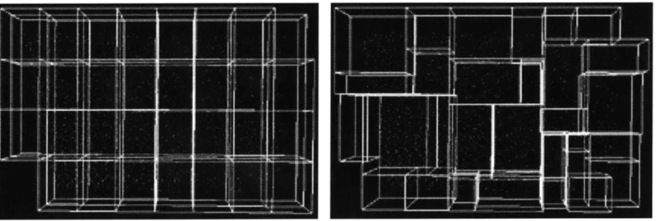
The maximum number of nodes in a binary tree is 2' - 1, where n is the maximum depth. The size of the tree (number of nodes) is critical for performance of the searching operations. A large tree with many leaves will take longer to build and maintain, while a small tree with fewer leaves will require more linear searching through the multiple elements of the leaf nodes. In order to choose an appropriate tree depth, the program needs information from the user about the base unit of measurement of the input data and the desired level of detail for the reconstruction (a single building, a city block of buildings, or an entire city). This information is conveyed with two global parameters: average -building-side, which specifies the dimension of an average size building, and nodes-per-side, which specifies the minimum number of leaf nodes to be used per average building length. For example, if the average -building-side is 500 units and the user requests 2.0 nodes-per-side, the program will divide a scene of size 1000 x 1000 x 500 into 32 leaf nodes as illustrated in
Figure 3.10. The necessary tree depth is computed as shown below, by totaling the number of times each dimension d should be split, where Ad is the size of the tree bounding box in
that dimension.
tree depth =1 + E max(
F
log2 nodesperside x Ad1
0) d=XYZ average building-sideThe user can also specify how each intermediate node of the tree should be split: at the middle of the longest dimension or at a randomized point near the middle of the longest dimension (see Figure 3.11). The randomized option simulates tree structures which might be created by a more complicated splitting function implemented in the future that
1000 unit;S
Figure 3.10: A scene of size 1000 x 1000 x 500 units that has been evenly divided into 32 leaf tree nodes based on the parameters: average building.side = 500 units and nodes-per-side = 2.0. The tree nodes are drawn in grey, and a cube representing an average building is drawn in black.
maximizes the separation of the objects of the node while minimizing the number of objects intersected and required to be on both sides of the split.
The Create Surfaces step of the aggregation algorithm (see Section 3.3.1) is the only phase whose result is directly dependent on the size and structure of the tree. The Refine Surfaces step may further subdivide some leaf tree nodes; the maximum number of additional subdivisions allowed is adjusted by the parameter additional-tree-depth (see Section 3.3.2).
Figure 3.11: Point cloud data set displayed within an evenly split tree and a randomly split tree.
* 0
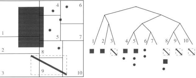
Figure 3.12: Two-dimensional example of how objects are stored in a tree structure. The tree nodes are split at a random point along their longest side until either they have only one object (as for node 1) or the length of each side is small enough (as for node 6). Each leaf node stores the set of all objects whose bounding box at least partially overlaps the node's bounding box. Note that the Edgel is stored in node 8 because its bounding box overlaps the tree node even though the Edgel does not pass through that node. A less conservative method could be used to determine the elements of each leaf node.
3.2.2 Retrieving Nearest Neighbors
Each leaf node of the tree contains a list of all building fragments whose bounding box fully or partially overlaps the tree node (see Figure 3.12). Using this structure, objects may belong to more than one leaf node. When gathering objects from the tree or walking through the tree to perform operations on each element, one must be careful not to double count or process these objects.
Duplicate counting and processing can be avoided by creating a list and verifying with a linear search that each element added is not already in the list. This operation becomes inefficient quickly, O(n2), when creating large unsorted lists of objects. A better choice is to tag elements as they are added to the list and check for that tag when adding new elements, O(n). Also, instead of constructing a list of all the objects (which is costly for large lists of elements), the tree structure can be walked, tagging objects as they are processed. See the Implementation Chapter, Section 4.3 for more details on tagging objects and walking through the tree structure.
The tree structure makes it efficient to collect all objects in a region of space that meet some specified criteria such as object type, whether it was a data or reconstructed element, etc. For example, to conservatively find the nearest neighboring surfaces of an
object, we take that object's bounding box and extend it in each dimension by the relative error distance which is the minimum of the size of the object and the global parameter average building-side. Then we retrieve all leaf nodes of the tree which contain part of the extended bounding box. And finally we identify all Surfaces (being careful to avoid duplicates as described above) in each of these nodes. We are guaranteed to find all objects that could be within the relative error distance from the initial object, but we will probably return others which will be removed by subsequent operations as necessary. With smaller leaf nodes, fewer non-neighbors are returned.
3.3
Phases of Aggregation
The following sections explain the five phases of the aggregation algorithm (shown in Figure 3.1a). These phases may be executed individually by the user through the graphical user interface (described in Appendix B), which has a button for each phase. A sequence of phases to be executed may be specified in a command script (described in Appendix C). The single command Aggregate All executes all five phases.
Surfaces are created and manipulated with the operations Create Surfaces, Refine Surfaces, and Extend Surfaces. These Surfaces are intersected and combined with Edgel data by the operations Match Edgels and Construct Blocks. The intermediate and final results of these steps can be saved for later aggregation sessions or for viewing with other modeling or visualization programs. By default all subphases of the five phases are executed in the order described below; however, each subphase may be disabled (as described in Appendices B and C) for faster processing (for example, it may be known that there are no quadric surfaces) or for inspection of intermediate results. The final results are not dependent on the order of phase or subphase execution, but it is more efficient to run certain phases first (for example the subphase Extend Excellent Surfaces should be run before Extend All Surfaces).
The phases of aggregation create new objects called reconstructed objects which can be modified unlike data objects which are never modified. Data objects are deleted only if they are malformed (too small or non-convex, etc.), are outliers as detailed in Section 3.4, or are outside the region of interest. Each reconstructed object stores pointers to its evidence (objects that were used to create it) and each object stores pointers to any
reconstructed objects to which it contributes. Section 3.4 details several important metrics: relative weight, evidence fit, surface density, and surface fit.
3.3.1 Create Surfaces
In this phase, the program creates Surfaces to best fit Point, Surfel, and Edgel data which has been sorted into tree nodes. The computation focuses on Points, but Surfels and Edgels are incorporated with special weights. For leaf nodes with a minimum number of data objects (specified by parameter tree-count), the algorithm computes a best fit plane using an iterative least squares technique similar to that used by Fua [13] and Hoppe et al. [15]. The Extend Surfaces phase will fit objects to non-planar Surfaces as appropriate.
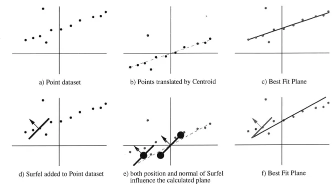
Fitting a Plane to a collection of Points
Each iteration of the plane fitting algorithm proceeds as follows: The centroid C = (Xc, Yc, ze) is calculated to be the weighted average of the Point positions Pi = (xi, yi, zi). For the first iteration wi (the weight of Point i) = relative weighti. In subsequent itera-tions wi = relative weighti x evidence fits to p, where p is the best fit plane from the previous iteration. The metric relative weight is described in Section 3.4.2 and evidence fit is described in Section 3.4.3. The n positions P are gathered into a 3 x 3 matrix M:
M = wi((Pi - C) x (Pi - C)) i=1
The values for the coefficients of the plane equation ax + by + cz + d = 0 are calculated by finding the eigenvector associated with the largest real eigenvalue A of matrix M:
a a
M b = A b
c c
The positions Pi were translated by the centroid C so the best fit plane passes through the origin (0, 0, 0) and the coefficient d for the calculated plane is zero. d is calculated for the original positions as follows:
d = -(axc + byc + czc)
The above steps are shown in Figure 3.13 a, b, and c. The number of iterations performed can be adjusted by the global parameter surface-iterations. Fua [13] found that three to five iterations were optimal.
0 0 0 0 9 0 0 0 0 0 5-C-Ir a) Point dataset 0 e d0 Surfe _ _
d) Surfel added to Point dataset
40 0
S
. -~0
0--b) Points translated by Centroid
,0 5- I
e) both position and normal of Surfel influence the calculated plane
c) Best Fit Plane
f) Best Fit Plane
Figure 3.13: Two dimensional example of how to fit a line to a Point and Surfel dataset. a and d show the original objects. In b and e the objects are translated so their centroid is at the origin and c and
f
show the final planes. In e, the Surfel is shown translated in two ways: first it is translated with the other objects and is drawn with a large black dot for the center of mass, the other is drawn at the origin and shows two black dots which influence the normal of the final surface. Note that the Surfel's normal does not fit the plane very well, so in subsequent iterations the Surfel will be given less influence over the plane created.Incorporating Surfels and Edgels
A Surfel's position can be treated like a Point in the above algorithm, but its normal needs special consideration. In addition to adding the Surfel's position into the matrix M we add four additional points each one unit away from the origin in the plane perpendicular to the normal.
Po = Surfel center of mass
v, = any unit vector I to Surfel normal
V2 = the unit vector I to Surfel normal and vj
P1 = di P2 = V2
P3 =-V1
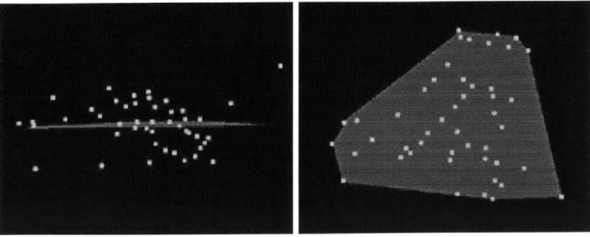
Figure 3.14: A collection of Points from a node of the tree and the convex hull of each Point's projection onto the best fit plane.
P4 = -V2
relative weights.rfel
wo = 2
relative weightsfl
W 1 =w 2 =Ws=W4 = 8
For example, if the Surfel's normal is (0, 0, 1), we add the points (1, 0, 0), (0, 1, 0), (-1, 0, 0), and (0, -1, 0). A two-dimensional example is shown in Figure 3.13 d, e, and
f.
Edgels are incorporated into the plane computation described above by simply adding the endpoints of the Edgel to matrix M:
Pi = Edgel endpoint1 P2 = Edgel endpoint2
relative weightEdgel
wl=W2 = 2
Determining a Boundary
Once a plane has been estimated for each tree node having a minimum number of data elements, a bounding outline for the Surface is found by projecting the elements of the tree node onto the new plane and computing the convex hull of those two-dimensional points as shown in Figure 3.14. Objects that poorly fit the computed plane are not used in computing this boundary. The final orientation of the Surface (which side is the "front") is determined by computing the weighted average of the normals of all evidence contributing to the surface.