A method for classifying and comparing non-linear trajectories of ecological variables

HAL Id: hal-03051861

https://hal.umontpellier.fr/hal-03051861

HAL is a multi-disciplinary open access archive for the deposit and dissemination of sci-entific research documents, whether they are pub-lished or not. The documents may come from teaching and research institutions in France or

L’archive ouverte pluridisciplinaire HAL, est destinée au dépôt et à la diffusion de documents scientifiques de niveau recherche, publiés ou non, émanant des établissements d’enseignement et de recherche français ou étrangers, des laboratoires

A method for classifying and comparing non-linear

trajectories of ecological variables

Stanislas Rigal, Vincent Devictor, Vasilis Dakos

To cite this version:

Stanislas Rigal, Vincent Devictor, Vasilis Dakos. A method for classifying and comparing non-linear trajectories of ecological variables. Ecological Indicators, Elsevier, 2020, 112, pp.106113. �10.1016/j.ecolind.2020.106113�. �hal-03051861�

A method for classifying and comparing non-linear trajectories of ecological variables Stanislas Rigal1_{*, Vincent Devictor}1_{, Vasilis Dakos}1_.

1_{ISEM, Univ Montpellier, CNRS, EPHE, IRD, Montpellier, France.}

*Corresponding author, email: stanislas.rigal@umontpellier.fr Abstract

Temporal dynamics in ecological variables are usually assessed using linear trends or smoothing methods. Those trends qualitatively summarise the increase or decrease in the variable of interest over a given time period. Yet, linear trends do not capture changes in the direction or in the rate of change of indices such as population trajectories, that may typically occur when conditions improve or worsen following conservation actions or environmental disturbances. In a similar way, non-linear methods while aiming to fully characterise population trajectories, fail to end up with a standard classification. Here, we propose and test a simple method to classify the trajectory of a given ecological variable according to its trend and acceleration. Our method is based on fitting a second order polynomial that is used to describe a trajectory according to its direction, velocity, and curvature (accelerated or decelerated). We apply this method to the temporal dynamics of bird populations monitored by the French Breeding Bird Survey as a case study. Using data for more than 100 species monitored from 1989 to 2017 in more than 2000 sites, we show that one quarter of the studied species have dynamics that can be better described by our polynomial approach than typically-used linear analysis. We also show how it can be used to analyse indicators constructed with multi-species indices. Our method can be applied to any type of ecological variable either to classify trajectories of ecological variables in time or trajectories of ecological variables across pressure gradients. Overall, our results suggest a more systematic investigation of non-linear trajectories when analysing the dynamics of ecological variables.

Key-words: bird, conservation, ecological variables, non-linearity, polynomials, population dynamics, trend analysis.

1. Introduction

As biodiversity is undergoing a major decline (Ripple et al., 2017), international initiatives have set several ambitious targets to combat this trend, by protecting species and habitats or maintaining and restoring ecosystems (CBD, 2010; EC, 2011). These objectives require the development of relevant data and statistical tools to estimate any progress towards those targets.

Different types of variables has been proposed for measuring the “changing state of nature”. For instance, a suite of “biodiversity variables” have been proposed to detect critical biodiversity 1 2 3 4 5 6 7 8 9 10 11 12 13 14 15 16 17 18 19 20 21 22 23 24 25 26 27 28 29 30 31 32 33 34 35 36 37 38 39

changes (Schmeller et al. 2018). Whatever the ecological level considered (species, habitat, ecosystem) and the specific definition used (variable, indices, indicator), detecting changes in the dynamics of biodiversity responses is key to temporal ecology and conservation policy (Wolkovich

et al., 2014). Among possible approaches, the analysis of temporal trends in populations of habitat

specialist species (e.g. farmland birds, Gregory et al., 2005), or in aggregated indicators of population dynamics (e.g. Living Planet Index, Loh et al., 2005) has become common practice for monitoring human impact on biodiversity (Vačkář et al. 2012).

Ideally, an improved biodiversity status should be revealed by a switch from a decrease to an increase (or at least to a stabilisation) in the temporal trend of those indices (Donald et al., 2007; Koleček et al., 2014; Sanderson et al., 2016; Koschová et al., 2018). More generally, the aim of calculating temporal trends is to describe the state of a given variable with regard to its past with a straightforward descriptor that can be easily interpreted and used in further analysis (e.g. to compare dynamics between species or to relate the trend in the variable to specific pressures).

However, the term "trend" creates confusion about what is measured when a statistical model is fitted to a trajectory (i.e. a time series) of a given variable of interest. The trend is usually measured after fitting a linear model that estimates the average rate of change of the variable over a given period (Link and Sauer, 1997a) and it is used to describe the trajectory. When estimating a trend, however, one only synthesises the overall change in terms of direction (the sign of the trend), and steepness (the magnitude of the trend). Yet, a trajectory is more than its trend as it is defined by the pattern of fluctuation itself. When studying a trajectory, the purpose should rather be to find the most accurate description of changes over time in terms of direction, velocity, curvature, or even the timing of such changes. Surprisingly, trends and trajectories are not always separated in the study of ecological variables (Humbert et al., 2009; Inger et al., 2014).

Relying on linear trend methods or on a percentage of change between the first and last values remains largely dominant in classifying and comparing temporal changes in population dynamics for most of the well-studied groups, such as birds (Julliard et al., 2004; Donald et al., 2007; Reif, 2013; Inger et al., 2014; Heldbjerg et al., 2018; Rosenberg et al., 2019), fish (Christensen et al., 2014; Vasilakopoulos et al., 2014), and insects (Hallmann et al., 2017; Lister and Garcia, 2018; Sánchez-Bayo and Wyckhuys, 2019). But focusing either on trends or trajectories can lead to different interpretations as numerous population dynamics are non-linear (Clark and Luis, 2019) . Before any qualitative change of a given variable can be detected, the trajectory of the variable can adopt different shapes with specific meanings that cannot be captured by simply measuring the trend. For instance, for a population trajectory reflecting the conservation status of a threatened 40 41 42 43 44 45 46 47 48 49 50 51 52 53 54 55 56 57 58 59 60 61 62 63 64 65 66 67 68 69 70 71 72 73 74 75

species, the deceleration of the decrease already reveals a better situation (Fig. 1A). On the contrary, an accelerated decrease mirrors a stronger degradation (Fig. 1B). Thus, the variation in the rate of change along the trajectory is highly informative from a conservation perspective and yet cannot be entirely captured by a linear trend approach. Worse, linear trends can mask reversal dynamics, a concave or convex hump shaped curve that is typically qualified as “stable” by a linear model (Fig. 1C). Therefore, studying complete trajectories beyond simple trends is crucial to track the improvement or failure in conservation policies as well as to identify changing points that may follow the implementation of a conservation policy.

A plethora of other than linear methods to describe population trajectories is already available (Thomas, 1996; Link and Sauer, 1997b; Ruppert et al., 2009; Dornelas et al., 2013; Tittensor et al., 2014). Most of these methods rest on generalised linear models with polynomial regression splines (Cunningham and Olsen, 2009) or generalised additive models (GAM) (Fewster et al., 2000; Buckland et al., 2005). Although these methods are fundamental to fit and describe complex non-linear dynamics, the details of such complex shapes can be irrelevant for assessing the status of a population trajectory and difficult to use for comparison between different species. The reason is that in these non-linear models, the type of function used and the degree of freedom allocated to the corresponding statistical models are often not a priori constrained by the user (otherwise it would correspond to a parametric case (Brun et al. 2019)) but rather adjusted to the data. This leads to difficult interpretations as the risk of overfitting increases compromising the comparison between datasets. For instance in a GAM, smooth functions are built on a trade-off between the smoothness of the function and the fidelity to the data which implies a selection (either by generalised cross validation or marginal likelihood) of the smoothing parameters (Wood, 2017). Alternatively, simple non-parametric methods also exist (e.g. correlation rank (Yue and Wang, 2004; Sonali and Kumar, 2013; Adarsh and Janga Reddy, 2015)), but they remain highly conservative in detecting no more than a dominant trend. Other methods identify breakpoints along a trajectory, for instance by fitting segmented relations usually through piecewise regression models (Muggeo, 2003; Muggeo, 2008; Fong et al., 2017), or by applying sequential or iterative regime shift analysis methods (Rodionov and Overland, 2005; Gröger et al., 2011). Although these techniques help to locate abrupt changes along a trajectory, they do not synthesise the trajectory beyond identifying particular changing points.

Overall, the current approaches to study and compare non-linear trajectories in ecological variables do not offer a simple method for classifying trajectories based on their general shape. Such a method should be flexible enough to handle most ecological data, it should use simple statistical 76 77 78 79 80 81 82 83 84 85 86 87 88 89 90 91 92 93 94 95 96 97 98 99 100 101 102 103 104 105 106 107 108 109 110

estimates to classify trajectories, and these estimates should be easy-to-use for comparing different trajectories. We suggest that a method that meets these criteria could include: a) estimating the direction of change of a trajectory, b) estimating the rate of change of a trajectory, c) identifying whether the rate of change is accelerating or decelerating within a trajectory, and d) detecting points where the direction of change of a trajectory switches sign. Such a method would not reject linear trend analysis nor replaces GAM-like approaches, but would rather aim at providing a simple and generic classification of non-linear trajectories.

In this paper, we develop such a generic method to classify trajectories of any ecological variable (population indices, multi-species indicators or any kind of temporal series) according to their direction (decline, increase, stable) as well as to their overall shape (accelerated, decelerated, convex or concave). We describe this method step-by-step and we test it in simulated trajectories that resemble typical time series of monitored populations. We further show how and why this method could be used in two empirical examples. We use population dynamics of the 108 most common species monitored by the French Breeding Bird Survey (FBBS) from 1989 to 2017 (Jiguet

et al., 2007) to illustrate how our method can be used to describe the conservation status of these

populations. We finally apply this method on multi-species indicators (MSI) for farmland and woodland birds. We anticipate that this method will be sensitive to well identified pitfalls of classical monitoring programs (Buckland and Johnston, 2017) that might have a particular incidence on the uncertainty of the variable of interest resulting in a wider sampling error. A method accounting for this sampling error has been recently proposed for multi-species indicators (Soldaat

et al., 2017). We therefore adapted this method to take into account sampling error in our method

when it is available. We also tested the sensitivity of our method to critical methodological choices or change in data quality. We highlight the advantages and disadvantages of our approach by comparing our results to those estimated by most common linear methods.

2. Materials and methods

2.1 A general classification of trajectories for ecological variables

We use the properties of a second order polynomial function to describe and classify the overall shape of any trajectory.

Let Y be a quantitative discrete or continuous variable (e.g. population abundance or any ecological variable) and X a quantitative continuous variable representing time (year, month or days). The characterisation of a second order polynomial function can be achieved in two steps (Fig. 2A): Step 1. We first fit a second order polynomial between Y and X through a least-square regression: 111 112 113 114 115 116 117 118 119 120 121 122 123 124 125 126 127 128 129 130 131 132 133 134 135 136 137 138 139 140 141 142 143 144 145 146 147 148

Y =α0+α1X +α2X2 (1)

Such a regression model performed using orthogonal polynomials removes the correlation between the first (X) and the second order (X²) variables (Narula, 1979). The significance of each coefficient (α1 for first order and α2 for second order) is therefore used to test whether the second order

significantly improves the regression compared to the first order. More precisely, a second order polynomial (Eq. 1) can discriminate between a stationary process (if α1 and α2 are not significant), a

monotonous process (if only α1 is significant), and an accelerated process (if α2 is significant).

We fit this function within the interval bounded by X0 and XT, respectively the first and last values

of X, to generate a curve that can be either convex ( ) or concave ( ) (Fig. 3). For a convex curve,_{⋃ ⋂} this interval on which the function is fitted necessarily delineates one of the following cases: a decelerated decline (Fig. 3A.1), a convex phase (Fig. 3A.2) or an accelerated increase (Fig. 3A.3). For a concave case three analogous cases can be described: a decelerated increase (Fig. 3B.1), a concave phase (Fig. 3B.2), or an accelerated decline (Fig. 3B.3).

Step 2. We then characterise the fitted polynomial function with simple metrics, i.e. we transform the information contained within the function and the interval into a readable description using the direction, the acceleration, the velocity and the changing points of the trajectory (Fig. 2-3). The direction of the trajectory is defined as being either a decline, nil or an increase. The acceleration corresponds to an accelerated, constant, or decelerated phase when the direction is either a decline or an increase, or refers to a convex, stable or concave phase when there is no direction (Fig. 2). Moreover, the velocity represents the rate of change of a given trajectory and the changing points designate where the rate of change of the trajectory adopts a different profile (Fig. 3).

For linear cases (α2 non significant), Y becomes a linear function of X (i.e. Y = α0+α1X). The four

indices are completely determined by the sign and the magnitude of the slope (α1). The direction is

an increase, nil, or a decline for positive, null, or negative slopes respectively. The acceleration is null, the velocity is the magnitude of the slope and there is no specific point of noticeable change that can be identified.

149 150 151 152 153 154 155 156 157 158 159 160 161 162 163 164 165 166 167 168 169 170 171 172 173 174 175 176 177 178 179 180

For non-linear cases (α2 significant), a standardised classification should be able to discriminate

between decelerated or accelerated cases and convex, stable or concave dynamics (Fig. 3). This is done as follows:

Direction. To qualify the behaviour of the function over a given period, we use the direction of the function around the centre Xm of the interval [X0, XT] (corresponding to the whole time series

length). The direction of Y is then determined by the sign of the slope of the tangent TXm given by

the linearisation around Xm:

T_Xm(X )= ˙Y

₍

_{) (}

₎

₍

₎

where Ẏ(Xm) is the first derivative of Y:

˙Y

(

)

Ẏ is computed around Xm both at Xm-δ and Xm+δ (Fig. 3), where δ is equal to 25% of the interval

[X0, XT]. As the direction can change only once along a second order polynomial, if this

modification does not happen on [Xm-δ, Xm+δ], it implies that the change occurs either on ]-∞, Xm-δ[

or on ]Xm+δ, +∞[. If it occurs on ]-∞, Xm-δ[, the direction is constant on [Xm-δ, XT] and by symmetry,

if the change happens on ]Xm+δ, +∞[, the direction is constant on [X0, Xm+δ]. In both cases, the

direction stays the same on at least 75% of the interval [X0, XT] and we assume this direction

accurately reflects the main direction of Y on [X0, XT]. In these cases, if Ẏ(Xm-δ) > 0 and Ẏ(Xm+δ) >

0, the direction is an increase and if Ẏ(Xm-δ) < 0 and Ẏ(Xm+δ) < 0, the direction is a decline. If the

sign of Ẏ changes on the interval [Xm-δ, Xm+δ], it means that Ẏ becomes zero around Xm and hence

the direction is considered as nil and there is no alternative possibility.

Acceleration. The acceleration of the polynomial fit on the interval is given either by the sign of the second order coefficient α2 or by the sign of γγ, the derivative of the curvature function γ (Eq. 4)

(O’neill, 2006). This choice depends on whether the direction is nil (sign of Ẏ(Xm-δ) ≠ sign of

Ẏ(Xm+δ)) or not. 181 182 183 184 185 186 187 188 189 190 191 192 193 194 195 196 197 198 199 200 201 202 203 204 205 206 207 208 209 210 211

˙γ

(

)

₍

)

(

(

₎

)

When the direction is nil (Fig. 3 A.2, B.2), the acceleration refers to the convexity or concavity of the trajectory and only the sign of α2 is needed to describe it (convex for α2 > 0, concave α2 < 0).

When the direction is an increase or decline (Fig. 3 A.1, A.3, B.1 and B.3), the acceleration cannot be described solely by the sign of α2, because whether the function is in an accelerated or

decelerated phase depends on the interval which is regarded. For instance, if α2 > 0, we could have

a decelerated decline (Fig. 3A.1) or an accelerated increase (Fig. 3A.3) depending on the interval considered. We therefore introduce a criterion that directly refers to the curvature γ of the function irrespective of the interval (Fig. S1). This criterion is given by computing γγ the first derivative of the curvature function γ at Xm the centre of the interval [X0, XT] (Eq. 4) (supplementary materials 1

for calculation details).

When the interval is on the left side of the minimum or maximum of the second order polynomial, whatever the sign of α2, the function is decelerating (Fig. S1). When the interval is on the right side

of the minimum or maximum, the function shows an acceleration. The sign of γγ is the opposite when the sign of α2 changes. By multiplying the sign of γγ by the sign of α2, we obtain a consistent

type of acceleration for the variable considered (Y). When this sign is negative, it corresponds to an acceleration and when it is positive, it corresponds to a deceleration.

Velocity. The velocity is given by the magnitude of the tangent at Xm, i.e. the value of Ẏ(Xm) (Eq. 3).

The velocity can be compared between two curves only if they belong to the same type of trajectories. For instance, it would not make sense to compare the speed of a decelerated trajectory (Fig 2B case 9) with the speed (slope) of a linear increase (Fig 2B case 6).

Changing points. Non-linear or multiple linear regression methods can provide changing points or periods (Buckland et al., 2005; Fewster et al., 2000; Muggeo, 2003; Cunningham and Olsen, 2008; Smith et al., 2015). Here, for each second order polynomial curve three local points of interest can be identified in theory. Those points correspond to values of X where a shift in the rate of change is observed. No significance test is required as the significance of the second order polynomial implies the existence of these points (but see below for standard deviation). The first point (p1) marks the

212 213 214 215 216 217 218 219 220 221 222 223 224 225 226 227 228 229 230 231 232 233 234 235 236 237 238 239 240 241 242

minimum (for convex cases) or maximum (for concave cases) of the polynomial curve and corresponds to the value of X when Ẏ is zero (Eq. 5). The two other points (p2 and p3) delineate the

values of X where the rate of change is mainly driven by a horizontal or vertical component (Eq. 6) (see supplementary material 2). In practice, among these three points (p1, p2 and p3), only the ones

which fall within the interval [X0, XT] are generally relevant (Fig. 3). These points only serve as

potential changing points in the overall shape of trajectories and need to be interpreted as such by the user.

{

₍

₎

(

)

{

₍

₎

₍

₎

{

In many cases, the sampling error of the Y value is also accessible and needs to be considered to estimate Y uncertainty. We therefore use a Monte Carlo simulation method to account for this sampling error (SE) adapted from Soldaat et al. (2017). We first set the Y value for the reference year (baseline year that can be either the first, last or central year or a specific year chosen by the user) to 100 and any Y value below 1 is truncated to 1 and its SE set to 0. We then log-transformed the Y values and we applied the Delta-method (Agresti, 2002) to obtain the sampling error of Y on a log scale (SElog(Y) = SE(Y)/Y). 1000 Y vectors are then simulated by taking values from a normal

distribution with a mean equal to the log-transformed Y values and the standard deviation equal to the SElog. Each Y vector is back-transformed to the original Y scale, the reference year value is set to

100 and other values are expressed as a percentage of the value of the reference year. We then classify each simulated Y after estimating its acceleration, velocity and potential changing points. As simulated trajectories may be classified in different classes, we perform a binomial (if two different classes) or multinomial (if more than two different classes) test to assess the significance of the predominant class. If both a non-linear and a linear class are predominant but none of them significantly, Y is classified as belonging to the linear class. Only the simulations belonging to the selected class are kept and used to calculate the average velocity and the average changing points (if any) and their standard deviation.

243 244 245 246 247 248 249 250 251 252 253 254 255 256 257 258 259 260 261 262 263 264 265 266 267 268 269 270 271

In summary, using the classification method described above (Fig. 2A), one can classify any trajectory as belonging to only one of the nine classes: accelerated decline, constant deccline, decelerated decline, concave, stable, convex, decelerated increase, constant increase and accelerated increase (Fig. 2B). The direction and the type of acceleration are enough to cover this classification which is obtained unambiguously because both the direction and the acceleration are retrieved from the statistical significance of the second order polynomial coefficients. Moreover, two additional properties can be easily obtained, namely the velocity of the change, and potential changing point(s) with a significant shift in the rate of change of Y. The classification being based on trajectories in a given interval [X0, XT], it is by definition dependent on the time interval considered. The

incorporation of the sampling error allows to test the significance of the classification and to give an estimate of uncertainty (as standard deviation) for velocity and potential changing points.

2.2 Sensitivity to time series length, missing data, noise and sampling error

We tested the sensitivity of the proposed method on simulated trajectories that mimic each of the nine classes (Fig. 2B). To produce time series we used the second order polynomial (Eq. 1) with parameter values α1 and α2 chosen to be close to the coefficients obtained from empirical time

series and selecting only the part of the produced parabola that resembled the nine classes (for details see supplementary material 3). We performed a sensitivity analysis to four potential sources of biases (see supplementary material 4). First, we explored the effect of the time series length. Second, we explored the effect of gaps in the monitored data as typically the frequency of monitoring can differ from year to year. Third, we explored the effect of process noise (Dennis et

al., 2006) as additional year-to-year variation on the trend. Noise corresponds to a deviation from

the process and it influences the position of the Y value for a given X value. Finally, we explored the effect of sampling error due to incomplete sampling, weaknesses in detectability or misidentification of species. Sampling error corresponds to a dispersion metric of uncertainty of a Y value for a given X value.

2.3 Classifying trajectories of empirical ecological variables: an illustration using bird populations We tested our method on an empirical dataset. We classified bird population time series from the French Breeding Bird Survey (FBBS) from 1989 to 2017. To be validated by the FBBS, volunteer ornithologists had to follow a standardised protocol on fixed sites (2693 since 1989) on which a fixed number of point counts were carried out by the same observer in the same order. Each point 272 273 274 275 276 277 278 279 280 281 282 283 284 285 286 287 288 289 290 291 292 293 294 295 296 297 298 299 300 301 302 303 304 305

count of each site is monitored twice a year during the same period (5 or 15 minutes) 1 to 4 hours after sunrise, between 1st of April and 15th of June to take into account early and late breeding birds. Of the 242 species recorded in the dataset, we selected the most abundant species (99% of the total abundance) to restrict our analysis only to the most common species, easy to observe and less exposed to sampling biases. After removing non-selected species and sites only monitored once, our dataset comprised 2144 sites and 108 species (supplementary materials 5). For each site and species, count data from all the points of each given site were summed (after taking the maximum of the two monitoring spring sessions for each point) as a proxy for the local abundance of the species in a given site and a given year.

Note that many ecological data are similar to what is collected by the FBBS, i.e. they use multi-species and multi-sites surveys to derive yearly variations in the abundance of each multi-species or in more elaborated indicators combining multi-species indices (Loh et al., 2005; Pereira and Cooper, 2006; Butchart et al., 2010; Inger et al., 2014).

We thereafter applied our method to yearly population indices (see supplementary materials 6) of each of the 108 species from the FBBS during the period 1989-2017 corresponding to [X0, XT],

using 2001 as the reference year. For each species i, the yearly index (Yi) was considered as the

response variable (Y) and years as polynomial explanatory variable (X) (Eq. 1).

Finally, we also tested our method on multi-species indicators (MSI) rather than individual species. MSI are typically used to capture the general trend of a specific group of species of interest (e.g. farmland birds). To compile these MSI, we selected farmland and woodland specialist species (MNHN, 2019).

All analyses were performed in R (version 3.4.4). Bird data were obtained from the French National Natural History Museum in 2018. A workflow of the proposed method is available as Rmd file and can be downloaded at https://github.com/StanislasRigal/classtrajectory.

3. Results 3.1 General case

Testing our method on the simulated trajectories, we were able to correctly classify between 44.6% and 98.3% depending on the biases considered (Table 1). In terms of sensitivity to time series 306 307 308 309 310 311 312 313 314 315 316 317 318 319 320 321 322 323 324 325 326 327 328 329 330 331 332 333 334 335 336 337 338 339 340

length, we found that the classification was weakly sensitive to the length with a slightly better classification percentage for longer time series (Table 1). 96.8% of the simulations were correctly classified, when the time series length was 30, which is the time series length covered in the empirical example. This percentage is not significantly different from the percentage obtained for length equal to 70 (binomial test p-value = 0.156) but it was significantly higher than the percentage obtained for a length equal to 10 (binomial test p-value < 0.0001). The highest percentage was found for a length of 50 but it was not significantly higher than the percentage found for a length of 70 or 90 (binomial test p-value = 0.127 and 0.331). Overall this source of bias has less impact on the percentage of correct classifications than others. The average distance between expected and observed potential changing points was around 5 or 6% of the time series length. For missing data, we found that the more the data are complete (the more the ratio between monitored years and time series length is close to 1), the more the classifications were correct, with a maximum of 96.8% of correct classification for a complete time series (ratio = 1). For noise and sampling error, we found that these biases generated the most high percentage of misclassification.

Time series length (Years) (ratio of missing data =

1, noise = 5%, sampling error = 5%) 10 30 50 70 90

Correct classifications (%) 90.3 96.8 98.3 97.5 97.8

Mean relative distance from observed to simulated

changing points (% of time series length) 4.9 5.0 5.5 5.8 6.3 Missing data (Ratio between monitored years and

time series length) (time series length = 30, noise = 5%, sampling error = 5%)

0.2 0.4 0.6 0.8 1

Correct classifications (%) 48.8 59.7 72.5 82.8 96.8

Mean relative distance from observed to simulated

changing points (% of time series length) 3.8 3.7 3.6 3.8 5.0 Noise (% of Y range) (time series length = 30, ratio

of missing data = 1, sampling error = 5%) 5 15 25 35 45

Correct classifications (%) 96.8 82.4 63.3 48.9 44.6

Mean relative distance from observed to simulated

changing points (% of time series length) 5.0 9.5 12.1 16.1 17.9 Sampling error (% of Y range) (time series length

= 30, ratio of missing data = 1, noise = 5%) 5 15 25 35 45

Correct classifications (%) 96.8 85.6 56.8 54.8 51.7 341 342 343 344 345 346 347 348 349 350 351 352 353 354 355

Mean relative distance from observed to simulated

changing points (% of time series length) 5.0 8.6 7.7 8.6 10.2 Table 1: Averaged percentages of correct classifications for each value of each source of bias. The time series length is expressed in years. The ratio corresponds to the number of monitored time steps to number of time steps. The process noise and the sampling error are expressed in percentage of the Y range (Ymax-Ymin).

3.2 Case-study

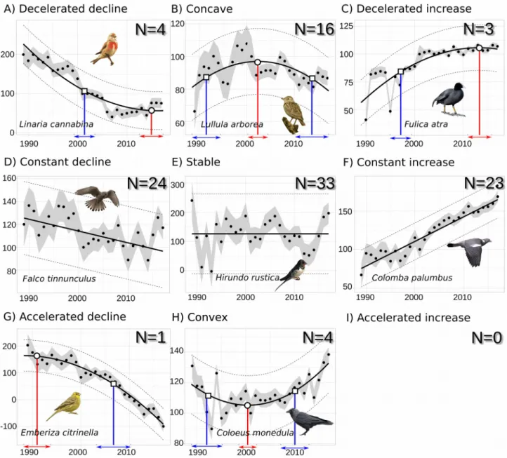
We applied our classification method on bird population trajectories recorded in France from 1989 to 2017. We found that among the 108 species trajectories, 80 were linear while for the other 28 (i.e. 26% of the 108 trajectories) a second order polynomial was better than the linear fit. 26 species trajectories were classified as increase of which three were decelerated and 23 constant (Fig. 4 F, I). 29 species trajectories were classified as decline of which four were decelerated, 24 constant and one accelerated (Fig. 4 A, D, G). 53 species trajectories were neither classified as decline nor as increase, of which four were convex, 33 remained stable and 16 had concave dynamics (Fig. 4 B, E, H).

We also quantitatively compared trajectories based on their velocity. Note that the velocity was not recorded when the trajectory direction was nil (concave, stable or convex classes) as it would have been null. Also no velocity was calculated for the accelerated increase class as we found no species belonging to this class. We found that species from the same class can differ greatly in velocity. For instance, between two decelerated and decling species, Pica pica had a velocity three times greater than Corvus frugilegus (respectively -8.4 and -3.0) depicting a stronger decrease of Pica pica relative to Corvus frugilegus. Note that the comparison of species velocities for trajectories belonging to different classes is not meaningful. For instance, the velocity of Emberiza citrinella, an accelerated and declining species, is similar to the velocity of Pica pica, a decelerated and declining species (respectively -9.2 and -8.4). The trajectories of those two species being different, their velocities cannot be compared although they are quantitatively similar. This highlighted the need of considering the trajectory class before conducting velocity comparisons and more generally the need of caution when performing linear trend comparisons.

For some cases, we also detected potential changing points that depict either a change from an increase to a decline (or vice versa), or an acceleration or deceleration of the rate of change. For 356 357 358 359 360 361 362 363 364 365 366 367 368 369 370 371 372 373 374 375 376 377 378 379 380 381 382 383

instance, Emberiza citrinella started to strongly decrease in 2007 (p2, sd = 1.9, Fig. 4A). During the

same period, Coloeus monedula slowed down its decline in 1991 (p2, sd = 2.5), reached a minimum

in 2000 (p1, sd = 0.9) and mainly increased after 2010 (p3, sd = 1.3) (Fig. 4B). These points can

provide additional information on each species dynamics of potential conservation interest such as population responses to pressure or conservation changes.

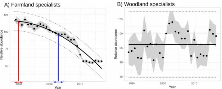
Using our method on MSI, we found a significant accelerated decline in farmland specialists (Fig. 5A) (α2 = -0.08, α1 = 300, sd = 7.06, p-value < 0.0001). In contrast, we found a stable trend in

woodland specialists (slope = 0.09, sd = 5.9, p-value = 0.28) (Fig. 5B). 4. Discussion

In this paper, we showed how trajectories of ecological variables can be classified into nine classes using a method that is simply based on fitting a 2nd _{order polynomial model (Fig. 2). Our method}

basically dissects the dominant shape of a trajectory into 2 properties: the direction and the acceleration. In addition, this method can indicate the velocity and potential changing points along the trajectory where a shift in the rate of change happens. As such, our approach helps to provide comparable and easy-to-use information that goes beyond the current classification and comparison method based on linear trend analysis or percentage of change (Vorisek et al., 2010; Inger et al., 2014).

When applied to empirical population trajectories, we showed how this method gives additional information on species dynamics compared to common linear approaches. Studying linear trends of our empirical example would have masked significant non-linear dynamics for more than 25% of the studied species between 1989 and 2017. Thus, using a common linear approach no distinction could have been found between species with stable trajectories and those with convex or concave dynamics, compared to fitting a second order polynomial function. Moreover, decreasing or increasing trends would only have been differentiated quantitatively using velocity whatever their individual shapes. Finally, potential changing points would have been inaccessible using a unique linear regression although they can be provided using other methods (Fewster et al., 2000; Muggeo, 2003; Cunningham and Olsen, 2009; Smith et al., 2015). These remarks also stand for the multi-species indicators analysed in this study. The dynamic of the forest multi-species MSI was classified as stable and other non-linear methods may be then applied to more precisely fit the narrow range variations. The dynamic of the farmland species MSI was categorised as an accelerated decline. 384 385 386 387 388 389 390 391 392 393 394 395 396 397 398 399 400 401 402 403 404 405 406 407 408 409 410 411 412 413 414 415 416 417

Therefore, beyond the now well-described decline in farmland birds (Donald et al., 2001; Gregory

et al., 2019; Newton, 2004; Reif and Vermouzek, 2019), their decrease was even faster between

1989 and 2017 in France. Of course, an analysis restricted to a different interval, like for instance focused on the last years (showing a stabilisation), would have led to a different classification. Thus, it should be clear that the classification given by this method synthesises the shape of the trajectory over the whole available time series. In that sense, different dynamics during a particular part of the trajectory may be explored by applying the method to a specific period.

The presented method can also be used to search for signs of improvement following, for instance, large-scale conservation policies. As pressures on ecosystems are not intrinsically supposed to be linear it may be relevant to combine this method to synthetically describe population trajectories along with non-linear dynamics of pressures that are experienced by species in different areas (e.g. to test whether the trajectories of ecological variables and of candidate pressures are similar (in shape) and synchronous (via the changing points)). Previous studies have selected a given year (often close to a new conservation legislation enforcement) to compute before/after linear trends or linear approximations (Donald et al., 2007; Mace et al., 2010; Koleček et al., 2014; Sanderson et

al., 2016). Our method does not require the selection of a particular year. Rather, it can

independently highlight specific points where trajectories change in direction, which can be used for evaluating a potential temporal lag between legislation and biodiversity responses (Male and Bean, 2005).

The classification method we propose is sensitive, to some extent, to the length of the time series, the data resolution, the magnitude of noise (distance to the process influencing the position of a value) and the importance of sampling error (dispersion metric corresponding to the uncertainty of a value). The length of the time series does not influence a lot the quality of the classification above a minimal length. In suboptimal conditions (no missing data, weak noise and low sampling error), even for 10 year long time series, correct classification rate was high (90% see Table 1) and the changing points were set with a high accuracy. Gaps in the data may have a stronger influence on the classification due to a higher uncertainty for the polynomial fit. However for multi-species indicators the issue of missing years can be tackled using for instance chain indexing (Crawford et

al., 1991; Soldaat et al., 2017). The noise on the process one wants to study remains difficult to

estimate in empirical data, but its impact on correct classification ratio is confined to very noisy data (below two third of correct classification when the noise is higher than 25% of the index range). Finally, sampling error can be incorporated in our method to produce a more reliable 418 419 420 421 422 423 424 425 426 427 428 429 430 431 432 433 434 435 436 437 438 439 440 441 442 443 444 445 446 447 448 449 450 451

classification by allowing to test the significance of the class quantified as standard deviation for the polynomial coefficients and the changing points. High sampling error results in a more conservative classification as the significance of second order weakens. However, the accuracy of the classification remains high (above 85%) for most of the sampling error levels observed in our empirical example. When the data resolution or the length of the time series results in too few data available to fit a second order polynomial, a non-parametric alternative approach can be adopted to provide a similar classification using the correlation rank given by the Mann-Kendall test (supplementary materials 7). Such a non-parametric method is always less powerful (less sensitive to small changes) than the parametric one, but it can outperform the linear approach for low data resolutions (Table S1).

Although we focused on classifying population trajectories, we showed that our method can be applied to multi-species indicators. Trajectories of basically any type of ecological variable can also be classified using our method because fitting a second order polynomial does not require long and high-resolution data and it does not need any a priori parameter specifications, contrary to highly-parametric models as GAMs (Fewster et al., 2000). These characteristics justify the flexibility of the method that allows it to be used with different types of ecological data, while keeping enough simplicity to obtain a meaningful classification of trajectories. Obviously, in cases where a full description of a trajectory is necessary or trajectories are highly non-linear, other existing methods will be more appropriate. In that sense, our proposed method does not replace linear and highly-descriptive approaches, but rather offers a complementary alternative by providing a classification for non-linear cases well adapted for tracking a wide variability of ecological variables including multi-species indicators (Gregory et al., 2005; Collen et al., 2009; Gregory and Van Strien, 2010; Brereton et al., 2011; Rosenberg et al., 2019) to inform and evaluate conservation actions.

Acknowledgements

We warmly thank volunteers contributing to the FBBS. This project was funded by the ANR project DEMOCOM. We also thank two anonymous reviewers for their helpful comments.

Declarations of interest: none References 452 453 454 455 456 457 458 459 460 461 462 463 464 465 466 467 468 469 470 471 472 473 474 475 476 477 478 479 480 481 482 483 484

Adarsh, S., Janga Reddy, M. (2015). Trend analysis of rainfall in four meteorological subdivisions of southern India using nonparametric methods and discrete wavelet transforms. Int. J. Climatol., 35, 1107–1124. DOI: 10.1002/joc.4042

Agresti, A., (2002). Categorical data analysis. John Wiley & Sons, Inc., Hoboken, New Jersey. Brereton, T., Roy, D. B., Middlebrook, I., Botham, M., Warren, M. (2011). The development of butterfly indicators in the United Kingdom and assessments in 2010. J. Insect. Conserv., 15(1-2), 139-151. DOI: 0.1007/s10841-010-9333-z

Brun, P., Zimmermann, N. E., Graham, C. H., Lavergne, S., Pellissier, L., Münkemüller, T., & Thuiller, W. (2019). The productivity-biodiversity relationship varies across diversity dimensions. Nat. Commun., 10(1), 1-11. DOI: 10.1038/s41467-019-13678-1

Buckland, S.T., Magurran, A.E., Green, R.E., Fewster, R.M. (2005). Monitoring change in biodiversity through composite indices. Philos. Trans. R. Soc. B Biol. Sci., 360, 243–254. DOI: 10.1098/rstb.2004.1589

Buckland, S.T., Johnston, A. (2017). Monitoring the biodiversity of regions: Key principles and possible pitfalls. Biol. Conserv., 214, 23–34. DOI: 10.1016/j.biocon.2017.07.034

Butchart, S.H., Walpole, M., Collen, B., Van Strien, A., Scharlemann, J.P., Almond, R.E., ... Bruno, J. (2010). Global biodiversity: indicators of recent declines. Science, 328(5982), 1164-1168. DOI: 10.1126/science.1187512

CBD. (2010). The strategic plan for biodiversity 2011–2020 and the Aichi biodiversity targets. Convention on Biological Diversity Secretariat, Montreal.

Christensen, V., Coll, M., Piroddi, C., Steenbeek, J., Buszowski, J., Pauly, D. (2014). A century of fish biomass decline in the ocean. Mar. Ecol. Prog. Ser., 512, 155–166. DOI: 10.3354/meps10946 Clark, T. J., & Luis, A. D. (2019). Nonlinear population dynamics are ubiquitous in animals. Nature Ecol. & Evol., 1-7. DOI: 10.1038/s41559-019-1052-6

485 486 487 488 489 490 491 492 493 494 495 496 497 498 499 500 501 502 503 504 505 506 507 508 509 510 511 512 513 514 515 516 517 518

Collen, B. E. N., Loh, J., Whitmee, S., McRAE, L., Amin, R., Baillie, J. E. (2009). Monitoring change in vertebrate abundance: the Living Planet Index. Conserv. Biol., 23(2), 317-327. DOI: 10.1111/j.1523-1739.2008.01117.x

Crawford, T. J. (1991). The calculation of index numbers from wildlife monitoring data. In Monitoring for conservation and ecology (pp. 225-248). Springer, Dordrecht. DOI: 10.1007/978-94-011-3086-8_12

Cunningham, R., Olsen, P. (2009). A statistical methodology for tracking long-term change in reporting rates of birds from volunteer-collected presence–absence data. Biodivers. Conserv., 18, 1305–1327. DOI: 10.1007/s10531-008-9509-y

Dennis, B., Ponciano, J. M., Lele, S. R., Taper, M. L., Staples, D. F. (2006). Estimating density dependence, process noise, and observation error. Ecol. Monogr., 76(3), 323-341. DOI: 10.1890/0012-9615(2006)76[323:EDDPNA]2.0.CO;2

Donald, P. F., Green, R. E., Heath, M. F. (2001). Agricultural intensification and the collapse of Europe's farmland bird populations. Proc. R. Soc. B Biol. Sci., 268(1462), 25-29. DOI: 10.1098/rspb.2000.1325

Donald, P.F., Sanderson, F.J., Burfield, I.J., Bierman, S.M., Gregory, R.D., Waliczky, Z. (2007). International conservation policy delivers benefits for birds in Europe. Science, 317(5839), 810– 813. DOI: 10.1126/science.1146002

Dornelas, M., Magurran, A.E., Buckland, S.T., Chao, A., Chazdon, R.L., Colwell, R.K., ... Kosnik, M.A. (2013). Quantifying temporal change in biodiversity: challenges and opportunities. P. Roy. Soc. B-Biol. Sci., 280(1750), 20121931. DOI: 10.1098/rspb.2012.1931

EC. (2011). Our life insurance, our natural capital: an EU biodiversity strategy to 2020 (accessed 10.30.18).

Fewster, R.M., Buckland, S.T., Siriwardena, G.M., Baillie, S.R., Wilson, J.D. (2000). Analysis of population trends for farmland birds using generalized additive models. Ecology, 81(7), 1970–1984. DOI: 10.1890/0012-9658(2000)081[1970:AOPTFF]2.0.CO;2 519 520 521 522 523 524 525 526 527 528 529 530 531 532 533 534 535 536 537 538 539 540 541 542 543 544 545 546 547 548 549 550 551 552

Fong, Y., Huang, Y., Gilbert, P.B., Permar, S.R. (2017). chngpt: threshold regression model estimation and inference. BMC Bioinformatics 18, 454. DOI: 10.1186/s12859-017-1863-x

Gregory, R.D., Van Strien, A., Vorisek, P., Gmelig Meyling, A.W., Noble, D.G., Foppen, R.P., Gibbons, D.W. (2005). Developing indicators for European birds. Philos. Trans. Royal Soc. B-Biol. Sci., 360(1454), 269–288. DOI: 10.1098/rstb.2004.1602

Gregory, R. D., Van Strien, A. (2010). Wild bird indicators: using composite population trends of birds as measures of environmental health. Ornithol. Sci., 9(1), 3-22. DOI: 10.2326/osj.9.3

Gregory, R.D., Skorpilova, J., Vorisek, P., Butler, S. (2019). An analysis of trends, uncertainty and species selection shows contrasting trends of widespread forest and farmland birds in Europe. Ecol. Indic. 103, 676–687. DOI: 10.1016/j.ecolind.2019.04.064

Gröger, J.P., Missong, M., Rountree, R.A. (2011). Analyses of interventions and structural breaks in marine and fisheries time series: Detection of shifts using iterative methods. Ecol. Indic., 11, 1084– 1092. DOI: 10.1016/j.ecolind.2010.12.008

Hallmann, C.A., Sorg, M., Jongejans, E., Siepel, H., Hofland, N., Schwan, H., ... Hörren, T. (2017). More than 75 percent decline over 27 years in total flying insect biomass in protected areas. PloS One, 12(10), e0185809. DOI: 10.1371/journal.pone.0185809

Heldbjerg, H., Sunde, P., Fox, A.D. (2018). Continuous population declines for specialist farmland birds 1987-2014 in Denmark indicates no halt in biodiversity loss in agricultural habitats. Bird Conserv. Int., 28(2), 278–292. DOI: 10.1017/S0959270916000654

Humbert, J.-Y., Scott Mills, L., Horne, J.S., Dennis, B. (2009). A better way to estimate population trends. Oikos, 118(12), 1940–1946. DOI: 10.1111/j.1600-0706.2009.17839.x

Inger, R., Gregory, R., Duffy, J.P., Stott, I., Voříšek, P., Gaston, K.J. (2014). Common European birds are declining rapidly while less abundant species’ numbers are rising. Ecol. Lett., 18(1), 28– 36. DOI: 10.1111/ele.12387 553 554 555 556 557 558 559 560 561 562 563 564 565 566 567 568 569 570 571 572 573 574 575 576 577 578 579 580 581 582 583 584 585 586

Jiguet, F., Gadot, A.-S., Julliard, R., Newson, S.E., Couvet, D. (2007). Climate envelope, life history traits and the resilience of birds facing global change. Glob. Chang. Biol., 13(8), 1672–1684. DOI: 10.1111/j.1365-2486.2007.01386.x

Julliard, R., Jiguet, F., Couvet, D. (2004). Common birds facing global changes: what makes a species at risk? Glob. Chang. Biol., 10(1), 148–154. DOI: 10.1046/j.1529-8817.2003.00723.x Koleček, J., Schleuning, M., Burfield, I.J., Báldi, A., Böhning-Gaese, K., Devictor, V., ... Hnatyna, O. (2014). Birds protected by national legislation show improved population trends in Eastern Europe. Biol. Conserv., 172, 109–116. DOI: 10.1016/j.biocon.2014.02.029

Koschová, M., Rivas-Salvador, J., Reif, J. (2018). Continent-wide test of the efficiency of the European union’s conservation legislation in delivering population benefits for bird species. Ecol. Indic., 85, 563–569. DOI: 10.1016/j.ecolind.2017.11.019

Link, W.A., Sauer, J.R. (1997a). New approaches to the analysis of population trends in land birds: comment. Ecology, 78(8), 2632–2634. DOI: 10.2307/2265922

Link, W.A., Sauer, J.R. (1997b). Estimation of population trajectories from count data. Biometrics, 488–497. DOI: 10.2307/2533952

Lister, B.C., Garcia, A. (2018). Climate-driven declines in arthropod abundance restructure a rainforest food web. Proc. Natl. Acad. Sci. U.S.A., 115(44), E10397–E10406. DOI: 10.1073/pnas.1722477115

Loh, J., Green, R.E., Ricketts, T., Lamoreux, J., Jenkins, M., Kapos, V., Randers, J. (2005). The Living Planet Index: using species population time series to track trends in biodiversity. Philos. Trans. Royal Soc. B-Biol. Sci., 360(1454), 289-295. DOI: 10.1098/rstb.2004.1584

Mace, G.M., Collen, B., Fuller, R.A., Boakes, E.H. (2010). Population and geographic range dynamics: implications for conservation planning. Philos. Trans. Royal Soc. B-Biol. Sci., 365(1558), 3743–3751. DOI: 10.1098/rstb.2010.0264 587 588 589 590 591 592 593 594 595 596 597 598 599 600 601 602 603 604 605 606 607 608 609 610 611 612 613 614 615 616 617 618 619

Male, T.D., Bean, M.J. (2005). Measuring progress in US endangered species conservation. Ecol. Lett., 8(9), 986–992. DOI: 10.1111/j.1461-0248.2005.00806.x

MNHN (2019). Data accessible at http://www.vigienature.fr/fr/page/produire-des-indicateurs-partir-des-indices-des-especes-habitat)

Muggeo, V.M. (2003). Estimating regression models with unknown break-points. Stat. Med., 22(19), 3055–3071. DOI: 10.1002/sim.1545

Muggeo, V.M. (2008). Segmented: an R package to fit regression models with broken-line relationships. R News, 8(1), 20–25.

Narula, S.C. (1979). Orthogonal polynomial regression. Int. Stat. Rev., 31–36. DOI: 10.2307/1403204

Newton, I. (2004). The recent declines of farmland bird populations in Britain: an appraisal of causal factors and conservation actions. Ibis, 146(4), 579-600. DOI: 10.1111/j.1474-919X.2004.00375.x

O’neill, B. (2006). Elementary differential geometry. Elsevier.

Pereira, H.M., Cooper, H.D. (2006). Towards the global monitoring of biodiversity change. Trends Ecol. Evol., 21(3), 123–129. DOI: 10.1016/j.tree.2005.10.015

Reif, J. (2013). Long-term trends in bird populations: a review of patterns and potential drivers in North America and Europe. Acta ornithol., 48(1), 1–16. DOI: 10.3161/000164513X669955

Reif, J., Vermouzek, Z. (2019). Collapse of farmland bird populations in an Eastern European country following its EU accession. Conserv. Lett., 12(1), e12585. DOI: 10.1111/conl.12585

Ripple, W.J., Wolf, C., Newsome, T.M., Galetti, M., Alamgir, M., Crist, E., ... Laurance, W.F., 15, 364 scientist signatories from 184 countries (2017). World scientists’ warning to humanity: A second notice. BioScience 67(12), 1026–1028. DOI: 10.1093/biosci/bix125

620 621 622 623 624 625 626 627 628 629 630 631 632 633 634 635 636 637 638 639 640 641 642 643 644 645 646 647 648 649 650 651 652 653

Rodionov, S., Overland, J.E. (2005). Application of a sequential regime shift detection method to the Bering Sea ecosystem. ICES J. Mar. Sci., 62(3), 328–332. DOI: 10.1016/j.icesjms.2005.01.013 Rosenberg, K.V., Dokter, A.M., Blancher, P.J., Sauer, J.R., Smith, A.C., Smith, P.A., Stanton, J.C., Panjabi, A., Helft, L., Parr, M. (2019). Decline of the North American avifauna. Science 366, 120– 124. DOI: 10.1126/science.aaw1313

Ruppert, D., Wand, M.P., Carroll, R.J. (2009). Semiparametric regression during 2003–2007. Electron. J. Stat., 3, 1193. DOI: 10.1214/09-EJS525

Sánchez-Bayo, F., Wyckhuys, K.A. (2019). Worldwide decline of the entomofauna: A review of its drivers. Biol. Conserv., 232, 8–27. DOI: 10.1016/j.biocon.2019.01.020

Sanderson, F.J., Pople, R.G., Ieronymidou, C., Burfield, I.J., Gregory, R.D., Willis, S.G., ... Donald, P.F. (2016). Assessing the performance of EU nature legislation in protecting target bird species in an era of climate change. Conserv. Lett., 9(3), 172–180. DOI: 10.1111/conl.12196

Schmeller, D. S., Weatherdon, L. V., Loyau, A., Bondeau, A., Brotons, L., Brummitt, N., ... Mihoub, J. B. (2018). A suite of essential biodiversity variables for detecting critical biodiversity change. Biol. Rev., 93(1), 55-71. DOI: 10.1111/brv.12332

Smith, A.C., Hudson, M.-A.R., Downes, C.M., Francis, C.M., 2015. Change points in the population trends of aerial-insectivorous birds in North America: synchronized in time across species and regions. PLoS One 10(7). DOI: 10.1371/journal.pone.0130768

Soldaat, L.L., Pannekoek, J., Verweij, R.J., van Turnhout, C.A., van Strien, A.J. (2017). A Monte Carlo method to account for sampling error in multi-species indicators. Ecol. Indic. 81, 340–347. DOI: 10.1016/j.ecolind.2017.05.033

Sonali, P., Kumar, D.N. (2013). Review of trend detection methods and their application to detect temperature changes in India. J. Hydrol., 476, 212–227. DOI: 10.1016/j.jhydrol.2012.10.034

Thomas, L. (1996). Monitoring long-term population change: why are there so many analysis methods? Ecology, 77(1), 49–58. DOI: 10.2307/2265653

654 655 656 657 658 659 660 661 662 663 664 665 666 667 668 669 670 671 672 673 674 675 676 677 678 679 680 681 682 683 684 685 686 687

Tittensor, D.P., Walpole, M., Hill, S.L., Boyce, D.G., Britten, G.L., Burgess, N.D., Butchart, S.H., Leadley, P.W., Regan, E.C., Alkemade, R. (2014). A mid-term analysis of progress toward international biodiversity targets. Science 346, 241–244. DOI: 10.1126/science.1257484

Vačkář, D., ten Brink, B., Loh, J., Baillie, J. E., Reyers, B. (2012). Review of multispecies indices for monitoring human impacts on biodiversity. Ecol. Indic., 17, 58-67. DOI: 10.1016/j.ecolind.2011.04.024

Vasilakopoulos, P., Maravelias, C.D., Tserpes, G. (2014). The alarming decline of Mediterranean fish stocks. Curr. Biol., 24(14), 1643–1648. DOI: 10.1016/j.cub.2014.05.070

Vorisek, P., Jiguet, F., Klva, A., Gregory, R.D. (2010). Trends in abundance and biomass of widespread European farmland birds: how much have we lost? BOU Proc., Lowland Farmland Birds III, 1-24.

Wolkovich, E.M., Cook, B.I., McLauchlan, K.K., Davies, T.J. (2014). Temporal ecology in the Anthropocene. Ecol. Lett., 17(11), 1365–1379. DOI: 10.1111/ele.12353

Wood, S.N. (2017). Generalized additive models: an introduction with R. Chapman and Hall/CRC. Yue, S., Wang, C. (2004). The Mann-Kendall test modified by effective sample size to detect trend in serially correlated hydrological series. Water resour. Manag., 18(3), 201–218. DOI: 10.1023/B:WARM.0000043140.61082.60 688 689 690 691 692 693 694 695 696 697 698 699 700 701 702 703 704 705 706 707 708 709 710 711

Figures

Figure 1: Illustrations of second order polynomial (solid line) and linear (dotted line) fits of Y (a hypothesised ecological variable (black circles)) by X (in units of time). A) Second order polynomial fit captures a decelerated decline whereas the linear fit does not. B) Second order polynomial fit captures an accelerated decline whereas the linear fit does not. C) Second order polynomial fit captures a concave phase whereas the linear fit is flat.

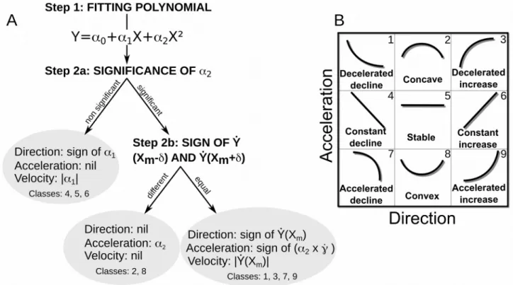
Figure 2: Classification steps (A) and classes (B). Once the second order polynomial Y = α0+α1X+α2X² is fitted (step 1), the significance of α2 is evaluated (step 2a) to distinguish between

linear (B. 4, 5 and 6) and non-linear (1, 2, 3, 7, 8 and 9) trajectories. For linear cases, assessing direction and velocity is straightforward using the coefficient of the slope α1. For non-linear

dynamics (step 2b), concave and convex cases (B. 2 and 8) can be discriminated by a change in the sign of the tangent around Xm. Remaining classes (1, 3, 7 and 9) require the calculation of the

curvature derivative at Xm as a proxy of the acceleration as well as the computation of the tangent

value at Xm for velocity estimation. B) Class numbering refers to the following types: accelerated

decline (1), concave (2), accelerated increase (3), constant decline (4), stable (5), constant increase(6), decelerated decline (7), convex (8), and decelerated increase (9).

Figure 3: Second order polynomial curves on the time interval [X0, XT], Xm being the middle of the

interval. For a given second order polynomial function Y = α0+α1X+α2X², six cases may be

described depending on the position of the curve relative to the interval [X0, XT]. For a convex

function (A), three cases can be found: a decelerated decline (A.1), a convex phase (A.2), or an accelerated increase (A.3). For a concave function (B), three cases as well can be identified: a decelerated increase (B.1), a concave phase (B.2) or an accelerated decline (B.3). The direction of the trajectory is assessed based on the sign of the tangents at points Xm-δ and Xm+δ (inset window).

Changing points are marked with a circle for p1 and a square for p2 and p3. p1 is the point where the

tangent becomes zero and delineated increase and decline. p2 and p3 are points where the tangent

Figure 4: Classification of the 108 bird species trajectories (standardised abundances) from 1989 to 2017 into the nine possible linear (D, E, F) and non-linear (A, B, C, G, H, I) classes. A) 1 accelerated declines, B) 4 convex trajectories, C) 0 accelerated increase, D) 24 constant declines, E) 33 stable trajectories, F) 23 constant increases, G) 4 decelerated declines, H) 16 concave trajectories, I) 3 decelerated increases. Scaled yearly indices of abundance (black dots) with sampling error (grey intervals) are shown for one species of each class. Second order polynomials are shown by a bold line and standard deviations by dashed lines. Changing points of interest are marked on these fits with their standard deviation (bounded segments) (circle and red for p1 and

Figure 5: Multi-species indicators (yearly values (black dots) with standard deviation (grey intervals)) of farmland (A) and forest (B) specialist species between 1989 and 2017. A) The second order polynomial is shown by a bold line and standard deviation by dashed lines. Changing point of interest is marked on this fit with its standard deviation (bounded segment) (square and blue for p3).

B) A stable fit is represented (bold line and standard deviation by dashed lines) as no linear trend