DOCTORAT DE L'UNIVERSITÉ DE TOULOUSE

(1)

DOCTORAT DE L'UNIVERSITÉ DE TOULOUSE

Délivré par :

Institut National Polytechnique de Toulouse (INP Toulouse) Discipline ou spécialité :

Dynamique des fluides

Présentée et soutenue par :

M. DAMIEN SZUBERT le lundi 29 juin 2015

Titre :

Unité de recherche : Ecole doctorale :

ANALYSE PHYSIQUE ET MODELISATION D'ECOULEMENTS TURBULENTS INSTATIONNAIRES AUTOUR D'OBSTACLES AERODYNAMIQUES A HAUT NOMBRE DE REYNOLDS PAR

SIMULATION NUMERIQUE

Mécanique, Energétique, Génie civil, Procédés (MEGeP) Institut de Mécanique des Fluides de Toulouse (I.M.F.T.)

Directeur(s) de Thèse : MME MARIANNA BRAZA

M. GILLES HARRAN Rapporteurs :

M. BRUNO KOOBUS, UNIVERSITE MONTPELLIER 2 M. GEORGE BARAKOS, UNIVERSITY OF LIVERPOOL

Membre(s) du jury :

1 M. ALAIN DERVIEUX, INRIA SOPHIA ANTIPOLIS, Président 2 M. FLAVIEN BILLARD, DASSAULT AVIATION, Membre 2 M. FRANK THIELE, TECHNISCHE UNIVERSITAT BERLIN, Membre

2 M. GILLES HARRAN, INP TOULOUSE, Membre

2 M. JEAN-PAUL DUSSAUGE, UNIVERSITE AIX-MARSEILLE 1, Membre

(2)

Acknowledgements

These three years and half spent in the Institut de Mécanique des Fluides de Toulouse let me time and opportunities to meet many people, researchers, colleagues, students, and friends I want to thank here.

I want above all to express my deepest thanks to my supervisor Marianna BRAZA, who oﬀered to me the opportunity to work in a practical way on ﬂuid dynamics, and more particularly on turbulence modelling in the context of the Com- putational Fluid Dynamics, involving various test cases described in this manuscript.

I was able to experience supervision of small groups of students, exchanging with them on technical and scientiﬁcal aspects. I also thank her a lot for helping me to survive in Stanford during summer 2014 after loosing my credit card, just before leaving France. Finally, I appreciated a lot the discussions we had concerning our vision of the World, society and humanity, with our respective experience and skills.

I am also very thankful to Prof. George Barakos for discussions we had regarding relations between research and industry, and for sharing is point of view regarding the situation of research more generally. I thank him as well as Flavien Billard, for their comments and corrections of this manuscript, as well as for sharing their special point of view on speciﬁc test cases.

I thank Prof. George Barakos and Prof. Bruno Koobus for having accepted the invitation to review my thesis. I also wish to thank all other members of the ex- amining committee: Alain Dervieux, Jean-Paul Dussauge, Gilles Harran and Prof.

Frank Thiele. I also thank Loïc Boudet, from DGA, and Prof. Julian Hunt, for taking part of the discussion during the defense. I would like to particularly thank Prof. Hunt for sharing his experience and his knowledge that conducted, among other, to the redaction of an article published in the Journal of Fluid Dynamics.

I want to express special thanks to Fernando Grossi, who helped a lot on physical and technical aspects when I arrived at IMFT for my internship and then for the beginning of my PhD while he was in ﬁrst year of his PhD, as well as during congresses. I appreciated a lot his point of view regarding the environment and method of work.

I would not have been able to do all the work presented here withtout the precious assistance of Yannick Hoarau, regarding mesh generation in particular, but also for technical, programming aspects, despite his huge amount of work, and I am very grateful for this. For this last point, I also want to thank Jan Vos, from

(5)

CFS Engineering, coordinator of the NSMB consortium, and who recieved me few days in his head quarters for implementing the transition model based on transport equations in NSMB.

My deepest gratitude to Parviz Moin, director of the Center for Turbulence Re- search, and his team, who received Marianna and me in Stanford during summer 2014, and Ik Jang, for the collaboration there. It was a great opportunity to discover a diﬀerent work environment as well as the culture and lifestyle in Stanford and in the Bay Area in general.

I thank again Gilles Harran, as well as Alain Sévrain, for their precious contribution to improve my expertise in signal processing as well as in ﬂuid-structure interactions.

My grateful thanks to Thibaut Deloze, Ioannis Asproulias, Wouter Van Veen, Antonio Jimenez Garcia, Saul Ferriera Perez, Vilas Shinde, Rogier Giepman and the BEI students for their precious contributions to the work presented in this manuscript. I also thank them, as well as Rémi Bourguet, Johannes Scheller, Math- ieu Marrant, Julie Albagnac, Simon Gsell and Christophe Korbuly for the enjoyable moments we had at the lab.

I thank all the services of the laboratory, from administration (Florence Colom- bies, Nadine Mandement, Aurélie Labrador, Denis Bourrel, Sandrine Chupin) to computing, reprography, documentation, as well as the direction of the lab, François Charru and Éric Climent, and of the group EMT2, Carlo Cossu, that allow researchers and students to work in a great environment in the IMFT and contribute to the cohesion of the research teams.

Finally, my relatives. First of all, Lucas, who oﬀered me opportunities to breath, to relieve, to open my mind, and to consider more and less seriously the future. I thank him for this and for his support during tough moments, during the ﬁnale rush in particular. I thank also Yann, with whom I shared more or less a similar journey, and for funny and cultural moments we had in Toulouse as well as for the discussions about the world in general. Thank you Amély, for being there for years, even if I moved quite far from you and you little family. I gratefully thank my parents, who really cared about my appetite and curiosity to explore and discover that crazy, incredible world, as well as my brother and sister.

A huge thank to Ciel mon doctorat. Any PhD student will understand.

The work presented in this memoir has been made possible thanks to the fel- lowship of the DGA (Direction Général de l’Armement) and the funding allocated by the ANR (Agence Nationale pour la Recherche) in the context of the Baresafe project (ANR-11-MONU-0004)

(6)

Nomenclature

Latin symbols

a Speed of sound

c Chord length

CD Drag coeﬃcient

CL Lift coeﬃcient

C_p Pressure coeﬃcient, C_p = (P −P∞)/(0.5ρ∞U∞²) dw Wall distance

D Cylinder diameter

f_{V K} Vortex-shedding frequency of the von Kármán instability

H Shape factor

k Turbulent kinetic energy l Turbulence length scale

L Distance between cylinders center

P Static pressure

Re Chord and diameter-based Reynolds number Reθ Momentum-thickness Reynolds number, ρθU∞/µ

Reθt Transition onset momentum-thickness Reynolds number Re_ν Vorticity Reynolds number, ρy²Ω/µ

St Strouhal number (St =fV KD/U∞)

t Physical time

t∗ Non-dimensionalised time (t∗=tU∞/c ort∗=tU∞/D) Tu Turbulence intensity, 100(2k/3)^1/2/U

U Local velocity

U^∞ Inlet reference velocity

x_t Laminar-turbulent transition location

(7)

Greek symbols

δ₉₉ Boundary-layer thickness δ^∗ Displacement thickness δij Kronecker delta

ε Turbulence dissipation rate γ Intermittency factor

γf, γair speciﬁc heat ratio of the ﬂuid and air λ_θ Pressure gradient parameter

µ Dynamic viscosity

ν Kinematic viscosity, µ/ρ ν_t Eddy viscosity

ω Speciﬁc turbulence dissipation rate Ω Absolute value of vorticity

ρ Fluid density

θ Momentum thickness

Abbreviations

ATAAC Advanced Turbulence Simulation

for Aerodynamic Application Challenges BSL Menter’s Baseline model

CFD Computational Fluid Dynamics DDES Delayed Detached-Eddy Simulation DNS Direct Numerical Simulation

MIV Movement induced vibration NSMB Navier-Stokes Multiblock

OSBLI Oblique-shock/boundary-layer interaction PIV Particle Image Velocimetry

POD Proper Orthogonal Decomposition PSD Power Spectral Density

RANS Reynolds-averaged Navier-Stokes

RMS Root mean square, RMS(x) = ^ñ1/N(x²₁+x²₂+. . .+x²_N) SA Spalart-Allmaras one-equation model

SST Shear Stress Transport model

SWBLI Shock-wave/boundary-layer interaction TFAST Transition Location Eﬀect

on Shock-Wave/Boundary-Layer Interaction TNT Turbulent/non-turbulent

TUD Technische Universiteit Delft or Delft University of Technology URANS Unsteady Reynolds-averaged Navier-Stokes

VIV Vortex induced vibration

WM-LES Wall-modelled Large Eddy Simulation

(8)

Mathematics

∇ Gradient, ∇U(x) =¹^∂U_∂x^x⁽^x⁾,^∂U_∂y^y⁽^x⁾,^∂U_∂z^z⁽^x⁾², with x= (x, y, z)

∇· Divergence, ∇ ·U(x) = div(U(x)) = ^∂U_∂x^x⁽^x⁾ +^∂U_∂y^y⁽^x⁾ + ^∂U_∂z^z⁽^x⁾

⊗ Tensor product

(9)

(10)

Chapter 1 Introduction

1.1 Objectives of this thesis

The present thesis investigates high-Reynolds number unsteady turbulent flows in- teracting with the solid wall from the low subsonic to the high-transonic and supersonic regimes, by means of numerical simulation. A specific attention is paid to the prediction of unsteady separation, including fluid-structure interaction aspects, as well as shock/boundary-layer and shock-vortex interaction. A considerable effort is devoted in the state of the fundamental research and applications domains in order to improve the simulation and turbulence modelling approaches (statistical (RANS, URANS), Large-Eddy Simulations (LES) and Hybrid (RANS-LES)) for the prediction of unsteady separation and reattachment, of natural instabilities and vortex structures responsible for movement induced vibration and acoustic noise around bodies, as well as prediction of shock-wave/boundary-layer interaction, a crucial issue for next generation of ‘laminar’ wing design with reduced drag and

(11)

CO2 emissions. A considerable effort is devoted internationally in order to provide more efficient High-Fidelity (Hi-Fi) approaches and to carry out modal analysis by suitable and specific methods, in order to elaborate reliable Reduced Order Mod- elling (ROM), which will allow for faster design cycles. The need of improvement of Hi-Fi and ROM approaches has been emphasized in a number of important interna- tional conferences as the 4^th and 5^th hybrid RANS-LES methods symposia (2012¹, 2014²), the ERCOFTAC symposium “Unsteady separation in Fluid-Structure interaction” 2013³, the biannual “Center for Turbulence Research” summer programme 2014⁴ and the “Whither Turbulence and Big Data” symposium 2015, among other.

Through these meetings clearly appears the continuous need of advancing in turbulence modelling eﬀorts in crucial regimes governed by strong adverse pressure gradients, by movement/deformation of the solid structure and by compressibility eﬀects in order to provide more improved predictions for the design.

This thesis aims at contributing in this context by studying turbulence modelling approaches and their ability to capture important phenomena and crucial instabilities arising in aerodynamics and hydrodynamics, as well as the unsteady loads evolution, crucial for the design and to develop a detailed physical analysis of the flow phenomena arising in the near-wall and near-wake regions. Further- more, it aims at providing a detailed modal analysis of the complex flow structure in order to prepare efficient reconstruction of the fields able to be used further on in ROM. These investigations have been carried out by means of well focused test-cases from the European Research programmes of the FP7: ATAAC⁵ (Advanced Turbu- lence simulations for Aerodynamic Application Challenges), coordinated by DLR - Göttingen, and TFAST⁶ (Transition location effect on shock wave boundary layer interaction), coordinated by IMP - Gdansk (Polish Academy of Science), as well as from the national ANR⁷ (Agence Nationale pour la Recherche) research programme Baresafe (Simulation of Safety Barrier Reliability), coordinated by EDF (Electricité de France).

1.2 Governing equations in fluid dynamics

In his Ph.D. thesis manuscript, Grossi (2014) described in a very comprehensive way the principles of the transport and governing equations in ﬂuid dynamics. This section re-uses his work.

Fluid motion is governed by three fundamental laws: conservation of mass, of momentum and of energy. These principles can be expressed through conservation laws, which describe the evolution of the conserved quantities in a given domain by means of transport equations. In the governing equations of fluid dynamics the flowfield is treated as a continuous medium. This means that the mean free path of the fluid molecules is assumed to be very small compared to the length scale charac-

1Fu et al. (2012),http://www.hrlm-4th.org

2Girimaji et al. (2014)

3http://www.smartwing.org/ercoftac

4https://ctr.stanford.edu

5http://cfd.mace.manchester.ac.uk/ATAAC/WebHome

6http://tfast.eu/

7http://www.agence-nationale-recherche.fr

(12)

1.2. Governing equations in fluid dynamics teristic of the problem (e.g. the diameter of a cylinder or the chord of an airfoil) so that the interaction between the fluid molecules is much more important than their individual motion. Therefore, the whole system can be investigated using continuum mechanics imagining a fluid particle a as very large number of fluid molecules within a small volume. All flow properties (as velocity, pressure, temperature, viscosity, etc.) are in fact mean properties which reflect the statistical motion of the fluid molecules at each point of the flowfield.

1.2.1 General transport equation

Assuming that φ is a scalar conserved quantity per unit volume and that V is an arbitrary control volume ﬁxed in space, the conservation law of φ states that the amount of this quantity insideV can vary as a result of its net ﬂux across the surface S enclosing V and due to volume and surface sources of φ only. This law can be formalized in integral form as:

∂

∂t

Ú

V φdV =−

Ú

S(FC·n)dS−

Ú

S(FD·n)dS+

Ú

V QVdV +

Ú

S(QS·n)dS. (1.1) The term on the left-hand side of Eq. 1.1 is the time variation of the total amount of φ inside V. The flux of φ across the volume boundaries is usually split into two components of different physical nature. FC is the ‘convective flux’, which corresponds to the time rate ofφ crossing the surfaceSper unit surface. Convective fluxes are directional, being proportional to and aligned with the local flow velocity U = [Ux, Uy, Uz]^T and are given by FC = φU. The second contribution, FD, is called ‘diffusive flux’ and is proportional and opposite to the gradient of φ. It is generalized by the ‘law of Fick’:

FD =−κρ∇

Aφ ρ

B

. (1.2)

whereκ is a diffusivity coefficient. The physical mechanism of diffusion is related to molecular agitation and can have a net effect even in a fluid at rest if the distribution ofφis inhomogeneous. The minus signs in front of the fluxes are due to the fact that the surface normal vector n is considered positive when pointing outwards (i.e. the dot products are negative when φ enters the control volume). QV and QS are the volume and surface sources, respectively. The resulting expression is a convection- diffusion equation in integral form, which allows the fluxes to be discontinuous (as in the case of shock-waves). Moreover, in the absence of volume forces, the variation of the conserved variable inside the control volume depends only on the net flux ofφ across the boundaries. A local differential form of the conservation law can be easily derived from the integral form. Using the divergence theorem (Gauss’ theorem), the surface integrals in Eq. 1.1 can be replaced by volume integrals of the divergences of the fluxes and surface sources. Also, assuming that the control volume is fixed in space, the time derivative on the left-hand side of the equation can be placed inside the integral (Reynolds’ transport theorem). Finally, since the integral form is written for an arbitrary control volume, the volume integrals can be dropped, yielding:

(13)

∂φ

∂t =−∇ ·FC− ∇ ·FD+QV +∇ ·QS, (1.3) which is valid at any point in the flowfield and requires the fluxes to be continuously differentiable (which is not always the case). It shows that surface sources are mathematically equivalent to fluxes and may be regarded in the same way. Moreover, if an equation is in conservative form, all the space derivative terms can be grouped as a divergence operator. Substituting the expressions obtained for the fluxes and rearranging the terms, one obtains:

∂φ

∂t =−∇ ·(φU) +∇ ·

C

κρ

Aφ ρ

BD

+QV +∇ ·QS. (1.4) In general, convective fluxes are non linear and yield first-order spatial derivatives while diffusive fluxes generate second-order ones. In the case where the conserved quantity is a vector, each component of φ can be regarded as a scalar quantity and the above equations can be applied. Alternatively, the equations written for a scalar property can be slightly modified, replacing the fluxes and surface sources by tensors and the volume source by a vector. Hence, the integral conservation equation for a vector reads:

∂

∂t

Ú

V φdV =−

Ú

S

1FC·n²dS−

Ú

S

1FD·n²dS+

Ú

V

QVdV +

Ú

S

1QS·n²dS. (1.5) where · stands for tensor. In diﬀerential form, Eq. 1.5 becomes:

∂φ

∂t =−∇ ·FC− ∇ ·FD+QV+QS. (1.6) Using tensorial notation (for the sake of simplicity), the convective and diﬀusive ﬂuxes are given by:

(FC)ij =φiUj, (FD)ij =−κρ ∂

∂xj

Aφi

ρ

B

. (1.7)

1.2.2 The Navier-Stokes equations

In this section, the three fundamental conservation laws that describe ﬂuid motion are derived, namely the continuity equation, the momentum equation and the energy equation. For viscous ﬂows, the resulting set of equations is commonly known as the ‘Navier-Stokes equations’.

1.2.2.1 Continuity equation

The principle of conservation of mass in a ﬂuid is expressed through the continuity equation, which states that mass cannot be created nor destroyed in the system.

The transported quantity is the fluid density ρ, which is a scalar quantity and has units of mass per unity volume. The continuity equation does not present a diffusive flux term since there is no mass diffusion in a fluid at rest. By replacing φ byρ in

(14)

1.2. Governing equations in fluid dynamics Eq. 1.1 and suppressing all source terms, the integral formulation of the continuity equation is obtained:

∂

∂t

Ú

V ρdV +

Ú

Sρ(U·n)ds= 0. (1.8)

The term in the left-hand side of Eq. 1.8 represents the time rate of change of mass inside a given control volume and the surface integral on the right side is the total mass flow across its boundaries. For the latter, negative values mean a net flux entering the control volume while positive ones correspond to an outflow. Applying Gauss’ and Reynolds’ theorems, the continuity equation written in differential form reads:

∂ρ

∂t +∇ ·(ρU) = 0. (1.9)

For incompressible ﬂows, ρ is constant and Eq. 1.9 reduces to ∇ ·U= 0.

1.2.2.2 Momentum equation

Newton’s second law states that the variation of the momentum of a body is equal to the net force acting on it. By applying this fundamental principle to a fluid, one obtains the momentum equation, which expresses the conservation of momentum in the fluid system. Since the momentum of a infinitesimally small fluid element of volumedV is defined asρUdV , the transported variable in the momentum equation is the momentum per unit volumeρU, which is a vector quantity. Alternatively, the conservation of momentum can be expressed by means of three separated transport equations for the individual components of momentum ρUx, ρUy and ρUz. As the continuity equation, the momentum equation has no diffusive flux since, by definition, the velocity (and thus the momentum) is zero in a fluid at rest. Hence, Eq. 1.5 applied for the transport of momentum yields:

∂

∂t

Ú

V ρUdV +

Ú

SρU(U·n)dS =

Ú

V

QVdV +

Ú

S

1QS·n²dS. (1.10) where the volume sources QV represent all existing body forces per unit volume, which act over dV and are also called external or volume forces (e.g. Coriolis, grav- itational, centrifugal and electromagnetic forces). The surface sources QS represent the second kind of forces that act on a ﬂuid element: the surface (or internal) forces.

In this group, there are the static pressure and the viscous stresses, which have a net eﬀect only on the boundary of the volume. The pressure P exerted by the surroundings acts in the direction normal to S, pointing inwards the ﬂuid element.

Therefore, the surface sources can be computed as −PI+σ, where I is the unit tensor and σ is the viscous stress tensor. In aerodynamics, the eﬀect of the gravi- tational force on the ﬂuid elements can be neglected and other volume sources are usually not present. Hence, the momentum equation becomes:

∂

∂t

Ú

V ρUdV +

Ú

SρU(U·n)dS =−

Ú

SP ¹I·n²dS+

Ú

S(σ·n)dS, (1.11) or in diﬀerential form:

(15)

∂ρU

∂t +∇ ·(ρU⊗U) =−∇P +∇ ·σ. (1.12) Since air behaves as a Newtonian ﬂuid, the shear stresses are proportional to the velocity gradients. Using tensorial notation, the general form of the viscous stress tensor σij reads:

σ_ij =µ

A∂Uj

∂xi

+∂Ui

∂xj

B

+λ∂Uk

∂xk

δ_ij, (1.13)

where the first index in the subscript indicates the direction normal to the plane on which the stress is acting while the second one gives its direction. If i = j the component is a ‘normal stress’ and otherwise, a ‘shear stress’. Shear stresses are generated by the friction resulting from the relative motion of a body immersed in a fluid or of different fluid layers. In Eq. 1.13, µ is the dynamic viscosity and λ is the second viscosity of the fluid. According to Stoke’s hypothesis for a Newtonian fluid in local thermodynamic equilibrium:

λ+ 2

3µ= 0. (1.14)

This relation is called ‘bulk viscosity’ and is a property of the fluid. It is responsible for the energy dissipation in a fluid of smooth temperature distribution submitted to expansion or compression at a finite rate. So far, there is no experimental evidence that Eq. 1.14 does not hold except for extremely high temperatures or pressures.

Using relation 1.14, Eq. 1.13 becomes:

σij =µ

A∂Uj

∂xi

+∂Ui

d ∂xj

B

− 2µ 3

∂Uk

∂xk

δij. (1.15)

Although the viscous stresses were derived as being surface sources, they play the role of diffusive fluxes of momentum (thus requiring fluid motion), with the dynamic viscosity acting as the diffusion coefficient.

1.2.2.3 Energy equation

In fluid dynamics, the conservation law for energy is obtained from the application of the first law of thermodynamics to a control volume. It expresses the fact that the time variation of the total energy inside a control volume is obtained from the balance between the work of the external forces acting on the volume and the net heat flux into it. In the energy equation, the transported quantity is the total energy per unit volume ρE, where E is the total energy per unit mass. It is defined as the sum of the internal energy per unit mass e (a state variable) and the kinetic energy per unit mass |U|²/2. The transport equation features a diffusive flux term which depends only on the gradient of e since, by definition, U = 0 at rest. It accounts for the effects of thermal conduction related to molecular agitation and is given by FD =−γfρκ∇e, where γf is the ratio of specific heat coefficients of the considered fluid, γf =cp/cv. For dry air at 20^◦C, γair = 1.4. Since the internal energy can be expressed in terms of the static temperature T by e = cvT, heat diffusion is more usually described using Fourrier’s law:

(16)

1.2. Governing equations in fluid dynamics

FD =−γfρκ∇e=−κ∇T, (1.16) where k is the thermal conductivity coeﬃcient (k = c_pρκ) and the negative sign accounts for the fact that heat is transferred from high- towards low-temperature regions.

Surface sources contribute to the energy equation through the work done by the pressure and viscous stresses (both normal and shear parts) acting on the boundaries of the ﬂuid element QS = −pU+ (σ·U). Therefore, neglecting the work done by body forces as well as that of internal energy sources (e.g. radiation, chemical reactions, etc.), the integral form of the energy equation reads:

∂

∂t

Ú

V ρEdV +

Ú

SρE(U·n)dS =−

Ú

SP(U·n)dS +

Ú

S(σ·U)·ndS+

Ú

Sk(∇T ·n)dS, (1.17) which is also frequently written in terms of the total enthalpy:

H =h+ |U|²

2 =E+P

ρ, (1.18)

where h is the enthalpy per unit mass. This yields:

∂

∂t

Ú

V ρEdV +

Ú

SρH(U·n)dS =

Ú

S(σ·U)·ndS+

Ú

Sk(∇T ·n)dS, (1.19) In diﬀerential form, Eq. 1.17 can be rewritten as:

∂ρE

∂t +∇ ·ρUE =−∇ ·PU+∇ ·(σ·U) +∇ ·(k∇T). (1.20)

1.2.2.4 Additional relations

In order to close the system of the Navier-Stokes equations, additional relations between the ﬂowﬁeld variables are needed. In aerodynamics, the air is usually modeled as a perfect gas and, therefore, a thermodynamic relation between the state variables P, ρ and T can be obtained by means of the equation of state:

P =ρRT, (1.21)

where R = cp −cv is the gas constant per unit mass (for a perfect gas, cp, cv and thus γf and R are constants). In compressible viscous flow, heating due to high velocity gradients is responsible for variations in the fluid viscosity. To account for such effect, a common practice in aerodynamics is to adopt Sutherland’s law (Sutherland, 1893), which expresses the dynamic viscosity µ of an ideal gas as a function of temperature only as:

µ µ_ref =

3 T T_ref

43/2 Tref +S

T +S . (1.22)

(17)

µref is a reference viscosity corresponding to the reference temperature Tref, and the constant S is the Sutherland’s parameter (or Sutherland’s temperature). Values commonly used for air areµref = 1.715×10⁻⁵Pa.s,Tref = 273.15K andS = 110.4K.

Sutherland’s Law gives reasonably good results at transonic and supersonic speeds.

For hypersonic ﬂows, however, more elaborated formulas are usually employed.

The thermal conductivity coeﬃcient k varies with temperature in a similar way to µ. For this reason, the Reynolds’ analogy is frequently used to computek, reading:

k =cp

µ

Pr (1.23)

where Pr if the Prandtl number, which is usually taken as 0.72 for air.

1.2.3 The Reynolds-averaged Navier-Stokes equations

According to ‘Morkovin’s hypothesis’, the effect of density fluctuations on turbulent eddies in wall-bounded flows is insignificant provided that they remain small compared to the mean density. Indeed, this hypothesis is verified up to Mach numbers of about five (Blazek, 2005) and, therefore, a common approach in turbulence modeling is to apply ‘Reynolds averaging’ to the flow variables (otherwise one should use Favre averaging).

In Reynolds averaging, the flow variables are decomposed into two parts: a mean part and a fluctuating part. The velocity, for instance, is represented as U =U+U^′, whereU is its mean value andU^′its instantaneous fluctuation. For stationary turbulent flows,U is normally computed using time-averaging, which is the most common Reynolds-averaging procedure and is appropriate for a large number of engineering problems. Time-averaging can also be used for problems involving very slow mean flow oscillations that are not turbulent in nature, as long as the characteristic time scale of such oscillations is much larger than that of turbulence. In this way, the mean velocity is computed as:

U = lim

T→∞

Ú t+T

t U dt (1.24)

Also, by definition, the average of U^′ i is zero. Substituting the flow variables in the Navier-Stokes equations by Reynolds-averaged ones and taking the average, obtains in differential form:

∂ρ

∂t + ∂

∂xi

(ρUi) = 0, (1.25)

∂

∂t(ρUi) + ∂

∂xj

(ρU¯iU¯j) =−∂P

∂xi

+ ∂

∂xj

(σij +τij), (1.26)

∂

∂t

1ρE²+ ∂

∂xj

1ρU¯jE²=− ∂

∂xj

1P¯U¯j

2+ ∂

∂xj

[(σij +τij)] + ∂

∂xj

A

k∂T

∂xj

+qtj

B

. (1.27) The only diﬀerence between the Reynolds-averaged Navier-Stokes (RANS) equations shown above and the original set of Navier-Stokes equations is the existence of a turbulent stress tensor τij = −ρU¯ _i^′U_j^′ (also called Reynolds stress tensor) and

(18)

1.2. Governing equations in fluid dynamics of a turbulent transport of heat qtj. Both quantities are computed by means of additional equations (the so-called ‘turbulence models’) whose equations are reported in appendix A page 135.

1.2.4 The eddy-viscosity assumption

In the previous subsection, the Reynolds-averaged Navier-Stokes equations were presented and the turbulent stress tensor τij and the turbulent heat ﬂux qij were introduced. In this thesis, all turbulence models make use of Boussinesq hypothesis (Boussinesq, 1877), which relates the turbulent stresses to the mean-ﬂow velocity gradients by:

τij = 2µtSij − 2

3ρkδij, (1.28)

where µt is a scalar ‘eddy viscosity’ (also called turbulent viscosity) and Sij is the mean strain-rate tensor.

The Boussinesq hypothesis assumes that the principal axes of the turbulent stress and mean strain-rate tensors are collinear and is unable to capture anisotropy eﬀects of the normal turbulent stresses. In practice, however, Eq. 1.28 provides accurate results for many engineering applications, including aerodynamic ﬂows.

Based on the concept of eddy viscosity, the turbulent heat ﬂux is then calculated by means of the ‘Reynolds analogy’:

q_t_j =−k_t∂T

∂xj

=−c_p µt

Prt

∂T

∂xj

, (1.29)

where kt is the turbulent thermal conductivity coeﬃcient and Prt is the turbulent Prandtl number (which for air is 0.9).

1.2.5 Organised-Eddy Simulation

Details of the Organised-Eddy Simulation (OES) method used in the 3D conﬁgu- ration of a tandem cylinders (chapter 2 page 13) as well as in the 2D simulation of a supercritical airfoil (chapter 3 page 51) have been published in Bourguet et al.

(2008). This method was described as follows: The statistical turbulence modelling offers robustness of the simulations in this region at high Reynolds numbers but it has proven a strong dissipative character that tends to damp crucial instabilities oc- curring in turbulent flows around bodies, as for example low frequency modes as von Kármán instability, buffet or flutter phenomenon. The OES (Organised-Eddy Sim- ulation) approach offers an alternative that is robust and captures the above physical phenomena. This approach consists in splitting the energy spectrum in a first part that regroups the organised flow structures (resolved part) and a second part that includes the chaotic processes due to the random turbulence (to be modelled).

In the time-domain, the spectrum splitting leads to phase--averaged Navier-Stokes equations (Jin and Braza, 1994). A schematic illustration of the OES approach is presented in Fig.1.1. The turbulence spectrum to be modelled is extended from low to high wavenumber range and statistical turbulence modelling considerations can be adopted inducing robustness properties. However, the use of standard URANS modelling is not suﬃcient in this case. In non-equilibrium turbulence, the inequality

(19)

Figure 1.1: Sketch of the energy spectrum splitting in OES: (a) energy spectrum, (b) coherent part (resolved) and (c) random, chaotic part (modelled). kc denotes coherent process wavenumber.

between turbulence production and dissipation rate modiﬁes drastically the shape and slope of the turbulence spectrum in the inertial range (Fig. 1.1), comparing to the equilibrium turbulence, according to Kolmogorov’s cascade (slope equals to

−5/3). This modification has been quantified by the experimental study of Braza et al. (2006). Therefore, the turbulence scales used in standard URANS modelling have to be reconsidered in OES, to capture the effects due to the non-linear interaction between the coherent structures and the random turbulence. In the context of the OES approach, a modification of the turbulence scales in two-equation models was achieved on the basis of the second-order moment closure (Bourdet et al., 2007).

By using the Boussinesq law 1.28 as well as the dissipation rate and the turbulent stresses evaluated by DRSM, a reconsidered eddy-diﬀusivity coeﬃcient was derived.

It was shown that the Cµ values were lower (order of 0.02) than the equilibrium turbulence value (Cµ = 0.09) in two-equation modelling. Furthermore, the turbulence damping near the wall needed also to be revisited because of the diﬀerent energy distribution between coherent and random processes in non-equilibrium near-wall regions. A damping law with a less abrupt gradient than in equilibrium turbulence was suggested, f_µ= 1−exp(−0.0002y⁺−0.000064y⁺²)(Jin and Braza, 1994).

The eﬃciency of the OES approach in 2D and 3D has been proven in a number of strongly detached high Reynolds number ﬂows, especially around wings (Hoarau et al., 2006), as well as in the context of DES (El Akoury, 2007).

1.3 Thesis outline

This Ph.D. was a great opportunity to work on three main test-cases, covering a wide range of Mach numbers at high Reynolds numbers, by means of advanced statistical CFD methods.

The ﬁrst conﬁguration is a tandem of two inline cylinders at Mach number 0.12.

The main flow features in static as well as in dynamic case, with the downstream cylinder free to move crosswise, is studied at this subsonic velocity. The results are given in chapter 2 (page 13). The transonic flow around two different supercritical airfoils, in the Mach number range 0.70–0.75, is next studied. Detailed results of the study around the OAT15A airfoil, involving time-frequency as well as POD analysis, and introducing a stochastic forcing method focussing on the Turbulent/- non-Turbulent interfaces prediction, are presented in chapter3(page51) by means of

(20)

1.3. Thesis outline an article published in the Journal of Fluids and Structures (Szubert et al., 2015b) in included in this manuscript. The V2C proﬁl has also been studied in the context of the TFAST european project in 2D and 3D, involving laminar/turbulent transition location study, and the results have been detailed in an article submitted to the European Journal of Mechanics – B\Fluids, and also included in this manuscript (section 3.2 page 81. Finally, the predictive capabilities of a hybrid RANS-LES model, on the one hand, and of a wall-modelled LES, on the other hand, have been analysed during the summer programme 2014 handled by the Center for Turbulence Research, CA. All the results of this study are presented in chapter 4 (page 117) by means of the proceeding following the programme. The last chapter (page 129) is the conclusion of this manuscript. Appendices have also be written for extra contributions, such as a page/poster containing the equations of the γ−Reθ two- equation transition model for implementation consideration, as this work as been done during this Ph.D., or a short user guide of the post-processing software Tecplot, for future users to beneﬁt my knowledge of this complex but powerful software.

(21)

(22)

Chapter 2 Tandem of two inline cylinders

2.1 Flow analysis - Static case . . . . 14 2.1.1 Context . . . 14 2.1.2 Test-case description . . . 15 2.1.3 Numerical method . . . 16 2.1.4 Results . . . 18 2.1.4.1 Flow overview . . . 18 2.1.4.2 Convergence study. . . 20 2.1.4.3 Turbulence model study . . . 21 2.1.4.4 POD analysis. . . 27 2.1.5 3D Simulations . . . 41 2.2 Fluid-structure interaction - Dynamic case . . . . 43 2.2.1 Introduction . . . 43 2.2.2 Results . . . 43 2.2.2.1 Fluid-structure interaction . . . 43 2.2.2.2 POD analysis. . . 45 2.3 Conclusion . . . . 49

The tandem cylinder arrangement is a canonical problem to advance modeling techniques for flow interactions. Tandem cylinders with similar diameters can be found in several locations on a landing gear, such as multiple wheels, axles, and hydraulic lines. This configuration can be found in cooling, venting systems, or platform support. In section 2.1, the modelling capabilities as well as the physics around two static inline cylinders are studied. In section 2.2, the fluid-structure problems are considered by giving one degree of freedom in translation to the downstream cylinder.

(23)

2.1 Flow analysis - Static case

2.1.1 Context

The 36-month ATAAC (Advanced Turbulence Simulation for Aerodynamic Applica- tion Challenges) European project, ended in 2012, handled sereval geometries with the aim of investigating the capabilities of turbulence modelling approaches available in CFD methods to model complex aerodynamic flows at high Reynolds number. 21 partners focussed on restricted set of CFD approaches: Differential Reynolds Stress Models (DRSMs), advanced Unsteady RANS models, Scale-Adaptive Simulation (SAS), Wall Modelled LES and different hybrid RANS-LES coupling schemes. Ba- sic URANS models show indeed their limits in the case of complex situations such as stall, detached flows, high-lift applications, swirling flows, buffet, etc.

Figure 2.1: Main landing gear of a Cessna 404 Titan.

The tandem of two inline cylinders have been selected as one of the test cases handled for this project. The averaged and unsteady characteristics of the ﬂow, in the ﬂow and at the surface of the two cylinders, had previously been studied in a series of experiments performed in NASA Langley Research Center leading to a detailed set of data.

This configuration is a model for interaction problems commonly encountered in airframe noise configurations (e.g. hydraulic lines, support and hoses on a landing gear, Fig. 2.1). It involves many complex flow phenomena: separation of turbulent boundary layer and free shear layer roll-up, interaction of unsteady wake of the front cylinder with the downstream one, unsteady massively separated flow in the wake of the rear cylinder, etc. In this context, in a “noise-prediction” orientation of the numerical study in particular, conventional unsteady RANS approaches are not applicable and the capa- bility of the aforementioned numerical methods to

accurately reproduce the ﬂow and predict noise have been investigated during the ATAAC project.

The ﬂow around a single cylinder and the wake past of it have been well in- vastigated at moderate and high Reynolds numbers, experimentally (e.g. Roshko, 1954;Williamson, 1992;Perrin et al., 2007) and numerically (e.g.Braza et al., 1986;

Persillon and Braza, 1998; Braza et al., 2001), identifying several flow regimes as a function of the Reynolds number. The flow is laminar up to Re ≈ 200, with two symmetrical recirculation vortices just downstream the cylinder. From Re ≈ 40, the symmetry is broken due to the stream pertubations and the counter rotating vortices are alternatively detached and convected in the flow. This two-dimensional phenomenon generates a series of vortices called the von Kármán street. The vortices are detached periodically and the corresponding frequency of the detachment

(24)

2.1. Flow analysis - Static case

is non dimensionalised to give the Strouhal number:

St = fV KD U∞

(2.1) where fV K is the frequency of the vortices detachment (two successive detachments of the counter-rotating vortices is one period of the phenomenon), D the diameter of the cylinder (or the characteristic length of the body) and U∞ the freestream velocity of the flow. The Strouhal number depends on the body shape and the Reynolds number. This periodical detachment is caracterised by a time evolution of the aerodynamic forces applying on the body atf_{V K} for the perpendicular ones (lift) and fV K/2 for the streamwise ones (drag). Close to Re ≈ 200, three-dimensional effects can be observed: the von Kármán vortices ondulate in the crosswise direction, parallel to the cylinder, with a wavelength of about 4D. For Reynolds numbers higher than 200, this wavelength is reduced to 1D and first turbulence phenomena develop in the wake. The flow is fully turbulent for Re> 300 which is the case in this study, as the Reynolds number equals to 166,000 as detailed in the next section.

A first synthesis of numerical simulations carried out for this test case was carried out by Lockhard, regrouping 13 contributions involving different modelling approaches, as well as previous simulations by Khorrami et al. (2007), using URANS SST. These simulations indicated that the majority of the approaches captured quite well the Strouhal number of the vortex shedding frequency around the first cylinder, (St = 0.24). Furthermore, as is seen in the ATAAC European program, the DES approaches better capture the complex vortex dynamics of the present flow, especially the formation of Kelvin-Helmholtz vortices in the separated shear layers. In the experimental context, it was found that the shear layers formed downstream of the first cylinder wrap around the second cylinder and interact non-linearly with the complex turbulence background, producing predominant frequencies in the energy spectrum, in the range of acoustic noise. Moreover, the numerical studies reported by Lockard in the context of the workshop for airframe noise computation, evaluated the mean drag coefficient provided by the different simulations, that had shown quite a dispersion among the different studies, with a most probable mean value of order 0.484 around the first cylinder.

2.1.2 Test-case description

Figure 2.2: Experi- mental set-up.

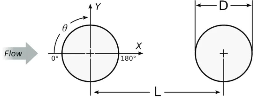
Three series of experiments have been carried out on this geometry. The first set was conducted in the subsonic, at- mospheric NASA-Langley Basic Aerodynamics Research Tunnel (BART; Fig. 2.2), and aimed at analysing the overall flow properties around the cylinders, by means of Particle Image Velocimetry (PIV) and hot-wire measurements (phase 1 of BART experiments, Jenkins et al., 2005). The second set of experiments was conducted in the same wind tunnel and aimed at measuring detailed average and unsteady pressure distribution at the surface of the cylinder, using static pressure orifices and piezore- sistive, differential pressure transducers on the two cylin-

(25)

L

!

0° 180°

Y

X

D

Flow

Figure 2.3: Diagram of the cylinders tandem and coordinate reference system.

ders (phase 2, Jenkins et al., 2006). The cylinders diameter has been slightly increased for this study to accommodate the pressure tubing and electrical wiring, but flow velocity has been adapted to keep the same Reynolds number, 1.66×10⁵. The freestream turbulence level measured in this wind tunnel was less than 0.10%. Fi- nally, the acoustic environment of this configuration have been studied in the Quiet Flow Facility (QFF) at NASA Langley (Lockard et al., 2007). While the QFF is an open jet facility specifically designed for anechoic testing, the flow has been adapted to obtain the same shedding frequency as in the BART experiments. All the facility dimensions and the flow properties are summarised in Table 2.1, in the next section presenting the numerical method. To ensure a fully turbulent shedding process, the boundary layers on the upstream cylinder were tripped between azimuthal locations of 50 and 60 degrees and −50and −60 degrees

2.1.3 Numerical method

This study has been carried out by using the Navier-Stokes Multiblock (NSMB) solver. The main properties of this code have been presented in Szubert et al.

(2015b), among other articles. This article details a major part of the work achieved during this Ph.D. study and has been included in this manuscript in subsection3.1.1 of chapter 3, page 52. The reader is invited to read the section of this article dedicated to the NSMB code.

In the context of the ATAAC programme, the numerical study has been performed with non-dimensional parameters. The velocity, the density, the temperature and the cylinders diameter have been set to the unity. This leads to the value of 43.2579 for the static pressure P and the gas constant:

P =ρRT, a=^ñγairRT , M = U

a (2.2)

Finally:

P =R = 1 M²γair

(2.3) The time has also been non-dimentionalised as follows: t^∗ =tU∞/D.

The main numerical and experimental parameters can be compared in Table2.1.

H/D is the non-dimensionalised height or span of the cylinders, and W/D is the non-dimensionalised width of the wind tunnel in the test section.

(26)

BART QFF CFD

Phase 1 Phase 2

D 0.04445 m 0.05715 m 0.05715 m 1

L/D 3.7

H/D 16.0 12.4 16.0 3

W/D 22.9 17.8 10.7 17.8

Mach 0.1635 0.1285 0.1274 0.1285

U^∞ 56.0 m.s^-1 44.0 m.s^-1 43.4 m.s^-1 1

Re 1.66×10⁵

Table 2.1: Experimental and numerical main parameters of the tandem cylinders geometry and ﬂow

The 4^th order skewsymmetric central scheme has been used for the space dis- cretisation. Implicit time integration using the dual time stepping technique with 3 Gauss-Seidel iterations has been performed. Since NSMB solves the compressible Navier-Stokes and models equations, the preconditioning ofWeiss and Smith (1995) is used to solve the flow at the Mach number 0.1285. This choice has been validated by Marcel (2011) for a Mach 0.18 flow through a confined bundle of cylinders by using the same CFD code.

The grid has been provided by the NTS (New Technologies and Services) partner from Saint Petersburg, Russia, in the context of the ATAAC programme. The grid is divided in 16 blocks of the parallel computation, and have approximately 156,000 volume cells. The gridlines are shown in Fig. 2.4 for the whole domain and around the two cylinders. The grid is slightly reﬁned around the downstream cylinder has more turbulence is expected. The non-dimentionnalized ﬁrst-cell height around this cylinder is 3.4×10⁻⁵ while it is5×10⁻⁵ for the upstream one. The total length of the domain is 44D.

On the solid wall, impermeability and no-slip conditions are employed. The far- ﬁeld conditions are characteristic variables with extrapolation in time. The upstream turbulence intensity is set to TU = 0.08%.

(27)

Figure 2.4: Multiblock domain of the tandem of cylinders.

2.1.4 Results

2.1.4.1 Flow overview

Eight snapshots of the vorticity field from a preliminaryk-ω-SST simulation covering one period of the von Kármán phenomenon can be observed in Fig. 2.5. The main characteristic of the field is that the vortex shedding occurs at the same frequency for the two cylinders, due to the wake of the first cylinder that intensively influences the generation of vortices by the second cylinder. The distance L/D= 3.7between the two cylinder is optimal to observe this phenomenon. In case of a smaller or a bigger distance, the vortex shedding would be in phase opposition between the two cylinders, generating a more complexe wake downstream the whole geometry.

After this preliminary overview of the ﬂow structure, a numerical study is carried out in order to determine the best convergence criterion and turbulence models to simulate this test case. These parameters don’t change the overall ﬂow structure and the above description remains valid.

(28)

Figure 2.5: Snapshots of the vorticity ﬁeld by k-ω-SST simulation covering one period of von Kármán.

(29)

2.1.4.2 Convergence study

In the context of the dual-time stepping, a sensitivity study of the physical results regarding the tolerance of the convergence criterion is ﬁrst carried out. The convergence criterion at the inner step n is deﬁned by the ratio between the L₂−norm of the density equation residual at the inner step n and the one at the initial inner step. It is calculated at each inner computation step and when the tolerance is reached, the physical solution is saved at the current physical time step and the process goes on at the next outerstep. The system of equations needs to converge enough to provide a good prediction of the physical solution. However, a very low tolerance implies long computation time to reach the requested value and becomes useless compared to the numerical uncertainties (time and grid resolutions, com- puter precision). This study is performed to determine the better tolerence for the three-dimensional computations.

For this study, the k-ω-SST model of Menter (1994) (see also section A.2.3.2 of appendix A, page 141) is used, as it is well designed for ﬂows under high pressure gradient, and the non-dimensionalised time step ∆t^∗ = 0.00845 has been chosen from the ATAAC programme.

The RMS value of the lift and drag coefficient fluctuations of the two cylinders are calculated at each outerstep. The last steps are plotted in Fig.2.6 for the three tolerance values analysed. The curves trend shows at first glance that the difference between the two smaller tolerances is less than between 10⁻³ and 10⁻⁴. While the physical solutions were well converged, small oscillations are visible in the RMS values and are due to numerical resolution.

Figure 2.6: Evolution of the RMS values of the lift and drag coeﬃcients ﬂuctuations for three convergence tolerances.

The ﬁnal values of the RMS, as well as the mean of the lift and drag coeﬃcients, are reported in Table 2.2 for a quantitative comparison. The three tolerances give

(30)

Tol. Upstream cylinder Downstream cylinder

C_D C_L RMS(C_L^′) RMS(C_D^′ ) C_D C_L RMS(C_L^′) RMS(C_D^′ ) 10⁻³ 0.7997 0.0022 0.0512 0.5765 0.2035 -0.0020 0.2590 1.1363 10⁻⁴ 0.7990 0.0028 0.0509 0.5746 0.2047 -0.0036 0.2584 1.1370 10⁻⁵ 0.7991 0.0027 0.0510 0.5749 0.2045 -0.0049 0.2583 1.1377

Table 2.2: Mean values of the lift and drag coeﬃcients and RMS values of their ﬂuctuactions for the two cylinders.

very close results with a diﬀerence < 1%, except for the mean lift value on both cylinders. Between 10⁻³ and 10⁻⁴, CL is increased by 20% on the ﬁrst cylinder and 44% on the second one, while between 10⁻⁴ and 10⁻⁵, CL is 4% smaller on the upstream cylinder, and 27% higher on the downstream one. In the spirit of getting meaningful physical results in a reasonnable computation time, the tolerance 10⁻⁴ is retained for the the remaining simulations.

2.1.4.3 Turbulence model study

A similar comparison is carried out to compare the results of four turbulence models.

The mean and RMS values of the lift and drag coeﬃcient time evolution are reported in Table 2.3. The Edwards and Chandra (1996) modiﬁed Spalart and Allmaras (1994) (see also section A.1.1 of appendix A, page 135) and the k-ω-SST (Menter, 1994 and section A.2.3.2 page 141) give very close results in mean and amplitude.

The k-ω-BSL (Menter, 1994 and section A.2.3.1 page 139) is more dissipative and as a consequence, the amplitude of the aerodynamic coeﬃcients are smaller.

Models Upstream cylinder Downstream cylinder

CD CL RMS(C_L^′) RMS(C_D^′ ) CD CL RMS(C_L^′) RMS(C_D^′ ) SA-E 0.7826 0.0028 0.0742 0.6246 0.2008 0.0018 0.3068 1.3295 k-ω-SST 0.7990 0.0028 0.0509 0.5746 0.2047 -0.0036 0.2581 1.1370 k-ω-BSL 0.5567 0.0011 0.0167 0.2523 0.2852 -0.0054 0.1246 0.8045

Table 2.3: Mean values of the lift and drag coeﬃcients and RMS values of their ﬂuctuactions for three turbulence models.

The mean streamlines in the wake of each cylinder are plotted for the three turbulence models in Fig. 2.7. The overall prediction of the flow is similar between the three models and the experiment (Fig. 2.8) and the symmetry between the upper and lower sides of the flow is observed. However, they predict slight different size of the recirculation area, in particular none of them matches the experimental measurements.

The non-dimensionalised streamwise velocity at y = 0 measured in the wake of the two cylinders is plotted in Fig. 2.9, and the recirculation lengths (x∧U(x) = 0) are reported in Table 2.4. In the BART experiment, the second recirculation has been reduced by 80% compared to the ﬁrst. This diﬀerence might by due to the position of the cylinders compared to each other. The velocity in the wake of the

(31)

(A) (B) (C)

Figure 2.7: Comparison of the mean streamlines in the wake of the upstream (top) and the downstream (bottom) cylinders. (A) SA-E, (B) k-ω-SST, (C) k-ω-BSL.

(A) (B)

Figure 2.8: Mean stream lines from PIV measurments. (A) Upstream cylinder, (B) Downstream cylinder (Jenkins et al., 2005).

(32)

(A) (B)

Figure 2.9: Comparison between turbulence models en experiment of normalised streamwise velocity in the wake. (A) Upstream cylinder, (B) Downstream cylinder.

ﬁrst cylinder is limited by the presence of the second cylinder and this favours the development of the vortices before they detach, while this is not the case for the second cylinder. However, this phenomenon is not observed in the simulations, which give an opposite trend, and the diﬀerence between the two regions is less important (SA-E and k-ω-SST: +20%,k-ω-SST: +67%).

Models/Source L_recirc/D

Upstream cyl. Downstream cyl.

PIV (Jenkins et al., 2005) 1.2 0.25

SA-E 0.4 0.5

k-ω-SST 0.45 0.75

k-ω-BSL 0.75 0.9

Table 2.4: Recirculation length downstream each cylinder.

Spectral analysis

A spectral analysis is carried out on the time evolution of the lift and drag coeﬃcients recorded at a physical time step∆t^∗ = 0.00845, the same as the simulation itself. All signals are 17751 sample length, and are processed by the Welch’s method (Welch, 1967) with the following parameters:

• Window: Hanning,

• Window size: Nwind= 8192 samples,

• Overlap: 65%,