Why Is Europe More Equal Than the United States?

HAL Id: halshs-03022133

https://halshs.archives-ouvertes.fr/halshs-03022133

Preprint submitted on 24 Nov 2020

HAL is a multi-disciplinary open access

archive for the deposit and dissemination of sci-entific research documents, whether they are pub-lished or not. The documents may come from teaching and research institutions in France or

L’archive ouverte pluridisciplinaire HAL, est destinée au dépôt et à la diffusion de documents scientifiques de niveau recherche, publiés ou non, émanant des établissements d’enseignement et de recherche français ou étrangers, des laboratoires

Why Is Europe More Equal Than the United States?

Thomas Blanchet, Lucas Chancel, Amory Gethin

To cite this version:

Thomas Blanchet, Lucas Chancel, Amory Gethin. Why Is Europe More Equal Than the United States?. 2020. �halshs-03022133�

Why Is Europe More Equal Than the United States?

Thomas Blanchet

Lucas Chancel

Amory Gethin

September 2020

WHY IS EUROPE MORE EQUAL

THAN THE UNITED STATES?

⇤

T

B

L

C

A

G

Abstract

We combine all available household surveys, income tax and national accounts data in a systematic manner to produce comparable pretax and posttax income inequality series in 38 European countries between 1980 and 2017. Our estimates are consistent with macroeconomic growth rates and comparable with US Distributional National Accounts. We find that inequalities rose in most European countries since 1980 both before and after taxes, but much less than in the US. Between 1980 and 2017, the European top 1% pretax income

⇤_{Thomas Blanchet, Paris School of Economics – EHESS, World Inequality Lab:}

thomas.blanchet@wid.world; Lucas Chancel, World Inequality Lab, Paris School of

Eco-nomics and IDDRI, SciencesPolucas.chancel@psemail.eu; Amory Gethin, World Inequal-ity Lab – Paris School of Economics: amory.gethin@psemail.eu. This is a revised and extended version of the work by the same authors that previously circulated under the title “How Unequal is Europe? Evidence from Distributional National Accounts, 1980-2017”. We thank Daron Acemoglu, Facundo Alvaredo, Andrea Brandolini, Bertrand Garbinti, Jonathan Goupille-Lebret, Antoine Bozio, Stefano Filauro, Ignacio Flores, Branko Milanovic, Thomas Piketty, Dani Rodrik, Emmanuel Saez, Wiemer Salverda, Daniel Waldenstr¨om, and Gabriel Zucman for helpful comments on this paper. We are also grateful to Alari Paulus for his help in collecting Estonian tax data. Mat´eo Moisan provided useful research assistance. We acknowledge financial support from the Ford Foundation, the Sloan Foundation, the United Nations Development Programme, the European Research Council (ERC Grant 856455), and the Agence Nationale de la Recherche (EUR Grant ANR-17-EURE-0001).

share rose from 8% to 11% while it rose from 11% to 21% in the US. Europe’s lower inequality levels are mainly explained by a more equal distribution of pretax incomes rather than by more equalizing taxes and transfers systems. “Predistribution” is found to play a much larger role in explaining Europe’s

relative resistance to inequality than “redistribution”: it accounts for between two-thirds and ninety percent of the current inequality gap between the two regions.

JEL codes: H23, H24, H51, H52, H53, E01.

I. INTRODUCTION

While inequality has attracted a considerable amount of attention in recent aca-demic and policy debates, basic questions about the distribution of growth and redistribution remain unanswered. To what extent was the remarkable rise in income inequality in the US over the past decades inevitable? What can be learned from the study of inequality and growth in other high income countries, and in particular European nations, to answer this question? The comparative study of the distribu-tion of growth, taxes and transfers can provide critical insights into such debates. However, to date, inequality and redistribution estimates across countries have been hard to interpret because of a lack of conceptual and empirical consistency.

The standard source to measure economic growth across countries is the national accounts, while the standard source to measure and analyse inequality and redistri-bution across countries is household surveys. Surveys are known to underrepresent top incomes and do not add up to macroeconomic income totals, leading to poten-tial inconsistencies in the study of growth, inequality and redistribution. In order to address some of these limitations,Piketty and Saez (2003),Piketty (2003)and several authors have relied on tax data to study long run trends in inequality. Yet tax data also has a lot of issues in terms of comparability and consistency. In particular, tax data measures concepts that vary between countries, and miss the large share of income that goes untaxed. To overcome this problem,Alvaredo et al. (2016)and

Piketty, Saez, and Zucman (2018)developed “Distributional National Accounts”

income, and established guidelines to carry out this work in other parts of the world. This work has attracted interest from academics (triggering important method-ological debates1_{) and policymakers but unfortunately, with the exception of France}

(Bozio et al., 2018;Garbinti, Goupille-Lebret, and Piketty, 2018) similar work in

comparable countries remains rare. This makes it difficult to compare the situation of the United States with other countries. In Europe, the lack of estimates of the income distribution that integrate surveys, tax and national accounts are not the result of a lack of data per se. In fact, there is a fair amount of data available, at least since the 1980s. The problem is that these data are scattered across a variety of sources, taking several forms, using diverse concepts and different methodologies. So we find ourselves with a disparate set of indicators that are not always comparable, are hard to aggregate, provide uneven coverage, and can tell conflicting stories.

As a result, the literature has so far struggled to answer basic questions, such as whether European inequality as a whole is similar to that of the US, whether this has changed over time, and whether the differences between Europe and the US are due to pretax inequality or to redistribution. This paper addresses these substantive and methodological issues by constructing the first distributional national accounts for 38 European countries since 1980, which are comparable with recently produced dis-tributional national accounts for the US. While we still face considerable challenges in the construction of good estimates of the income distribution in some countries, we believe that the series described in this paper present major improvements over existing ones.

Our estimates combine virtually all the existing data on the income distribution of European countries in a consistent way. That includes, first and foremost, household surveys, national accounts, and tax data. It also includes additional databases on social contribution schedules, social benefits by function, and government spending on health that have been compiled by several institutions over the years (OECD, Eurostat, WHO). Our methodology exploits the strengths of each data source to correct for the weaknesses of the others. It avoids the kind of systematic errors that would arise from the comparison of different income concepts, different statistical units and different methodologies. As such, our estimates are meant to reflect the

best of the literature’s knowledge on what has been the evolution of inequality in Europe.

In line with the logic of Distributional National Accounts (DINA), we distribute the entirety of the national income. This includes money that never explicitly shows up on anyone’s bank account, such as imputed rents, production taxes or the retained earnings of corporations, yet can account for a significant share of the income recorded in national accounts and official publications of macroeconomic growth. Therefore, our results are consistent with macroeconomic totals, and provide a comprehensive picture of how income accrues to individuals, both before and after government redistribution. Using a broad definition of income makes our results less sensitive to various legislative changes, and therefore more comparable both over time and between countries.

Rather than focusing on a handful of indicators, we cover the entire distribution from the poorest income groups (well covered by household surveys) to the top 0.001% (which we can capture thanks to tax data) for income both before and after redistribution. We can aggregate our distributions at different regional levels, and analyze the structure of inequality with a good level of detail. We can use our estimates to compute any set of synthetic indicators (such as top and bottom income shares, poverty rates or Gini coefficients) in a consistent way at the country or regional level. We can test how all these results are affected by alternative assumptions on the distribution of unreported income or on the mismeasurement of top incomes in surveys.

First, we find that inequality has increased in Europe as a whole and within nearly all European countries, before and after taxes since 1980. The share of pretax income that accrued to the richest 1% of Europeans rose from 8% to 11% before taxes and from 6% to 8% after taxes between 1980 and 2017. This rise of inequality is much more contained that in the US, where the top 1% pretax income share rose from 11% to 21% over the period, and from 9% to 16% after taxes. We also find that European inequality increased between 1980 and 1990, but less so afterwards, while the rise was sustained in the US.

Second, our results show that European income inequality levels are mostly explained by within-country inequality, rather than by average income differences

between Western, Northern and Eastern European countries. Between-country average income differentials are also found to explain none of the inequality trends observed in Europe as a whole over the past four decades. Still, regional dynamics vary: Eastern Europe has experienced the highest inequality increase, while the trend is more muted in Western Europe. Northern European countries did experience a significant increase of inequality but remain the most equal region, before and after redistribution.

Third, the main reason for the Old Continent’s relative resistance to the rise of inequality has little to do with the direct impact of taxes and transfers. While Western and Northern European countries redistribute more than the US (about 48% of national income is taxed and redistributed in Europe vs. 30% in the US), the distribution of taxes and transfer does not explain the large gap between Europe and US posttax inequality levels. If fact, most of the gap can be explained by pretax inequality levels: using Gini coefficients, we find that pretax inequality levels account for around 90% of the difference between US and Europe posttax inequality levels. We do not find clear evidence either that taxes and transfers are more progressive in Europe than in the US. It follows that policies and institutional setups ensuring more equal pretax income distributions matter tremendously to keep inequality in check. The rest of this paper is organized as follows: sectionII.reviews the existing literature on the measurement of inequality and redistribution in Europe and the US, sectionIII.presents our conceptual framework, sectionIV.discusses the data sources and details of our methodology, sectionV.presents our findings on the distribution of pretax incomes in Europe while sectionVI.discusses the impact of taxes and transfers on inequality in Europe and the US and sectionVII.concludes.

II. RELATEDLITERATURE

This paper contributes to the growing literature combining distributional data with national accounts to measure income and wealth inequalities. Following the contributions ofPiketty (2003)andPiketty and Saez (2003), who used income tax tabulations to study the evolution of top incomes in France and the United States in the course of the twentieth century, a new body of research has combined income

tax returns and Pareto interpolation techniques to compute estimates of top income shares in a number of countries (seeAtkinson and Piketty, 2007;2010for a global perspective). This area of study has provided a number of insights into the long-run evolution of inequality. However, top income shares tend to rely on country-specific definitions of taxable income and tax units, and only cover a small fraction of the population (generally the top 10% or top 1%). Fiscal income also diverges from the national income, due to the existence of tax exempt income components, and is therefore inconsistent with macroeconomic growth figures. In contrast, household surveys are generally more consistent when it comes to measuring comparable income concepts. However, they tend to underestimate the incomes of top earners, because of small sample sizes (Taleb and Douady, 2015), and because the rich are less likely to answer surveys (Korinek, Mistiaen, and Ravallion, 2006) and more likely to underreport their income (e.g. Cristia and Schwabish, 2009;Paulus, 2015;

Angel, Heuberger, and Lamei, 2017).

Recent studies have attempted to overcome these issues by combining surveys with tax and national accounts data. Statistical institutes and international organiza-tions have increasingly recognized the need to bridge the micro-macro gap. Since 2011, an expert group on the Distribution of National Accounts mandated by the OECD has been working on methods to allocate gross disposable household income to income quintiles (Fesseau and Mattonetti, 2013; Zwijnenburg, Bournot, and

Giovannelli, 2019). In a similar fashion, experimental statistics on the distribution

of personal income and wealth have been recently published by Eurostat (2018),

Statistics Netherlands (2014),Statistics Canada (2019)and theAustralian Bureau

of Statistics (2019). These exercises have improved upon traditional survey-based

estimates, but do not make systematic use of tax data and are restricted to the household sector. This can make estimates of inequality sensitive to the tax base in ways that are not economically meaningful, since firms can have differential incentives to distribute dividends or accumulate retained earnings depending on local tax legislation.

Piketty, Saez, and Zucman (2018)were among the first to allocate all

compo-nents of the US national income to individuals based on tax microdata and explicit assumptions about the distribution of tax exempt income. This work (hereafter

referred to as ”PSZ”) spurred debate in particular withAuten and Splinter (2019b)

who argue that different assumptions made on the distribution of non-taxable income limit the secular rise of US pretax income inequality documented inPiketty, Saez,

and Zucman (2018)by a factor of 2.2 _{The recent academic debate around US}

in-equality statistics sheds light on the need to develop common methods and concepts to distribute the national income. The interest of the DINA method precisely lies in its scope and international comparability.3 _{Several studies have recently followed a}

similar methodology to extend the DINA approach to other countries, including close work with national statistical institutions (e.g. with the French Statistical Institute,

seeGermain, 2020) to develop an internationally comparable integrated framework

of distributional measures of income and wealth growth. This is the framework that we adopt in this paper: that is, we combine in a systematic manner data from surveys, income tax returns and national accounts to estimate the distribution of the national income in thirty-eight European countries between 1980 and 2017.

This paper contributes to the existing literature on the evolution of income inequality in Europe. It has generally been acknowledged that income inequality has grown in Europe since the 1980s (OECD, 2008), but little is known of how this rise compares across countries, across income groups in the distribution, or across time periods. The effort made by the Luxembourg Income Study (LIS) to harmonize existing surveys has been extremely helpful in improving the comparability of pre-2000 inequality statistics in Western Europe. Yet, because of sampling issues and misreporting at the top of the income and wealth distributions, surveys can reveal inequality trajectories which are inconsistent with those suggested by tax data. Similar limitations apply to Eastern Europe: the historical survey tabulations studied

by Milanovic (1998), the EU-SILC surveys now conducted in new EU member

countries and the top income shares recently estimated from income tax data (e.g.

2_{SeeAuten and Splinter (2019a), Table F1. More precisely, two thirds of the difference in}

top 1% income share levels in 2014 betweenPiketty, Saez, and Zucman (2018)andAuten and

Splinter (2019a)are accounted for by differences in (i) the treatment of underreported income, (ii)

the treatment of retirement income and (iii) adjustments made to the definition of taxable income (see

Auten and Splinter (2019a), Table TB-6).

3_{A comprehensive discussion of the DINA methodology is presented inAlvaredo et al. (2016)} Recent studies following the DINA approach includeMorgan (2017)for Brazil andChancel and

Novokmet, 2018;Bukowski and Novokmet, 2019) exhibit different dynamics. This paper is about combining all these sources in meaningful ways, using new techniques and a harmonized methodology.

Another question which has received much attention in recent years is that of the comparison between Europe and the United States. While it is acknowledged that posttax income inequality is greater in the US than in most European countries today, it remains unclear whether this gap is due to differences in pretax inequality or to differences in government redistribution, and how this gap evolved over time. International organization such as the OECD (e.g. OECD, 2008; 2011), in line with other researchers (e.g. Jesuit and Mahler, 2010; Immervoll and Richardson,

2011;Guillaud, Olckers, and Zemmour, 2019) find that low posttax inequality levels

in Europe compare to the US are essentially due to redistribution. These studies typically rely on household survey data only and tend to limit their analysis to direct taxes and transfers because of the difficulties associated to distributing the totality of national income before and after transfers. This contrasts withBozio et al. (2018), who use the DINA methodology, distribute all taxes and transfers and find that redistribution reduces inequality less in France than in the United States, contrary to a widespread view. Whether the US are more unequal than Europe as a whole (i.e. as a region) also remains an open question.4

This article differs from existing studies on the distribution of income in Europe in a number of ways. First, we go beyond the available survey microdata by collecting and harmonizing a rich dataset of historical survey tabulations. This allows us to go back in time and consistently study the long-run evolution of income inequality in the large majority of European countries from the 1980s until today. Second, we use all available studies on the evolution of top income shares, as well as previously unused 4_{Works on the distribution of income in the EU-15 (Atkinson, 1996) or the Eurozone (Beblo and}

Knaus, 2001) suggested that income inequality was higher in the US, but recent studies extending the

analysis to new, poorer Eastern European member states have found mixed results (e.g.Brandolini,

2006;Dauderst¨adt and Keltek, 2011;Salverda, 2017;Filauro and Parolin, 2018). One of the limits of

existing studies is that they are based on surveys. This may bias comparisons of income inequality between European countries and between Europe and the US if surveys capture more accurately top incomes in some countries than in others. The top-coding of incomes in the public-use samples of the US Current Population Survey, for instance, contrasts with the use of administrative data to fill in survey income components in several European countries, leading to important differences in the reliability of survey-based inequality estimates.

tax data sources, to correct for the under-representation of high-income earners. Third, we allocate all components of the national income to individuals, including tax exempt income, production taxes and collective government expenditure. This allows us to analyze the distribution of macroeconomic growth in Europe and the effects of different forms of redistribution on inequality. Importantly, we are able to test and document how all our results are robust to alternative assumptions and definitions of income, which we believe is important in the context of current debates on inequality statistics.

Methodologically, our approach also departs from previous distributional national accounts studies in the way we combine available data sources.Piketty, Saez, and

Zucman (2018)andGarbinti, Goupille-Lebret, and Piketty (2018)start with tax data,

to which they progressively add information from surveys and national accounts. This “top-down” approach exploits all the richness of the tax microdata and yields very detailed and precise estimates. However, while this type of work should be extended to as many European countries as possible, there are many countries and time periods (in Europe and other continents) for which tax microdata are simply not available. This justifies our “bottom-up” approach, which starts from surveys and gradually incorporates information from top income shares and unreported national income components. As such, we view our methodology as well-suited to estimating the distribution of the national income in countries gathering a mix of survey microdata, tabulated tax returns and a variety of heterogeneous data sources. This case corresponds to a majority of countries beyond Europe and the US.5

III. CONCEPTUALFRAMEWORK

We study the distribution of the national incomes of thirty-eight European coun-tries, spanning from Portugal to Cyprus and from Iceland to Malta, between 1980

5_{In a similar fashion,Piketty, Saez, and Zucman (2019)have recently proposed a simplified} method for recovering estimates of top pretax national income shares based on the fiscal income shares ofPiketty and Saez (2003)and very basic assumptions on the distribution of untaxed labour and capital income components. Our methodology is different because it starts from different sources, but follows a similar spirit. As we show inSection IV., we are able to reproduce very closely the results ofGarbinti, Goupille-Lebret, and Piketty (2018)for France by combining their top fiscal income shares with available surveys and national accounts data.

and 2017. Our geographical area of interest includes the twenty-eight members of the European Union, five candidate countries (Bosnia and Herzegovina, Serbia, Montenegro, Macedonia, Albania), and five countries which are not part of the EU but have maintained tight relationships with it (Iceland, Norway, Switzerland, Kosovo and Moldova).

We follow as closely as possible the principles of the DINA guidelines (Alvaredo

et al., 2016), which we briefly outline below. This allows us to compare our results

with existing studies, includingPiketty, Saez, and Zucman (2018)for the United States.

III.A. Macroeconomic Concepts

Net National Income Our preferred measure to compare income levels between countries and over time is the net national income. It is equal to gross domestic product (GDP) net of capital depreciation, plus net foreign income received from abroad. While GDP figures are most often discussed by academics and the general public, we believe national income to be more meaningful for our purpose, since capital depreciation is not earned by anyone, while foreign incomes are, on the contrary, received or paid by residents of a given country.6

From Survey and Taxable Income to National Income National income is the sum of the primary incomes of households, corporations, non-profit institutions serving households and the general government. Household income includes the compensation of employees, mixed income, and property income, which are gen-erally — though imperfectly — covered by household surveys and tax data. It also includes the imputed rents of owner-occupied dwellings, which are much less often available from traditional sources but can represent a significant share of the capital income of households. The primary incomes of other institutional sectors can amount to a fifth of national income, but do not appear in either surveys or tax data. These mainly consist in the taxes on products and production received by the general government (net of subsidies) and the retained earnings of financial 6_{National income, like all national accounts concepts, and also like surveys, is about the resident} population. So the income of a citizen of country A living in country B is attributed to country B.

and non-financial corporations. Taxes on production are a separate component of GDP and their distribution is a question of distributional tax analysis to which we come back below. Retained earnings correspond to profits that are kept within the company rather than distributed to shareholders as dividends. This income ultimately increases the wealth of shareholders and therefore represents a source of income to them.7 _{While the national income concept, contrary to GDP, does account for labor}

and capital foreign income flows, our estimates do not account for income received through wealth held offshore in tax havens, or for other forms of tax evasion. While offshore wealth is likely to matter more for the measurement of wealth than the measurement of income, we acknowledge that this limitation may lead to a moderate underestimation of top incomes. We leave this for future research.

III.B. Income Distribution Concepts

The DINA framework acknowledges three levels of distribution, called factor income, pretax income and posttax income. Factor income is the income that accrues to individuals as a result of their labor or their capital, before any type of government redistribution, be it through social insurance or social assistance schemes. Pretax income corresponds to income after the operation of the social insurance system (pension and unemployment), but before other types of redistribution. It is closest — though better harmonized and conceptually broader — to the “taxable income”

in most countries. Posttax income accounts for other forms of redistribution of income operated by the government. We consider two types of posttax income. Posttax disposable income removes all taxes from pretax income, but only adds back cash transfers from the government, and therefore does not sum up to national

in-7_{Several papers have documented the impact of including retained earnings in the United} States (Piketty, Saez, and Zucman, 2018), Canada (Wolfson, Veall, and Brooks, 2016), and Chile (Atria et al., 2018;Fairfield and Jorratt De Luis, 2016). In Norway,Alstadsæter et al. (2017)

showed that the choice to keep profits within a company or to distribute them is highly dependent on tax incentives, and therefore that failing to include them in estimates of inequality makes top income shares and their composition artificially volatile. Previous work would sometimes include capital gains in their income definition, which indirectly accounts for this type of income. Yet this constitutes a poor proxy, because capital gains are recorded upon realization, rather than when they accrue to individuals. And whether capital gains are realized or not depends on their value and on tax incentives. Therefore, attributing retained earnings to individuals directly is more reliable, more consistent with macroeconomic measures of income, and more comparable across countries.

come. Posttax national income also adds back in-kind transfers (including collective consumption) and therefore adds up to national income.

In this paper, we will mostly focus on pretax and posttax national income (which we refer to below as posttax income). We also will discuss posttax disposable income, which is closer to posttax income concepts found elsewhere in the literature, and also more straightforward to compute. But posttax national income remains our concept of interest since it accounts for institutional differences between countries — in particular with respect to public health spending.

Factor Income On the labor side, factor income includes the entire compensation that firms pay to their employees, including social contributions paid by employees or employers, and mixed income. On the capital side, it includes the property income distributed to households, the imputed rents for owner-occupiers, and the primary income of the corporate sector (i.e. undistributed profits). We consider that the undistributed profits of privately owned corporations belong to the owners of the corresponding corporations. Factor income also includes the primary income of the government, which mostly corresponds to taxes on products and production, minus the interests that the government pays on its debt. We also add the retained earnings of publicly-owned corporations to that primary income. Our benchmark series distribute it proportionally to labor and capital income, in line with DINA recommendations (Alvaredo et al., 2016). But we also provide variants in which taxes on products are paid proportionally to consumption (see extended appendix).8

From Factor to Pretax Income Pretax income correspond to factor income, to which we add social insurance benefits in the form of unemployment and pension, and from which we remove the social contributions that pay for them. Note that for pretax income to sum up to national income, it is important to remove the same amount of social contributions as the amount of social benefits that we distribute. This way, we both avoid double counting and ensure that we look at the redistribution from social insurance in a way that is budget-balanced. In doing so, we observe 8_{Interest payments on government debt have no aggregate effect on national income because it} represents a transfer from the government to households, but it does have a second-order distributional effect because ownership of government bonds is usually more concentrated than income.

significant heterogeneity between countries. In most countries, social contributions exceed pension and unemployment benefits, because social contributions also pay for health or family-related benefits that we classify as assistance-based (i.e. non insurance-based) redistribution. Therefore, we only deduct a fraction of social contributions from pretax income (the “contributory” part). But in some countries, like Denmark, social contributions are virtually non-existent. In these cases, we have to assume that social insurance is financed by the income tax, and therefore deduct a fraction of the income tax from factor income to get to pretax income.

From Pretax to Posttax Income To move from pretax to posttax income, we first remove all taxes and social contributions that remain to be paid by individuals. This includes the taxes on products and production that we previously added, and also the corporate tax that was added through undistributed profits. Then we add all types of government transfers, and government consumption. We distribute all of government consumption proportionally to income, with the exception of public health expenditures.9 _{We use the proportionality assumption as a benchmark for}

sim-plicity, transparency and comparability with earlier work on distributional national accounts, in particular in the United States (Piketty, Saez, and Zucman, 2018). But we consider that it is important to make an exception for health spending. Indeed, while many European countries have public health insurance systems, the United States have a mostly private one, with some public programs such as Medicaid and Medicare, which are explicitly distributed to their recipients in inequality statistics for the United States. Therefore, distributing health spending proportionally to income would, in comparison, understate the amount of redistribution that European countries engage in. We distribute health spending in a lump sum way, considering as a first approximation that the insurance value provided by health systems is similar for everyone.

We distribute the net saving of the government (the discrepancy between what the government collects in taxes and what it pays as transfers, consumption or interest) 9_{As a robustness check, we show in Appendix FigureA.7the profile of redistribution in Europe} and the US when making the polar assumptions that all government consumption is distributed as a lump-sum in Europe and proportionally in the US and find that even under these extreme assumptions, our main conclusions are unchanged, as we further discuss in sectionVI..

proportionally to the income of individuals so that posttax national income matches national income.

Unit of Analysis In our benchmark series, the statistical unit is the adult individual (defined as being 20 or older) and income is split equally among spouses.10

IV. SOURCES AND METHODOLOGY

This section describes the main steps followed to estimate the distribution of the national incomes of European countries. We refer to the appendixAfor a more detailed and technical description of the methodology, and to the extended appendix for a detailed account of data sources country by country, methodological steps and robustness checks. In broad strokes, our methodology starts from a variety of household surveys. We harmonize them and correct them using tax data. Finally, we account for the various parts of national income that are absent from the usual sources.

IV.A. National Accounts

Main Aggregates For total national national income, we use series compiled by the World Inequality Database based on data from national statistical institutes, macroeconomic tables from the United Nations System of National Accounts and other historical sources (seeBlanchet and Chancel, 2016). For the various com-ponents of national income, we collect national accounts data from Eurostat, the

10_{Our notion of a “spouse” follows from that of the EU-SILC and includes any married people} and partners in a consensual union (with or without a legal basis). We also compute additional series in which income is split between all adult household members, not just members of a couple (i.e. a “broad” rather than a “narrow” equal-split). The difference is not entirely negligible in certain Southern and Eastern European countries. Until now DINA studies have had a tendency to use the narrow equal-split in developed countries (e.g.Garbinti, Goupille-Lebret, and Piketty, 2018;

Piketty, Saez, and Zucman, 2018) and the broad equal-split in less developed ones (e.g.Chancel

and Piketty, 2019;Novokmet, 2018;Piketty, Yang, and Zucman, 2019). We focus on the narrow

equal-split in our benchmark for comparability with the United States, but also shed some light on this issue by providing both concepts – see figure A.2.7 in the extended appendix. We avoid using other, more complex equivalence scales because these creates complicated non-linearity issues that prevent “equalized income” from summing up to national income, and are therefore not well-suited to our problem.

OECD, and the UN. We use Eurostat and the OECD in priority, as they tend to have the most most reliable data, but their coverage is less extensive than the UN.11

We provide a detailed view of the coverage that these data provide in our extended appendix.12

Additional Sources In a few cases, we need to rely on additional sources to perform decompositions of the national income that are needed for our series and more precise than what is available through standard data portals. First, when we distribute the retained earnings of the corporate sector, we have to separate the share that is owned by private citizens from the share that belongs to the governments. To do so, we use the fractions of equities owned by the households sector in the financial balance sheets available from the OECD. We also need to separate the social benefits that correspond to pension and unemployment from the other types of social benefits in order to calculate pretax income.13 _{To do so, we rely on the}

OECD social expenditure database, which breaks down social benefits by function in great details since 1980. Finally, we need to separate health expenditures from the rest in the individual consumption of the government. For that, we extract health government spending from the System of Health Accounts, a database that emerged from a joint work between the OECD, Eurostat and the WHO.

IV.B. Survey Microdata

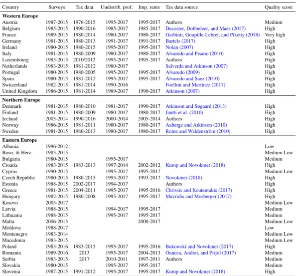
Sources We collect and harmonize household survey data from several interna-tional and country-specific datasets. Our most important source of survey data is the

11_{We link together the various series, rescaling older and lower-quality series to match the newer} and higher-quality ones in their latest year of overlap to avoid any structural break.

12_{Using these sources, we have a sufficiently detailed decomposition of national income that} covers nearly 100% of the continent national income up until 1995. Before that, coverage becomes increasingly sparser: we have the full decomposition for about 50% of national income in 1990, decreasing to 20% at the very beginning of our series. We impute missing series by retropolating them using exponential smoothing with a coefficient of 0.9. As a last resort, we rely on regional averages.

13_{The DINA guidelines (Alvaredo et al., 2016) distinguish between social insurance benefits (D621} + D622 in the SNA) which individuals are entitled to if they have contributed and social assistance benefits in cash (D623), which indivudals can receive without having contributed. Unfortunately that level of details is not commonly available in the national accounts of most countries, which only report the aggregate item D62. This is why we rely on alternative sources.

European Union Statistics on Income and Living Conditions (EU-SILC), which have been conducted on a yearly basis since 2004 in thirty-two countries. We complement EU-SILC by its predecessor, the European Community Household Panel (ECHP), which covers the 1994-2001 period for thirteen countries in Western Europe. Our second most important source of survey data is the Luxembourg Income Study (LIS) that provides access to harmonized survey microdata covering twenty-six countries since the 1970s. Most Western European countries are covered from 1985 until today, and several countries from Eastern Europe have been surveyed since the 1990s. Imputations When we have access to survey microdata, we can usually estimate income concepts that are close to our concepts of interest (pretax and posttax income) with only a few components of income that remain to be added separately (see

sec-tionIV.E.). A significant exception concerns social contributions in EU-SILC: while

both employer and employee social contributions are recorded, employee contribu-tions are combined with income and wealth taxes. We use the social contribution schedules published in the OECD Tax Database to impute employee social contri-butions separately. Before 2007, employer contricontri-butions may also not be recorded despite having information on income before taxes and employee contributions. In such cases, we also impute employer contributions based on schedules from the OECD Tax Database. Beside that, measures of income before and after taxes and transfers have been recorded consistently as part of EU-SILC. The Luxembourg Income Study also produces some historical data on pretax income, in many cases by imputing direct taxes and social contributions as part of their harmonization effort. As a result, we have survey microdata on both pretax income and posttax income in almost all countries since 2007, and for over a longer time period for a number of Western European countries (Germany, the United Kingdom, Switzerland, and Nordic countries).

IV.C. Survey Tabulations

Sources We complement the survey microdata with a number of tabulations avail-able from the World Bank’s PovcalNet portal, the World Income Inequality Database (WIID) and other sources. PovcalNet provides pre-calculated survey distributions

by percentile of posttax income or consumption per capita. The WIID gathers in-equality estimates obtained from various studies, and gives information on the share of income received by each decile or quintile of the population. Finally, we collect historical survey data on posttax income inequality in former communist Eastern European countries provided byMilanovic (1998). In all cases, we use generalized Pareto interpolation (Blanchet, Fournier, and Piketty, 2017) to recover complete distributions from the tabulations. A detailed breakdown of available survey data sources by country is available in the extended appendix.

Harmonization Contrary to microdata, tabulations only provide distributions cov-ering specific income concepts and equivalence scales. The majority of tabulations recorded in PovcalNet and WIID correspond to posttax income, while cases in which we only observe consumption are limited to a handful of Eastern European countries (Moldova, Kosovo, Montenegro).14 _{The equivalence scales available}

are more diverse, including households, adults, individuals, the OECD modified equivalence scale or the square root scale.15 _{For these data sources, as well as for}

survey microdata where information on taxes and transfers is incomplete, we have to develop a strategy to transform the distribution of the observed “source concept” (e.g. consumption per capita or posttax income among households) into an imputed distribution measured in a “target concept” (pretax or posttax income per adult).

The key idea behind our harmonization procedure is that, while the different income or consumption concepts that we observe are different, they are also related. Using all the cases where the income distribution is simultaneously observed for two different concepts, we can map the way they tend to relate to one another, and use that to convert any source concept to our concept of interest. In practice, we formalize this idea by writing the average income of each percentile for the 14_{The only exceptions correspond to a handful of Eastern European countries at the beginning} of the period (Bosnia and Herzegovina, Moldova, Montenegro) for which we have no other source available. In these cases we use the survey distribution of pretax income as a proxy for the “true” pretax income.

15_{When computing inequality estimates with the OECD modified equivalence scale, the first adult} in the household is given a weight of 1, other adults are given a weight of 0.5, and children are given a weight of 0.3 each. The square root scale divides total income by the square root of the size of the household.

distribution of interest as a function of all the percentiles of the distribution from which we wish to impute, and also as a function of various auxiliary variables that may potentially account for that relationship (average income, population and household structure, marginal tax rates, social expenditures). Finding that function amounts to a regression problem, albeit a high-dimensional, non-parametric one. To avoid making ad hoc restrictions, we rely on recent advances in non-parametric high dimensional statistics, also known as machine learning. We use XGBoost (Chen

and Guestrin, 2016), a state-of-the-art implementation of a standard, robust and high

performing algorithm called boosted regression trees. We provide a detailed view of the method and the results in sectionI.A.of appendixA. In particular, we show that this approach performs better than more naive ones, such as assuming a single correction coefficient by percentile, especially in countries where we have to resort to poor predictors of income, such as consumption.

Still, we stress that this approach is not perfect: the relationships between the different concepts are not deterministic, so that these imputations involve their share of uncertainty. However, the existing literature has often chosen to ignore these issue altogether, and directly combined, say, income and consumption data (e.g.Lakner

and Milanovic, 2016). We feel that our approach is preferable, because it corrects at

least for what can be corrected. Note that in the end, the output of the harmonization procedure is straightforward and intuitive: it mostly adjust the levels of the different series, but does not introduce any trend that was not already in the data. We show the impact of these corrections country by country in our extended appendix. IV.D. Survey Corrections

Survey data are known to often miss the very rich. For our purpose it is important to distinguish two reasons for that: non-sampling and sampling error. Sampling error refers to problems that arise purely out of the limited sample size of survey data. Low sample sizes affect the variance of estimates, but they may also create biases, especially when measuring inequality at the top of the distribution. Non-sampling error refers to the systematic biases that affect survey estimates in a way that is not directly affected by the sample size. These mostly include people refusing to answer surveys and misreporting their income in ways that are not observed, and therefore

not corrected, by the survey producers. Estimates based on raw survey data do not account for any of these biases and therefore tend to underestimate incomes at the top end.

Non-sampling Error We correct survey data for non-sampling error using known top income shares estimated from administrative data. Following contributions by

Piketty (2001)for France andPiketty and Saez (2003)for the United States, several

authors have been using tax data to study top income inequality in the long run. Most of these studies have been published in two collective volumes (Atkinson and

Piketty, 2007;2010), and their results have been compiled in the World Inequality

Database.16 _{In general, tax data is only reliable for the top of the distribution, and}

this is why these series do not cover anything below the top 10%. In that literature, researchers estimate the share of top income groups by dividing their income in the tax data by a corresponding measure of total income in the national accounts. At the time of writing, data series were available for nineteen European countries, providing information on the share of income received by various groups within the top 10%.

We complete this database by gathering and harmonizing a new collection of tabulated tax returns covering Austria (1980–2015), East Germany (1970–1988), Estonia (2002–2017), Iceland (1990–2016), Italy (2009–2016), Luxembourg (2010, 2012), Portugal (2005–2016), Romania (2013) and Serbia (2017). We use these tabulations to add new top income shares to our database. We provide a detailed account of the computations for each country in the extended appendix. In most cases, we directly correct the surveys with the tax data using the method ofBlanchet,

Flores, and Morgan (2018)rather than using a total income estimate from the national

accounts. Direct correction of survey data is a more flexible and practical approach, at least for the recent period, and is now being preferred in the latest work on inequality (e.g.Bukowski and Novokmet, 2017;Morgan, 2017;Piketty, Yang, and

Zucman, 2019). When extending existing series using that method, as in Italy or

Portugal, our results are consistent with the work that was done previously, thus confirming the consistency and reliability of both approaches. Our results also reveal

that the underestimation of top incomes varies a lot across surveys and is typically higher in Eastern European countries. This points to the importance of correcting surveys with tax data to make comparisons between countries more reliable.

We correct the survey data using standard survey calibration methods. The principle of survey calibration is to reweight observations in the survey in the least distortive way so as to match some external information. Statistical institutes already routinely apply these methods to ensure survey representativity in terms of age or gender. We directly extend them to also ensure representativity in terms of income. The applicability of these methods to correct for the underrepresentation of the rich in surveys has been discussed at length byBlanchet, Flores, and Morgan (2018).

One difficulty is that our external source of information consists in top income shares. Because top income shares are a non-linear statistic, they cannot directly be used in standard calibration procedures. We tackle that issue using suggestions from

Lesage (2009). They involve linearizing top income shares statistics by calculating

their influence function, and introducing a nuisance parameter. We discuss that methodology in detail in appendixA. In concrete terms, we increase weight at the top of the distribution so that survey top incomes match their value observed in the tax data.

One advantage of calibration procedures is that they allow to perform survey correction with a taxable income concept that may differ from the income concept of interest — either in terms of income definition or statistical unit. We always match concepts to the best of our ability between the tax data and the survey data to perform the correction. Then we use income concepts that are better defined and more economically meaningful to produce our inequality series. Confronting tax data and survey data as such is a very powerful way to make income tax statistics comparable between countries.17 _{It lets us account for top incomes while retaining}

the wealth of information included in the surveys, notably on taxes and transfers, so

17_{For older time periods from which we cannot perform that exercise directly due to lack of proper} survey microdata, we retropolate the correction on the income tax series that is done over the more recent period. See extended appendix for details.

that we can study them and calculate both pretax and posttax incomes.18

When we do not directly observe tax data in a country, we still perform a cor-rection based on the profile of nonresponse that we observe in other countries. This is only the case for a few small countries — Albania, Bosnia and Herzegovina, Bulgaria, Cyprus, Kosovo, Latvia, Lithuania, Macedonia, Malta, Moldova, Montene-gro and Slovakia. To capture statistical regularities, we estimate the nonresponse profile as a function of the distribution of income in the uncorrected survey using the same machine learning algorithm as in sectionIV.C.. We stress that this remains a rough approximation and that in our view the proper estimation of top income inequality requires access to tax data. Fortunately, our tax data covers the majority of the European population, and an even larger share of European income, so that the impact of these corrections on our results is small. Indeed, as shown in figure A.2.11 in appendix, excluding these countries from the analysis has little impact on the results.

Sampling Error The sample size of surveys varies a lot and can sometimes be quite low: this, in itself, can seriously affect estimates of inequality at the top and, on average, will underestimate it (Taleb and Douady, 2015). Correcting sampling error requires some sort of statistical modeling. We borrow methods coming from extreme value theory, which is routinely used in actuarial sciences to estimate the probability of occurrence of very rare events, but can similarly be used to estimate the distribution of income at the very top.

The main tenet of extreme value theory is that a parametric family of distribu-tions — the generalized Pareto distribution — more or less provides a universal approximation of distribution tails. It is a flexible model and includes the Pareto, the exponential, or the uniform distribution as a special case. We use it to model the top 10% of income distributions. We estimate the model using a simple and robust method known as probability-weighted moments (Hosking and Wallis, 1987). We 18_{Our ability to explore the composition of top incomes is still limited by the precision of the} survey data. At the European level and over several years, the number of observations is sufficient to study the top 1%, but not much higher. When it comes to studying the marginal distribution of pretax and posttax incomes, however, statistical methods can address these sampling error issues (see below).

provide technical details for the method in appendixA. Note that by construction, this adjustment has absolutely no impact on the top 10% income share (which we know from the tax data), it only refines the income distribution within the top 10%. IV.E. Incomes Traditionally Excluded from Tax and Survey Sources

Once we have harmonized and corrected our survey data using tax data, we find ourselves with more correct and comparable inequality series. But those series do not yet account for all of the national income because they lack some components from the household sector (imputed rents), the corporate sector (undistributed profits) and the government sector (taxes on products and government spending).19

Imputed Rents We extract the total value of imputed rents from the national accounts. To distribute them, we rely on (calibrated) EU-SILC data that does record imputed rents (although they are not included in the headline inequality figures). We perform a simple statistical matching procedure using income as a continuous variable to add imputed rents, which we describe in the appendixI.D.. The imputed rents total is rescaled to match national accounts. The method preserves the rank dependency (i.e. the copula) between income and imputed rents in EU-SILC, the distribution of imputed rents in EU-SILC, the distribution of income in the original data, and the imputed rents total in the national accounts.

Undistributed Profits We distribute the private share of undistributed profits to individuals proportionally to the ownership of corporate stock. This includes both private and public stocks that are held directly or indirectly through mutual funds and private pension plans. However, we exclude sole proprietorship, since in the national accounts they are not an entity separate from the household to which they belong.20

19_{Some minor discrepancies remains (government surplus, FISIM, NPISH income, etc.). Given} the size of these aggregates, they can only have minor impacts on the overall distribution. We distribute them proportionally. The DINA guidelines (Alvaredo et al., 2016) sometimes suggest slightly more refined imputation methods, but these are more difficult to apply given the nature of our data, and have only very limited impact on the results.

20_{This income is part of “mixed income” and distributed as part of the rest of household sector} income.

The amount of undistributed profits comes from the national accounts. We determine the share of these profits that is privately owned (rather than government-owned) using the financial balance sheets: we calculate the share of equity assets that is owned by the household sector out of the equity assets owned by both the household and the government sector. Government-owned undistributed profits are treated like a primary income of the government.

The distribution of stock ownership comes from the Household Finance and Consumption Survey (HFCS), the pan-European wealth survey of the European Central Bank. We calibrate that survey on the top income shares as we do for other surveys to make it representative in terms of income and to get consistent results. The HFCS only started around 2013, so before that year we keep the distribution of retained earnings constant and only change the amount of retained earnings to be distributed: this constitutes a reasonable approximation because stock ownership is always highly concentrated, so that the main impact of retained earnings on inequality comes from changes in their average amount rather than changes in the inequality of stock ownership. After 2013, we use the wave that is closest to the year under consideration.

The Corporate Income Tax Because the corporate income tax is paid out of corporations’ profit, we distribute it similarly to undistributed profits in pretax income.

Taxes on Products and Production In our benchmark series we distribute taxes on products and production proportionally to pretax income, so we do not need any additional source. But we provide alternative series in which taxes on products are distributed proportionally to consumption (see figure A.2.4 in extended appendix). For that, we rely on the Household Budget Surveys (HBS) from Eurostat to get the distribution of consumption and its dependency to income. We use the same statisti-cal matching procedure as before to attribute a consumption to people alongside the income distribution, and attribute the taxes on products proportionally to it.

In-kind Transfers We distribute public health spending in a lump-sum way to individuals. That is, we assume that healthcare that is free at the point of use provides an insurance value that is the same for everyone across the population. We distribute other types of in-kind transfers proportionally in our benchmark series, similarly to earlier DINA studies (Piketty, Saez, and Zucman, 2018).

IV.F. Validation of our Methodology

The Impact of the Different Methodological Steps Our estimates differ from existing, survey-based estimates for two groups of reasons: because we use tax data at the top of the distribution, and because we incorporate forms of income that are traditionally absent from inequality statistics. How do these elements impact our results? FigureIagives the answer.21 _{Based only on raw, survey-based estimates,}

we would conclude that inequality has been slightly going down in Europe after a one-time increase in the early 1990s: the top 10% income share has been stable after 1995, while the bottom 50% income share has been slightly but consistently on the rise. When using tax data to correct the top of the distribution, we get a fairly different picture: the increase of the top 10% income has been much more significant, while the share of the bottom 50% has been stable. Adding missing income components modifies the distribution of income further. Some income components (such as undistributed profits) have a strong unequalizing impact, while others (like imputed rents) have more equalizing tendencies. Overall, we distribute between one fifth and one quarter of national income in the form of additional income components. This leads to our “DINA” series, which show a slightly higher top 10% income share in recent years than survey and tax data alone. Most of the difference with raw survey estimates, however, comes from tax data.22

[Figure 1 about here.]

Comparison with Earlier Works We wish to provide results that are conceptu-ally similar to other works on distributional national accounts (Bozio et al., 2018;

21_{Our extended appendix shows the impact of the different steps country-by-country.}

22_{We provide a similar reconciliation of our results with official Eurostat data in figure A.2.2 of} the extended appendix.

Garbinti, Goupille-Lebret, and Piketty, 2018;Piketty, Saez, and Zucman, 2018). But in practice our methodology is quite different. In France,Garbinti, Goupille-Lebret,

and Piketty (2018)andBozio et al. (2018)estimated the distribution of pretax

na-tional and posttax disposable income using detailed tax microdata, combined with various surveys, microsimulation models for taxes and benefits, rescaling income component by component to the national accounts. We, on the other hand, only use tax tabulations to correct survey data, and rescale our results to the national accounts at a coarser level. The advantage of our method is that it is applicable much more widely and rapidly, including in countries in which no tax data is available.

To what extent can our approach yield results that are comparable to more complex and detailed works? As figureIbshows, we get results that are very similar to these earlier works in the case of France (see the extended appendix for detailed information on French data sources and methodological steps). Concretely, our methodological approach starts from the raw survey series shown on the bottom line, which suggest that the top 10% share has fluctuated between 22% and 26%. In a second step, we calibrate these distributions to the fiscal income shares measured from tax data, which reveal that this share has in fact remained approximately constant over time, reaching about 30%. In a third step, we impute additional sources of income, such as retained earnings and imputed rents. This gives us the DINA top 10% pretax income share, which follows closely the series estimated by

Garbinti, Goupille-Lebret, and Piketty (2018). Finally, we impute all taxes, as well

as cash transfers. This yields the distribution of posttax disposable income, which is also remarkably similar to that obtained byBozio et al. (2018).23 _{Note that we}

obtain these results in spite of the fact that our data sources for France are not of an especially high quality — and are also very different from the ones used in DINA

23_{We show in figure A.2.10 in appendix that we also closely reproduce those studies’ findings for} the bottom 50% of the distribution.

projects.24

V. THE DISTRIBUTION OFEUROPEAN NATIONAL INCOMES, 1980-2017

In this section, we show that pretax inequality has risen much less in Europe than in the US since 1980. This is true for most European countries taken separately but also for Europe taken as a whole — a block that is broadly similar in terms of population size and aggregate economic output as the US.25

V.A. The distribution of pretax income in 2017

TableIshows the average incomes of various groups in Western and Northern Europe, Eastern Europe and the United States for comparison. Regional differences between Western Europe Northern Europe and Eastern Europe are mainly driven by differences among bottom income groups rather than by differences at the top of the distribution. The average income of Western and Northern Europeans is about 80% higher than the average income of Eastern Europeans. When comparing the incomes of the poorest 20% of adults in these regions, however, this gap exceeds 250%. Accordingly, tableIreveals a remarkable degree of convergence in the top incomes of Western Europe, Northern Europe and Eastern Europe. The top 0.001% earns close to 9 million euros in Eastern Europe, compared to just above 10.5 million euros in Western and Northern Europe.

[Table 1 about here.]

24_{The SILC statistics for France are a transcription of a survey (called SRCV) which is used for} its extensive set of questions on material poverty, but is not considered the best survey for income inequality. For that purpose, the French statistical institute relies on another survey, called ERFS. But that survey is not part of any international scheme, such as EU-SILC, nor is it available through portals such as the Luxembourg Income Study. Therefore, we do not include it in our estimations. Before SILC is available, we rely on France’s Household Budget Survey, which has been made available through LIS. While France’s HBS is a key source for consumption data, it is not viewed a the best source for income data either. It is also separate from EU-SILC data, which explains the inconsistent trend. Therefore, there is no reason to think that our methodology would work better for France than other countries just because of the quality of the data in input.

25_{In 2018, aggregate national income was e14.2tn in Europe and e13.1tn in the US. Total} population was 432 million in Europe and 241 million in the US. In terms of population, Western and Northern Europe combined (334 million) are more comparable to the US than Europe as a whole. See Appendix TableA.6for the composition of Europe and its subregions).

On the other hand, income differences between Europe and the United States are mostly driven by top incomes. The average national income per adult in the United States is 45% higher than in Western and Northern Europe, and more than 2.5 times higher than in Eastern Europe. Yet, the bottom 50% of the US population earns 15% less than the bottom 50% of Western and Northern Europe, and more than 40% less when looking at the bottom 20%. By contrast, the average pretax income of the top 1% exceeds one million euros in the United States, compared to e372,000 in Western and Northern Europe and e238,000 in Eastern Europe.

V.B. The rise of top incomes

[Figure 2 about here.]

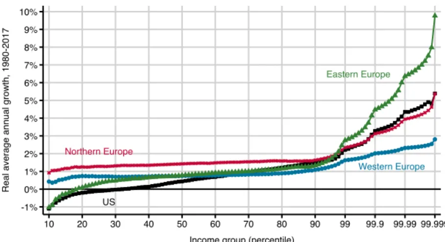
FigureIIshows the evolution of the pretax income distribution between 1980 and 2017 in Western Europe, Northern Europe, Eastern Europe and the US, with a further decomposition of groups within the top 1%. In all three European regions, growth has been markedly higher for the top 10% than for the bottom 90% of pretax income earners, and has been even higher at the very top of the distribution. The distribution of growth has been much more skewed in Eastern Europe than in the rest of the continent.26 _{In the US, the bottom 50% did worse than its counterparts in}

all European regions.

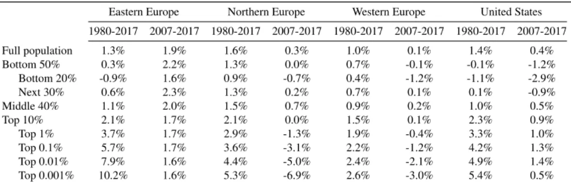
V.C. The distribution of macroeconomic growth [Table 2 about here.]

TableIIshows the average annual real pretax income growth of selected income groups in Western Europe, Northern Europe, Eastern Europe and the United States over the 1980-2017 and 2007-2017 periods.

26_{Let us stress here that we focus solely on monetary income inequality, which was unusually low} in Russia and Eastern Europe under communism. Other forms of inequality prevalent at the time, in terms of access to public services or consumption of other forms of in-kind benefits, may have enabled local elites to enjoy higher standards of living than what their income levels suggest. That being said, the survey tabulations at our disposal do partially account for forms of in kind income, so this limitation should not be exaggerated (seeMilanovic, 1998). Furthermore, the top 10% income share did continue to rise in many Eastern European countries after 1995 and is now higher than in other European regions.

While the long run picture reveals a clear increase in inequality, the period of stagnation that followed the 2007-2008 crisis has been less detrimental to the European middle class than to other income groups. In Western Europe and Northern Europe the average incomes increased for groups located at the middle of the distribution more than for any other groups. Eastern European countries were less affected by the crisis but experienced comparable evolutions: the bottom 20% grew at an annual rate of 1.6% between 2007 and 2017, lower than the regional average of 1.9%. Therefore, while the financial crisis has to some extent halted the rise in top income inequality in Europe, income gaps between the middle and the bottom of the distribution have continued to widen, and low incomes have consistently lagged behind the expansion of the overall economy.

The distribution of growth in the United States since 2007 has been unambigu-ously more skewed: the average national income grew faster than in Western and Northern Europe at an annual rate of 0.4%, but the pretax incomes of the bottom 50% dropped by 1.2% and that of the bottom 20% by as much as 2.9%.

V.D. The role of regional integration and spatial inequality [Figure 3 about here.]

The top panel of figureIIIcompares the levels and evolution of the top 1% and bottom 50% income shares in the US, Europe as a whole, and Western and Northern Europe between 1980 and 2017.27 _{Income inequality was unambiguously larger}

in the US than in Europe in 2017, even after accounting for differences in average incomes between European countries. The share of regional income received by the top percentile was twice as high in the United States (21%) as in Western and 27_{We choose to pool together Western and Northern Europe because of their similarities in} terms of political institutions (most countries joined the EU by the mid-1990s), living standards and economic tax and transfer systems (as discussed in the next section). For Europe as a whole, as well as for Northern and Western Europe, we aggregate country-level distributions after converting average national incomes at market exchange rates euros, rather than at purchasing power parity. This approach is justified by the fact that PPP conversion factors exist for European countries but not for US states: it would be unclear why one would correct for spatial differences in the cost of living in the former case but not in the latter. Estimating the distribution of European-wide income at purchasing power parity slightly reduces European inequality levels, as well as the share of inequality explained by between-country income disparities, so it does not affect our main conclusions.

Northern Europe (10.5%) or even Europe at large (11%). Meanwhile, the income share of the bottom 50% reached 16% in Europe and 20% in Western and Northern Europe as compared to less than 12% in the US. This was not always the case: in 1980, the bottom 50% share was actually higher in the US than in Europe as a whole, amounting to 20% of the national income, and it was only two percentage points lower than in Western and Northern Europe.

A more detailed picture of the distribution of growth in Europe and the US is shown in the bottom panel of figureIII, which plots the average annual income growth by percentile in the two regions between 1980 and 2017, with a further decomposition of the top percentile. Growth of the average national income per adult was slightly higher in the US than in Europe: it exceeded 1.35% per year in the former, compared to 1.14% in the latter. However, this average gap hides important differences across the distribution. The average pretax income of the top 0.001% grew at a rate of 3.25% in Europe as a whole and as much as 5.39% per year in the US.28 _{Meanwhile, macro growth has benefited significantly more to low-income}

groups in Europe than in the US.

[Figure 4 about here.]

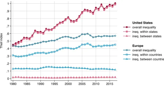
To what extent are these figures driven by differences in average incomes between US states and between European countries, rather than within states and within countries? A Theil decomposition of within-group and between-group inequality in Europe and the US is shown in figureIV. The Theil index has risen much more in the US than in the Europe, and this change has been entirely due to increases in inequality within US states. In 1980, the Theil index in the US was almost perfectly equal to that of Europe at large, amounting to about 0.45; in 2017, by contrast, it was higher than 1 in the US, whereas it did not exceed 0.6 in Europe. The overall Theil index and the Theil index of within-state inequality are almost indistinguishable in the US: within-state inequality explained 97% of overall US inequality in 1980, and as much as 99% in 2017. The share of inequality explained by the between-group component is larger in Europe, but it has decreased from about 30% in 1980 to 20% in 2017, due to the rise in income differences within countries. In other

words, average income convergence in Europe has become increasingly insufficient to reduce inequalities between European residents.

VI. THEIMPACT OFTAXES AND TRANSFERS ONINEQUALITY

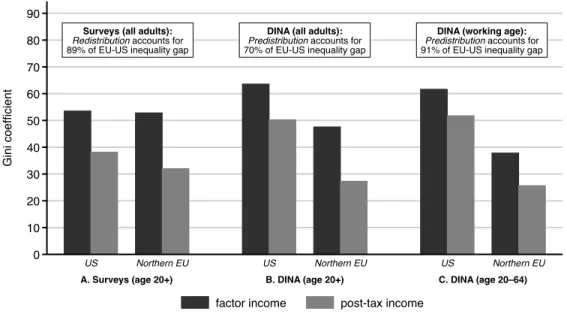
Our findings suggest that taxes and transfers are not more redistributive in Europe than in the US. However, given the higher level of pretax inequality in the US, European countries remain more equal than the US after all taxes and transfers are taken into account. Defining predistribution as the entire set of policies and institutions impacting the distribution of pretax incomes, and redistribution the entire set of policies impacting the distribution of posttax incomes, we find that Europe is more equal than the US thanks to predistribution rather than redistribution, contrary to a widespread view.29

VI.A. The Structure and Distribution of Taxes

We start from the aggregate value of taxes and transfers available in National accounts. Appendix table A.4 and section B present these values for the three European regions and for the US, with a break-down by type of taxes and transfers. We now seek to distribute all these taxes (including corporate, sales and value-added taxes) paid by the different income groups.

In what follows, we distinguish two ways to report total taxes paid by income groups: (i) non-contributory taxes paid as a share of pretax income (i.e. excluding social contributions that pay for social insurance schemes) and (ii) total taxes paid as a share of factor income. When presenting taxes paid as a share of pretax income, we remove contributory social contributions from the analysis, since our definition of pretax income is net of the operation of pension and unemployment insurance systems. This way to look at tax incidence is useful for international comparisons focusing on the entire support of the adult distribution (i.e. when looking at the working and non-working populations). Its downside is that it misses a share of payments that can legitimately be considered as taxes by individuals. In countries 29_{See for instanceOECD, 2008;2011who reach the opposite conclusion as we further discuss} below. See alsoHacker (2011)for a discussion of predistribution and redistribution.