Workplace smoking ban effects in an heterogeneous smoking population

(1)

HAL Id: halshs-00564896

https://halshs.archives-ouvertes.fr/halshs-00564896

Preprint submitted on 10 Feb 2011

HAL is a multi-disciplinary open access archive for the deposit and dissemination of sci-entific research documents, whether they are pub-lished or not. The documents may come from teaching and research institutions in France or abroad, or from public or private research centers.

L’archive ouverte pluridisciplinaire HAL, est destinée au dépôt et à la diffusion de documents scientifiques de niveau recherche, publiés ou non, émanant des établissements d’enseignement et de recherche français ou étrangers, des laboratoires publics ou privés.

Workplace smoking ban effects in an heterogeneous

smoking population

Clément de Chaisemartin, Pierre-Yves Geoffard

To cite this version:

Clément de Chaisemartin, Pierre-Yves Geoffard. Workplace smoking ban effects in an heterogeneous smoking population. 2010. �halshs-00564896�

(2)

WORKING PAPER N° 2010 - 21

Workplace smoking ban effects

in an heterogeneous smoking population

Clément de Chaisemartin Pierre-Yves Geoffard

JEL Codes: C21, I12, I18

Keywords: Workplace smoking ban, tobacco control, smoking cessation, impact evaluation

P

ARIS

-

JOURDAN

S

CIENCES

E

CONOMIQUES

48,BD JOURDAN –E.N.S.–75014PARIS TÉL. :33(0)143136300 – FAX :33(0)143136310

www.pse.ens.fr

(3)

Workplace smoking ban effects in an heterogeneous smoking population

Corresponding author:

Clément de Chaisemartin

Paris School of Economics, 48 boulevard Jourdan, 75 014 Paris, France

chaisemartin@pse.ens.fr

Phone number: 0033143136364

Author:

Pierre-Yves Geoffard

Paris School of Economics, 48 boulevard Jourdan, 75 014 Paris, France

geoffard@pse.ens.fr

5 774 words.

JEL code: C21, I12, I18

Acknowledgements:

We are very grateful to Anne-Laurence le Faou for providing us the database of French cessation services, as well as to Paul Dourgnon and Thierry Debrand at the Institute for Research and Information in Health Economics (IRDES), who gave us access to the ESPS survey.

(4)

Abstract

Many public policies, and especially health policies, are aimed at modifying individual behavior. This is particularly true of anti smoking policies. However, health behavior is highly heterogeneous, and so are individual responses to public policies such as taxes or restriction on use. We investigate the effect of a workplace smoking ban which took place in France in 2007. By its national aspect, the French reform offers a good case to study the effect of workplace smoking bans. Using original data on patients who consult tobacco cessation services, we show that the ban caused an increase in the demand for such services, and in the number of successful attempts to quit smoking. However, using survey data, we show that the ban had no measurable effect on overall prevalence in the general population. Models of quasi rational smoking behavior may offer an explanation for these two apparently contradictory findings.

(5)

1 Introduction

Along positive effects on passive smoking (Callinan et al., 2010), workplace smoking bans have been credited for a drop in smoking prevalence. A meta-analysis of 26 papers found that workplace smoking bans reduce smoking prevalence by 3.8 percentage points (Fichtenberg and Glantz, 2002). However, all of these 26 papers study the impact of smoking bans voluntarily implemented in some specific workplaces, but not in all (“voluntary bans”). Several studies are based on cross-sectional analyses which compare smoking prevalence in workplaces with differing smoking policies (Evans et al., 1999). Other use longitudinal data and compare the rate of smokers among employees of one particular workplace before and after a ban (Stave and Jackson, 1991).

But two phenomena raise endogeneity issues: feasibility of a local ban, and endogenous job choice. Firstly, simple political economy considerations suggest that voluntary bans are most likely to be passed in firms with the lowest proportion of smokers, which would weaken the relevance of cross-sectional comparisons. Secondly, assortative matching between firms and workers could entail a drop in smoking prevalence within a specific workplace following a voluntary ban, without implying any general population drop. Indeed, after a ban is enacted in a given firm, smokers might choose to leave this firm, and newly hired employees are more likely to be non smokers. Therefore, longitudinal analysis of voluntary bans might be biased as well. Evans et al. (1999) try to circumvent these potential endogeneity biases through an IV estimate. Their instrument for voluntary ban is the number of employees in the workplace which they find to be highly correlated to the presence of a ban. Still, the exogeneity of their instrument is questionable. Indeed, employees in smaller firms differ from those in larger ones on many observable characteristics (Headd, 2000), so that they could also differ on unobserved characteristics related to their smoking behavior.

(6)

In the case of a nationwide smoking ban which applies to all firms (“compulsory ban”), the assortative matching effect, as well as the political economy one, is absent. Indeed, a compulsory ban is exogenous, insofar as it is not anticipated and that firm compliance to the regulatory change is high. A recent meta-analysis (Callinan et al., 2010) included 15 studies considering the impact of legislative bans on smoking and reported mixed evidence. 9 studies found a negative impact of the ban whereas 6 studies found no impact. However, most of them suffer from various limitations. Firstly, the majority of them considered comprehensive bans, that is to say bans in all public places, so that it is impossible to attribute what is

specifically due to the workplace ban. Moreover, all of them are before-after studies but few had a control group or controlled for pre-existing temporal trends in smoking prevalence.

In 2005, 30% of the French population was smoking (Beck et al., 2007) and tobacco was the first cause of preventable death, causing 66 000 deaths per year (Hill and Laplanche, 2003). Workplace passive smoking has been reported to cause 617 deaths annually in the UK (Jamrozik, 2005) even though one study found a lower estimate for France (Alipour et al., 2006). To tackle this issue, a first law was passed in 1991, which prohibited smoking from collective areas in workplaces (meeting rooms…) but obliged employers to set up specific areas where smoking was allowed. It was poorly enforced (Baudier and Arènes, 1997). Therefore, a national level comprehensive workplace smoking ban was promulgated on the 15th of November 2006 and became effective in February 2007. It banned smoking from all areas in workplaces, and prohibited the implementation of specific areas where smoking was allowed, unless they meet several restrictive criteria (automatically closing doors…).

The French workplace smoking ban is a good natural experiment to measure the impact of workplace smoking bans on smoking behaviors. Firstly, as is to be seen in Table 1, the enforcement of the ban was good. It indeed appears from a survey conducted by 148 occupational health doctors that 82% of their patients worked in a fully smoke free

(7)

environment after the ban became effective (90% among those working in offices). Moreover, there is both a clear cut-off date and a natural control group: the non working population1. This enables us to measure the impact of the ban through a difference in

differences (DID) identification strategy2 (Abadie, 2005). Finally, the price of cigarette packs remained almost constant between 2004 and 2008 (a 6% increase happened in August 2007).

[Table 1 inserted here]

Our main finding is that the French ban had a heterogeneous impact on different populations of smokers: it increased the number of patients consulting cessation services who have been reported to be heavy smokers but had no impact on French prevalence.

The remainder of the paper in organized as follows. In section 2, we focus on a

specific subset of the French population of smokers: those consulting cessation services. They have been reported to be heavy smokers: 37% of them suffer from tobacco related diseases such as chronic obstructive pulmonary disease, and they smoke more than 20 cigarettes per day on average (Le Faou et al., 2005, Le Faou et al., 2009). The ban increased the number of patients consulting those centers by 24% and the rate of successful quits by 18%. In section 3, we analyze general population surveys and find no impact of the ban on overall prevalence. This suggests that it had no sizeable effect on French “average” smokers hence the absence of impact on overall prevalence, but it incentivized and helped the most intensive smokers to quit. Section 4 sketches a theoretical discussion to rationalize these two contradictory findings and concludes.

1

We exclude children and students from the non-working population since smoking was banned from schools and universities in February 2007 as well.

2

Our DID identification strategy implies that all our regression equations are linear and are estimated with least square techniques, even though our main dependant variable, smoking status, is binary. As a robustness check, we estimate all our regressions with Probit models. This does not change the results as far as the significance of the coefficients of interest is concerned.

(8)

2 The impact of the ban on patients consulting smoking cessation services

2.1 Data and Methods

Data set

We use the data base of French cessation services participating in the “Consultation Dépendance Tabagique” program (hereafter referred to as CDT). This program started in 2001 and led to the progressive implementation of smoking cessation services nationwide. This data set contains a large number of variables. During patients’ first visit, smoking status is evaluated according to daily cigarettes smoked, Fagerström Test for Nicotine Dependence [FTND] (Heatherton et al., 1991) and a measure of expired carbon monoxide (CO) which is a biomarker for tobacco use. At the end of this first visit, treatments may be prescribed to patients (nicotine replacement therapies…). Follow-up visits are offered. Supplementary CO measures are usually made during follow-up visits to validate tobacco abstinence. We study the impact of the ban on the number of new patients consulting per month through a time series analysis and its impact on successful quits through a DID.

Measuring the impact of the ban on the number of new patients consulting per month

To measure the impact of the ban on the number of new patients consulting per month, we must construct our data set. Firstly, most French cessation centers are located in a hospital. They receive both hospitalized patients who are obliged to quit smoking while in hospital, and non hospitalized patients who voluntarily come to seek counseling before making a cessation attempt (Le Faou et al., 2005). We exclude patients who consulted during a stay in hospital. Indeed, their cessation attempt was not voluntary so that we do not expect the workplace smoking ban to have any impact on them. Secondly, since its creation, the program expanded

(9)

from 35 to 116 centers. Therefore, we must select a sample of centers which continuously participated to the program, so that fluctuations in the number of new patients per month cannot be attributed to the opening or closing of centers. Our starting date is 2004: on that year most large centers contributing to the program had already joined. The end date is the last quarter of 2008 where data ends. We include the 45 centers which recorded at least one patient per year into the database from 2004 to 2008. We are left with 27 180 non hospitalized patients who consulted these 45 centers from 2004 to 2008. Finally, since numbers of

employed and not employed new patients consulting per month are not comparable in levels we normalize them to draw a comparison3.

Let Xt be the number of new employed patients consulting cessation centers in month

t and Yt the corresponding figure either for retired, unemployed, inactive or all non

employed patients. X and Y are the normalizers. Our dependant variable is

Y Y X X

Z_t  t  t . It

measures whether the departure from the “normal” number of monthly visits observed in month t was the same for employed and not employed patients. We define a “smoking ban” dummy variable equal to 1 from October 2006 to September 2007 and we estimate

t ban t

Z 1  . ˆ measures the increase in the number of monthly visits, expressed in

percentage of “normal” attendance attributable to the ban.

Measuring the impact of the ban on the rate of successful quits

Our second objective is to measure the impact of the ban on the rate of successful quits by CDT patients. Smoking status assessment is based on CO measures made during follow-up visits. Patients who did not attend a follow-up visit (N=11712) are therefore withdrawn. But some patients only attended follow-up visits very soon after their first visit: we only have

3

We use average attendance from January 2004 to September 2006 and from October 2007 to December 2008 to normalize monthly series (we exclude the period around the smoking ban).

(10)

information on the success of their attempt in the very short run. To deal with this issue we adopt two strategies. We first withdraw all patients who did not attend a follow-up visit more than 57 days (9th week) after their initial visit (N=7 427). 57 days is usually regarded as long enough so that cessation status at that time is indicative of long-run status: in clinical trials of new smoking cessation drugs, cessation rates are generally computed from 9th week onwards (Gonzales et al., 2006). We end up with a sample (hereafter referred to as Selected Sample 1) for which we have reasonably long run cessation outcomes but which represents 24.1% only of the initial sample, which obviously raises selection issues (see Table 2). Therefore, we also run the same analysis on a second sample (hereafter referred to as Selected Sample 2) into which all patients for whom a CO follow-up measure is available are included, whenever those measures were made. This allows raising the selection rate to 51.0% at the expense of including patients for whom only a short run cessation outcome is available.

Abstinent patients are those whose last CO measurement among those made between 57 and 365 days after their first visit (hereafter referred to as 57-365 CO) was below 5 parts per million (ppm)4. Our outcome measure for successful quits is a DID of cessation rates. 2006 and 2007 are periods 0 and 1. Employed patients are the treatment group. Our control group is made up of either retired, unemployed, inactive or all not employed patients.

2.2 Results

Descriptive statistics

Descriptive statistics are displayed in Table 3. The whole sample comprises 27 180 individuals, among which 19 410 are employed (71.4%) and 7 770 are not. CDT patients are

4

Threshold CO values usually range from 5 to 10 ppm (Jarvis et al., 1987). We choose the most restrictive threshold after having performed a sensitivity-specificity analysis (Jarvis et al., 1987) among CDT patients.

(11)

middle-aged, employed, educated and highly addicted smokers: they smoke more than 21 cigarettes per day on average, against only 12 among French smokers. 21 cigarettes

corresponds to the 90th percentile of the distribution of daily cigarettes smoked among French smokers (Beck et al., 2007). As expected, employed patients differ from not employed on various observable characteristics (age, educational attainment…). In selected sample 1, patients are older, more educated, more addicted, more likely to be retired and less likely to be unemployed. There is then a potential attrition bias.

In Table 4, we display descriptive statistics on our three samples. When comparing 2006 and 2007 employed patients on 7 observable characteristics, we find only 2 significant differences at the 95% level out of 21 comparisons (7 observable characteristics  3 samples). Regarding not employed patients, we find only one significant difference. Finally, we

compute the 21 corresponding “placebo” DID. 3 are significant at the 95% level, which is greater than 1.05 which would have been expected under the common trend assumption. All of this gives some credit to our DID identification strategy since the two groups did not change much from 2006 to 2007 and did not follow highly significantly different trends on these 7 observable characteristics.

Finally, in selected sample 1 (resp. selected sample 2), CO measures on which status assessment is based were made 164.5 days (resp. 92.0 days) on average after the first visit.

The impact of the ban on the number of new patients consulting cessation centers

Monthly normalized attendance of employed and non employed patients is plotted on Figure 1. Zt is the difference between those two lines. The discrepancies between these two curves are extremely small from January 2004 to September 2006. From October 2006 to

(12)

September 2007, attendance by employed patients sharply peaks 4 times. In the meanwhile, attendance by not employed patients peaks as well but much more modestly. The two curves get close again in the end of 2007.

[Figure 1 inserted here]

In regressions displayed in Table 5, 3 smoking ban dummy coefficients out of 4 are significant. It is marginally insignificant when retired patients are used as a control group (P=0.06). In the first column, we use all not employed patients as controls and the smoking ban coefficient is 0.24, meaning that the ban increased by 24% the number of new employed patients consulting cessation centers from October 2006 to September 2007. As per this measure, the effect of the ban is significantly (P=0.05) lower when we use retired as the control group (+13%) than when we use unemployed (+28%) or inactive (+29%). This might be because the retired population in France increased by 2.6% from 2006 to 2007, whereas the number of unemployed (resp. inactive) decreased by 8% (resp. 3%), while the employed population grew by 2%.

We generate “placebo smoking ban” dummies, that is to say dummy variables equal to 1 during 12 consecutive months before October 2006 (for instance from January 2005 to December 2005). Since the starting point of the analysis is January 2004, we can generate 22 such dummies allowing for overlap. We run the same regression than in Table 5 replacing the true smoking ban dummy by these dummies. None of the placebo coefficients is significantly different from 0 at a 95% degree of confidence.

Finally, to confirm that this surge in attendance by employed patients was indeed due to the ban, we compare the magnitude of this surge in centers located in rainy and cold areas, with centers located in sunnier and warmer areas. A rough cost-benefit analysis of the

(13)

in cold / rainy areas since they must leave their warm offices to go to smoke in the cold or under the rain. As is to be seen in Table 6, in centers located in areas where the number of rainy days in 2007 was higher than the corresponding average in the sample, attendance by employed patients was increased by 37.4% due to the ban, against only 10.6% in centers located in areas where this number was below the average. The difference between these two coefficients is significant (P-value = 0.00). Similarly, lower temperatures, lower number of sunshine hours and higher level of rainfalls are associated to higher increases in the number of patients consulting (even though this last difference is not significant).

[Table 6 inserted here]

This suggests that the smoking ban entailed a surge by 24% in the number of new patients consulting cessation services over 12 months. The fact that this rise started in the end of 2006 might suggest that many firms implemented bans between the moment the law was promulgated and the moment it became effective.

The impact of the smoking ban on the rate of successful quits

In table 7, we display 24 DID estimates (2 samples4 control groups3 models) of the impact of the ban on the rate of successful quits. According to the first regression, in selected sample 1, cessation rate increased by 9.7 percentage points more among employed than not employed patients from 2006 to 2007. When controls are added, this coefficient hardly changes. When only retired patients are used as the control group the DID is no longer significant whereas it becomes even larger with unemployed or inactive as controls.

Including all patients for whom there is a CO measure available (52% of the initial sample) does not substantially change the results. To further control for a potential selection bias, we run the same DID regressions including a first stage equation for selection (Heckman, 1979). After running simple probit models for selection, we choose centres fixed effects as our

(14)

instruments. Indeed, they prove to be highly correlated with patients’ selection status (14 centers have a P-value lower than 0.05 in the probit selection equation). DID hardly change in Heckman selection models.

According to the model without controls, cessation rate among selected and employed patients would have been equal to 53.5% in 2007 without the ban. The estimated effect (9.7 percentage points) therefore represents a 18% increase. The effects estimated are therefore both statistically significant and important.

Identification of the average treatment effect on the treated (ATT) through DID relies on a common trend assumption (Abadie, 2005). Under Rubin’s notations of potential

outcomes (Rubin, 1974), if Y(0) stands for an individual’s smoking status when smoking is not banned in his workplace, and if Y(1) is his smoking status when smoking is banned from his workplace, then common trend assumption can be rewritten as:

) 0 , 0 / ) 0 ( ( ) 0 , 1 / ) 0 ( ( ) 1 , 0 / ) 0 ( ( ) 1 , 1 / Y(0) ( t  e  EY t  e   E Y t  e EY t  e  E .

Here, it means that should there have been no smoking ban, cessation rate would have

followed the same evolution from 2006 to 2007 among employed and not employed patients. To test this assumption, we compute 6 placebo DID estimates along with the true DID in Table 8. None of the 6 placebo estimates is significant at a 5% degree of confidence. One is marginally insignificant (P-value = 0.11), but this is compatible with the fact that when 6 placebo DID are computed you expect to have 1 with a P-value lower than 0.15. Another interesting element is that the 2007-2008 DID is either positive (selected sample 1) or slightly negative (selected sample 2): the impact of the ban on the rate of successful quits has been apparently long lasting. Finally, 2005-2006 DID are negative: we would therefore have obtained even larger estimates had we used a triple differences identification strategy.

(15)

3 The impact of the ban on overall smoking prevalence.

3.1 Data

We use 5 waves (2000, 2002, 2004, 2006 and 2008) of the French Health, Health Care and Insurance Survey (ESPS) carried out every two years by the Institute for Research and Information in Health Economics (IRDES). The survey sample of each wave covers 8 000 households (and 22 000 individuals) randomly drawn from administrative files of the main sickness funds to which over 90% of the French population belong (Allonier et al., 2010).

Data on 30 264 individuals has been collected in 2006 and 2008 (see Table 9). After withdrawing those who did not mail back their questionnaire (N=7 591) and those who did not give their smoking status (N=913), we are left with 21 760 respondents. Then, to construct the “treatment” group, we select employed respondents who are likely to have been affected by the ban. Specifically, we withdraw employed respondents who were on leave at the time of the survey (N=522), whose socio-professional group suggest that they do not work indoor (farmers, tradesmen, shopkeepers, ministers, foremen, domestic staff, skilled and unskilled workers, N=5 490), and who work less than 20 hours per week (N=590). Similarly, to

construct the “control” group, we select not employed respondents who are the most likely not to have been affected by the ban. Specifically, we withdraw non employed respondents who ended working less than one year ago (N=769). We end up with 14 389 observations.

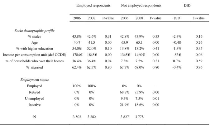
3.2 General population results

(16)

In Table 10, we display descriptive statistics for the 2006 and 2008 samples. Respondents in the 2008 sample are older and the income per consumption unit of their household is higher. Even though the percentage of employed respondents is roughly the same across the two samples, the break-up of the non-working population substantially changes. Among not employed respondents, the share of retired individuals rises by 5.1 percentage points, whereas the share of unemployed and inactive drop. Those trends

mechanically entail a drop in the smoking prevalence of the non working population because retired smoke much less than unemployed and students. This might therefore bias our

estimates of the impact of the ban when we use this population as our control group.5

Even though the sample of respondents is evolving from 2006 to 2008, these changes are not significantly different across employment status groups, for instance across employed and retired respondents. Indeed, none of the 6 placebo DID (Bertrand et al., 2004) we

compute on retired and employed respondents’ observable characteristics is statistically significant, even though the DID on income per consumption unit is only marginally insignificant (P-value = 0.06).

The evolution of smoking prevalence

In Table 11, we display the evolution of smoking prevalence for each employment status group. From 2006 to 2008, hardly any change is to be observed. Employed respondents smoking prevalence insignificantly increased by 0.8 percentage points. Among the non working population, smoking prevalence did not significantly evolve apart among unemployed respondents where it sharply declined. However, due to the change in the

5

One last thing to note is that there are very few unemployed in this sample. This is because 86% of the respondents we withdrew because they stopped working less than one year back were unemployed.

(17)

repartition of the non-working population between retired, unemployed, inactive and students, smoking prevalence among that population diminished by 2 percentage points.

DID analysis

We compute 16 DID, with and without controls, with smoking status or number of cigarettes smoked as the dependant variable and with either the whole non working

population or only retired, unemployed or inactive as the control group. They are displayed in Table 12. The 8 DID estimates for smoking prevalence are positive but only two are

significantly different from 0. In the first regression model, when comparing how smoking prevalence evolved among employed and the non working population, we indeed find that smoking prevalence increased by 2.8 percentage points more (P-value = 0.05) among

employed than among non working respondents. However, as mentioned above, this is mostly due to a composition effect, and as soon as we add controls to the regression, among which subcategories for non working respondents, the coefficient turns insignificant (P-value=0.16). Similarly, when comparing how smoking prevalence evolved among employed and

unemployed, we find a positive DID (P-value = 0.04), which turns insignificant when controls are added. When we compare employed respondents to retired or inactive alone, DID turn insignificant. It therefore seems that the ban had no impact on smoking prevalence. Regarding daily cigarettes smoked, 6 estimates out of 8 are negative, but none is significant. Therefore, the smoking ban had apparently no impact, neither on French smoking prevalence nor on daily cigarettes smoked by smokers.

(18)

To give some support to the common trend assumption on which DID identification relies, we start computing smoking prevalence of the treatment and control groups in the 2000 to 2008 waves of the ESPS survey. They are plotted in Figure 2. The curve of smoking

prevalence among employed respondents is not perfectly parallel to the other curves. Unemployed prevalence rate is extremely volatile, probably due to sample size issues. But smoking prevalence of employed and inactive respondents are almost parallel and always evolve in the same direction from one wave to the other.

[Figure 2 inserted here]

Then, to “test” statistically the common trend assumption, we compute placebo DID, to verify that over years when there has been no workplace smoking ban, smoking prevalence followed similar trends in the treatment and in the control groups (Bertrand et al., 2004). We can perform 3 placebo-wave comparisons: 2000 vs. 2002, 2002 vs. 2004 and 2004 vs. 2006. Multiplied by the four possible control groups, it makes a total of 12 placebo DID, which are displayed in Table 13 along with the 2006-2008 DID. When retired are used as the control group, 2 placebo DID out of 3 are significant at a 90% level. The same is true with

unemployed. This indicates that in this population retired and unemployed respondents are probably not very good control groups for employed respondents. On the contrary, inactive seem to be a valid control group.

A potential confounding factor in our analysis might be labor market dynamics. From 2006 to 2008, only one strong pattern is to be observed: the number of unemployed in France decreased by 300 000 (-12%). Assuming that 100% of these people became employed, this might have resulted in an increase in prevalence among employed from 2006 to 2008 since (former) unemployed smoke more (cf. Figure 2). This could therefore hide the drop in smoking prevalence caused by the smoking ban. Let us make back of the envelope

(19)

computations. Assume that 100% of these 300 000 unemployed people which potentially became employed were smokers in 2008. Assume that the prevalence rate among other employed people remained constant from 2006 to 2008 (27%), which amounts to assuming that the ban had no effect. Under those assumptions, since those 300 000 people only represent 1.2% of 2008 French employed population, prevalence among employed would have been equal to 27.8%, which is what we observe in the data. Therefore, even though this pattern could slightly bias our before-after comparison, it is too small to hide a strong drop in smoking prevalence.

It therefore appears from this analysis that the French smoking ban in the workplace does not seem to have reduced either smoking prevalence or the number of cigarettes smoked by smokers. We also conducted the same DID analysis on the percentage of respondents who made a cessation attempt over the previous calendar year as well as on the percentage of successful quits attempts and we found that the ban had no impact on these variables neither6.

3.3 Are estimates derived from the analysis of voluntary bans biased ?

Since a large body of literature based on voluntary bans concluded that they reduce smoking prevalence, we try to understand where the discrepancy between our “legislative ban” results and those papers arise from. On this purpose, we use a data set collected by 148 French occupational health doctors under the coordination of the French Office for the Prevention of Tobacco (OFT). From January to June 2007, doctors asked the 20 first patients they consulted each month to fill in a short questionnaire. Patients were asked whether smoking was banned in their workplace and their current smoking status. Their age, their sex and a rough classification of their occupation in five categories was also collected, along with some medical information. Data on 13 630 patients have been collected. We exclude 730

6

(20)

patients who work in cafes, restaurants or bars, which are the only workplaces which did not become smoke free on February 1st 2007 (they became smoke free on January 1st 2008), and 41 patients for whom one of variable is missing. We are left with a sample of 12 810 patients.

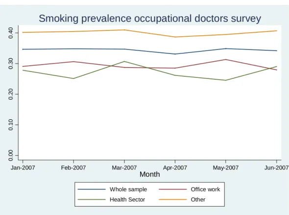
This survey started in January 2007, one month before bans became mandatory. As is to be seen in Table 1, the share of employees working in a smoke free environment was already quite large in January 2007 (44.4%).7 January 2007 bans can still be regarded as voluntary since they correspond to firms who have anticipated the legal cut-off date by at least one month. We can therefore compare smoking prevalence among patients who work in a smoke free environment to smoking prevalence among patients who do not to derive a cross-sectional estimate of the impact of voluntary bans very similar to those to be found in the literature (Evans et al., 1999). We find that in January 2007 among patients who work in a smoke free environment, the prevalence rate is 11.9 points lower than among those working in a workplace with no ban, which is higher but probably not significantly different from what is to be found in the literature. But should this figure truly reflect a causal impact of smoking bans on cessation, we would expect the 37.3 points increase in the percentage of employees working in a smoke free environment which occurred from January to June 2007 (see Table 1) to result in a 0.373 1190.  4.4 percentage points decrease in smoking prevalence. However, as is shown in Figure 3, patients’ prevalence rate remained almost perfectly stable from January to June, even among patients working in offices. This strongly suggests that cross-sectional estimates of the impact of smoking bans suffer from the endogeneity issues mentioned above.

[Figure 3 inserted her

7

This might be either because a large number of bans had voluntarily been implemented a long time ago, before the law was even voted, or because many bans were passed between the moment the law was promulgated and the moment it became effective. To the best of our knowledge, there has been no survey conducted before January 2007 in which employed respondents were asked whether smoking was banned or not in their

workplace. We can therefore not bring a definitive answer to this question, even though the fact that the surge in attendance in cessation centers began by the end of 2006 suggests that some bans were passed between

(21)

4 Discussion & Conclusion

Analyzing the database of French cessation centers, which consult heavily addicted smokers, we find that the French compulsory smoking ban increased the number of new patients consulting those services by 24% over a year and the rate of successful quits by 18%. Using general population surveys, we also show that it had no impact on overall smoking prevalence.

A first explanation for these two apparently conflicting findings is that they might actually be compatible. Indeed, increases in the number of cessation attempts and in cessation rate of the size of those observed in our analysis of the CDT database might not be sufficient to generate a substantial drop in overall smoking prevalence, even if the whole French population of smokers would react as strongly as the population observed in the CDT data. However, as mentioned in section 2, we conducted a DID analysis on the percentage of respondents who made a cessation attempt over the previous calendar year in the 2006 and 2008 waves of the ESPS survey and we found no impact of the ban. Even though we cannot reject the claim that increases in cessation attempts of the size observed in the CDT database might not be large enough to generate a substantial drop in smoking prevalence, we can at least assert that such increases are nowhere to be seen in the French population of smokers.

A second explanation, and our preferred one, is that smoking bans might have an impact only among hardcore addicts. Such a claim is supported by Bernheim and Rangel’s cue-triggered model of addiction (Bernheim and Rangel, 2004). Indeed, from smokers’ point of view, it is arguable that the main consequence of a workplace smoking ban is to reduce the amount of environmental cues to which they are faced while at work. This results in a drop in the probability of entering what Bernheim and Rangel refer to as “the hot mode”, a

(22)

“the cold mode”, she would have chosen not to smoke. Bernheim and Rangel show (proposition 2) that such a drop, which corresponds to a decrease in the addictiveness of cigarettes, has opposite effects among weakly addicted smokers and hardcore addicts. Indeed, it encourages use among new users since cigarettes appear more innocuous. On the contrary, it encourages hardcore addicts to make cessation attempts: because of the drop in cigarettes’ addictiveness, such attempts are no longer bound to fail. In short, a workplace smoking ban may help those who want to quit doing so, but may also reduce the cost of smoking

moderately as it offers a commitment device that prevents undesired addiction.

Therefore, the reason why we do not observe any impact on overall French smoking prevalence is that the population of very hardcore addicts on which the ban has an impact is very small. Let us make back of the envelope computations. The number of daily cigarettes smoked by cessation services patients’ average corresponds to the 90th percentile of French smokers’ distribution. Assuming that they are representative for the 10 percent most addicted smokers in France, even if the ban had caused 20% of them to quit, since prevalence previous to the ban was around 30%, this would have generated a drop in smoking prevalence of 0.3×0.1×0.2 = 0.6%, an effect whose magnitude is not statistically detectible given the size of our general population samples.

Total welfare effects of workplace smoking bans are probably positive. They may entail negligible welfare losses for “happy addicts”, that is to say weakly addicted smokers who keep their smoking consumption under control. But the ban seems to help those who recognize that smoking is a mistake and call for some help to quit (“unhappy addicts”), which is likely to entail large welfare gains for them. Therefore, even though workplace smoking bans do not provoke large drops in smoking prevalence, they might be welfare-improving policies since they help hardcore addicts to reconcile their preferences and their choices.

(23)

Tables

Notes concerning all the tables:

a) In all the regressions, we use robust or clustered standard errors.

b) When regression coefficients are displayed, * stands for “significantly different from 0 at a 5% degree of confidence”, ** stands for “significantly different from 0 at a 1% degree of confidence” and *** stands for “significantly different from 0 at a 0.1% degree of confidence”.

Table 1 Percentage of employees who work in smoke free workplace1

All patients P-value (N vs. N-1) Office work P-value (N vs. N-1) Health sector P-value (N vs. N-1) Other type of job P-value (N vs. N-1) January 2007 44.4% 54.4% 46.2% 35.2% February 2007 73.0% 0.00 78.6% 0.00 71.8% 0.00 67.0% 0.00 March 2007 81.5% 0.00 87.6% 0.00 84.1% 0.00 75.5% 0.00 April 2007 80.8% 0.73 87.7% 0.48 85.9% 0.31 73.4% 0.87 May 2007 81.6% 0.26 89.5% 0.13 87.1% 0.28 74.3% 0.33 June 2007 81.7% 0.48 89.6% 0.46 88.7% 0.34 73.6% 0.63 N 12810 5432 1018 6199 1

(24)

Table 2 Sample selection CDT Nb. of respondents Initial sample 27 180 Selection of Sample 1 Observations withdrawn No follow-up visit 11 712

No follow-up visit more than 57 days after the first visit 7 427

No follow-up visit less than 365 days after the first visit 392

No CO measure made during follow-up visits 1 103

Selected Sample 1 6 546

Selection of Sample 2 Observations withdrawn

No follow-up visit 11 712

No follow-up visit less than 365 days after the first visit 321

No CO measure made during follow-up visits 1 280

Final sample 13 867

Table 3 CDT patients: descriptive statistics

Whole sample Selectedsample 13 Whole Sample

Not Employed Employed P-value Not Employed Employed P-value Not Selected Selected sample 1 P-value

% Males 45.7% 44.8% 0.18 48.5% 43.0% 0.00 45.2% 44.6% 0.40

Age 47.5 41.1 0.00 50.9 42.0 0.00 42.4 44.6 0.00

% with no degree 25.6% 0.127 0.00 22.1% 10.5% 0.00 17.2% 13.8% 0.00 Daily cigarettes smoked 22.9 20.9 0.00 23.2 21.0 0.00 21.4 21.6 0.16

FTND1 6.2 5.6 0.00 6.2 5.7 0.00 5.7 5.8 0.00 % with AHAD2>=11 45.9% 38.0% 0.00 46.4% 39.2% 0.00 39.9% 41.3% 0.05 % with DHAD2>=11 19.2% 8.6% 0.00 19.1% 8.6% 0.00 11.6% 11.6% 0.94 % employed 0% 100% 0% 100% 71.4% 71.4% 0.96 % retired 27.7% 0% 37.4% 0% 7.0% 10.7% 0.00 % unemployed 33.3% 0% 26.2% 0% 10.2% 7.5% 0.00 % inactive 39.0% 0% 36.5% 0% 11.4% 10.4% 0.04 N 7 770 19 410 1 873 4 673 20 634 6 546 1

FTND stands for Fagerström Test for Nicotine Dependence and is a measure of patients’ degree of addiction (Heatherton et al., 1991). 2

DAHAD (resp. DHAD) is the anxiety (resp. depression) scale in the Hospital Anxiety Depression (HAD) scale, scored from 0 to 21, which is used to identify individuals with anxio-depressive disorders, with a threshold score of 11 (Zigmond and Snaith, 1983).

3

(25)

Table 4 CDT patients consulted in 2006 and 2007: descriptive statistics

Whole sample

Employed Not employed DID

2006 2007 P-value 2006 2007 P-value DID P-value

% Males 44.3% 45.4% 0.29 46.7% 45.3% 0.41 0.025 0.21 Age 41.4 41.4 0.97 47.7 48.0 0.50 -0.316 0.47 % with no degree 13.2% 12.0% 0.08 25.5% 24.8% 0.64 -0.005 0.73 Daily cigarettes smoked 21.0 20.5 0.01 23.2 22.9 0.50 -0.257 0.56 FTND1 5.7 5.6 0.45 6.2 6.3 0.09 -0.173 0.07 % with AHAD2>=11 38.5% 37.2% 0.19 46.9% 46.9% 0.99 -0.013 0.51 % with DHAD3>=11 8.2% 8.0% 0.75 20.5% 18.3% 0.11 0.020 0.11 % employed 100% 100% 0% 0% % retired 0% 0% 28.6% 28.6% 0.99 % unemployed 0% 0% 34.6% 31.9% 0.10 % inactive 0% 0% 36.7% 39.4% 0.11 N 4 282 4 804 1 658 1 725 Selected sample 14

% Males 41.3% 45.2% 0.06 49.9% 49.3% 0.87 0.045 0.26 Age 42.5 42.4 0.75 51.3 51.4 0.91 -0.223 0.79 % with no degree 10.2% 9.8% 0.77 20.8% 20.2% 0.85 0.002 0.95 Daily cigarettes smoked 21.1 20.9 0.66 23.7 22.4 0.11 1.121 0.20 FTND1 5.7 5.8 0.47 6.4 6.3 0.50 0.171 0.35 % with AHAD2>=11 39.4% 38.8% 0.78 48.0% 46.6% 0.69 0.008 0.84 % with DHAD3>=11 8.3% 7.9% 0.69 22.2% 16.4% 0.03 0.054* 0.03 % employed 100% 100% 0% 0% % retired 0% 0% 38.7% 38.6% 0.99 % unemployed 0% 0% 26.3% 25.2% 0.73 % inactive 0% 0% 35.1% 36.1% 0.75 N 1 019 1 230 419 440 Selected sample 25

% Males 42.4% 44.8% 0.10 49.4% 45.2% 0.08 0.066* 0.02 Age 41.6 41.8 0.54 49.5 49.1 0.61 0.489 0.41 % with no degree 11.9% 10.4% 0.12 21.7% 21.6% 0.93 -0.012 0.52 Daily cigarettes smoked 21.1 20.6 0.06 23.5 22.8 0.28 0.090 0.88 FTND1 _{5.7 5.7}_{0.75 6.2 6.4}_0.16_-0.129_0.32 % with AHAD2_>=11 _{39.0% 37.6% 0.34 45.6% 47.6% 0.42 -0.033 0.23} % with DHAD3>=11 7.7% 7.8% 0.87 20.1% 16.8% 0.08 0.034* 0.05 % employed 100% 100% 0% 0% % retired 0% 0% 32.9% 31.9% 0.67 % unemployed 0% 0% 30.4% 28.6% 0.42 % inactive 0% 0% 36.8% 39.5% 0.24 N 2 183 2 559 846 881 1

FTND stands for Fagerström Test for Nicotine Dependence and is a measure of patients’ degree of addiction (see Heatherton [1991]). 2

AHAD is the anxiety scale in the Hospital Anxiety Depression (HAD) scale, scored from 0 to 21, which is used to identify individuals with anxio-depressive disorders, with a threshold score of 11 (see Zigmond et al. [1983]).

3

DHAD is the depression scale in the Hospital Anxiety Depression (HAD) scale, scored from 0 to 21, which is used to identify individuals with anxio-depressive disorders, with a threshold score of 11 (see Zigmond et al. [1983]).

4

Selected patients 1 are those who had a CO measure made more than 57 days after their initial visit. 5

(26)

Table 5 Effect of the ban on the number of new patients consulting cessation services1 Employed VS. Not employed P-value Employed VS. Retired P-value Employed VS. Unemployed P-value Employed VS. Inactive P-value

Smoking Ban Dummy2 0.237*** 0.00 0.124 0.06 0.278*** 0.00 0.279*** 0.00 R-squared 0.302 0.052 0.273 0.200

N 60 60 60 60

1

Source: CDT database.

2

The smoking ban dummy is equal to 1 from October 2006 to September 2007.

Table 6 Differential impact of the ban according to climatic conditions1

Impact of the ban on

cessation attempts3 P-value

Center in a city with rainfalls > average2 0.291*** 0.00

Center in a city with rainfalls < average2 0.176** 0.00

F-test of equality of the coefficients 0.13

Center in a city with rainy days > average2 0.374*** 0.00

Center in a city with rainy days < average2 0.106 0.07

Center in a city with temperatures > average2 0.105 0.07

Center in a city with temperatures < average2 0.369*** 0.00

Center in a city with sunshine hours > average2 0.108 0.09

Center in a city with sunshine hours < average2 0.330*** 0.00

N 60

1

Source: CDT data base.

2

We use national office of meteorology data to split services into two groups according to whether they are located in a city with temperatures / rainfalls / rainy days / sunshine hours below or above the average in the sample.

3

(27)

Table 7 Effect of the ban on successful quits, DID on 2006 & 2007 cessation rates1

Selected Sample 1

Employed VS. Not employed

Without controls P-value With controls2 P-value Selection & controls P-value

Diff in diff 0.097* 0.01 0.111** 0.00 0.121** 0.00

N3 3108 2913 11505

Employed VS. Retired

Without controls P-value With controls2 P-value Selection & controls P-value Diff in diff -0.006 0.91 0.009 0.87 0.019 0.74

N3 2581 2423 9296

Employed VS. Unemployed

Diff in diff 0.189** 0.01 0.218** 0.00 0.216** 0.00

N3 2470 2323 9453

Employed VS. Inactive

Diff in diff 0.144* 0.02 0.159** 0.01 0.165** 0.01

N3 2555 2397 9590

Selected Sample 2

Employed VS. Not employed

Diff in diff 0.086** 0.00 0.076** 0.00 0.084** 0.00

N3 6469 6107 11505

Employed VS. Retired

Without controls P-value With controls2 P-value Selection & controls P-value Diff in diff -0.019 0.67 -0.018 0.66 -0.015 0.73

N3 5301 5019 9296

Employed VS. Unemployed

Diff in diff 0.139** 0.00 0.111* 0.01 0.109* 0.02

N3 5251 4978 9453

Employed VS. Inactive

Diff in diff 0.129** 0.00 0.133*** 0.00 0.149*** 0.00

N3 5401 5104 9590

1

Source: CDT database 2

Controls include sex, age, age squared, professional status of not employed patients, highest degree obtained, reason to attend the first visit, delay since the last cigarette was smoked, daily cigarettes smoked, score in the FNDT, expired CO, number of previous attempts to quit and number of previous attempts to quit squared, BMI, pregnancy, coffee and alcohol consumption, DHAD test >= 11, AHAD test >= 11, presence of various tobacco related diseases, treatment prescribed in the end of the first visit, centers fixed effects, moment when the CO measure was made and number of previous visits.

3

(28)

Table 8 Placebo DID on cessation rates from 2004 to 20081 Selected Sample 1

Diff in diff P-value N

2004-2005 -0.011 0.82 2222

2005-2006 -0.027 0.52 2702

2006-2007 0.097* 0.01 3108

2007-2008 0.001 0.99 2886

Selected Sample 2

Diff in diff P-value N

2004-2005 0.008 0.82 4563 2005-2006 -0.048 0.11 5598 2006-2007 0.086** 0.00 6469 2007-2008 -0.013 0.65 6275 1 Source: CDT database

Table 9 Sample selection ESPS

Nb. of respondents

Initial sample 30 264

Observations withdrawn Missing values

Did not send back their preliminary questionnaire 7 591

Did not answer the smoking status question 913

Construction of treatment and control groups

Employed respondents on leave 522

Employed respondents likely to work outdoor 5 490

Employed respondents working less than 20 hours per week 590

Non-employed respondents who stopped working less than one year before the survey 769

(29)

Table 10 ESPS 2006-2008: descriptive statistics

Table 11 Smoking prevalence according to employment status1

1

Source: ESPS 2006-2008.

Employed respondents Not employed respondents DID

Socio demographic profile

% males 43.8% 42.6% 0.31 42.8% 43.9% 0.33 -2.3% 0.16 Age 40.7 41.5 0.00 63.9 65.1 0.00 -0.48 0.26 % with higher education 54.0% 52.0% 0.10 13.8% 13.2% 0.41 -1.3% 0.35 Income per consumption unit (def OCDE) 1784€ 1845€ 0.00 1345€ 1460€ 0.00 -53€ 0.06 % of households who own their homes 36.4% 36.4% 0.94 7.8% 7.2% 0.31 0.7% 0.59

% married 62.4% 62.3% 0.90 67.7% 68.0% 0.80 -0.4% 0.76 Employment status Employed 100% 100% 0% 0% . Retired 0% 0% 68.8% 73.9% 0.00 Unemployed 0% 0% 9.3% 7.5% 0.01 Inactive 0% 0% 21.9% 18.6% 0.00 N 3 502 3 282 3 827 3 778

% Smoking in 2006 % Smoking in 2008 P-value N

Employed 27.0% 27.8% 0.48 6 784

Retired 9.7% 9.1% 0.46 5 426

Unemployed 45.2% 37.5% 0.05 641

Inactive 24.4% 24.7% 0.89 1 538

(30)

Table 12 DID analysis of smoking habits1

Control group: non working respondents

Smoking Status Daily Cigarettes smoked

No Controls Controls No Controls Controls

(1) (2) (3) (4) Coeff P-value Coeff P-value Coeff P-value Coeff P-value Diff-in-Diff 0.028* 0.05 0.019 0.16 -0.335 0.62 -0.599 0.36

R-squared 0.023 0.118 0.006 0.113

N 14 389 14 384 2 912 2 911

Control group: retired respondents

(5) (6) (7) (8) Coeff P-value Coeff P-value Coeff P-value Coeff P-value Diff-in-Diff 0.014 0.34 0.014 0.31 -1.146 0.22 -1.262 0.16

R-squared 0.051 0.104 0.007 0.100

N 12210 12205 2288 2287

Control group: unemployed respondents

(9) (10) (11) (12)

Coeff P-value Coeff P-value Coeff P-value Coeff P-value Diff-in-Diff 0.085* 0.04 0.060 0.13 -1.213 0.28 -1.440 0.18

R-squared 0.009 0.078 0.018 0.122

N 7425 7420 2079 2078

Control group: inactive respondents

(9) (10) (11) (12)

Coeff P-value Coeff P-value Coeff P-value Coeff P-value Diff-in-Diff 0.005 0.85 0.015 0.52 0.487 0.61 0.633 0.53 R-squared 0.001 0.076 0.026 0.113 N 8322 8317 2181 2180 1 Source: ESPS 2006-2008 2

Controls include sex, age, marital status, educational level, indicators of whether the individual is overweight, underweight or obese, income per consumption unit in the household and a dummy if this variable is missing, indicators of whether the household rents or owns its flat, household size, number of rooms in the flat, the employment status of the household head, the household structure (lone mother type of household…), indicators for 21 of the 22 administrative areas of France and the size of the city where the household lives.

3

(31)

Table 13 Placebo DID computed on smoking prevalence1 Control group : non working Control group : retired Control group : unemployed Control group : inactive

Coeff P-value3 Coeff P-value3 Coeff P-value3 Coeff P-value3

Diff-in-Diff 2000 vs. 2002 0.021 0.16 0.027 0.08 -0.007 0.86 -0.003 0.91 N 12 968 10 554 7 029 8 195 Diff-in-Diff 2002 vs. 2004 -0.019 0.19 -0.028 0.05 0.069 0.09 -0.030 0.17 N 14 058 11 475 7 375 8 700 Diff-in-Diff 2004 vs. 2006 -0.013 0.35 -0.003 0.85 -0.107** 0.01 -0.023 0.30 N 15 034 12 409 7 805 9 010 Diff-in-Diff 2006 vs. 2008 0.028* 0.05 0.014 0.34 0.085* 0.04 0.005 0.85 N 14 389 12 210 7 425 8 322 1 Source: ESPS 1998-2008 2

Unemployed are excluded from the 1998-2000 comparison. Indeed, since in the 1998 wave respondents who did not work were not asked since when they had stopped working, it is not possible to withdraw those who stopped working less than one year ago. Since most respondents who stopped working less than one year ago are unemployed, a simple way to make the 1998 and 2000 treatment and control groups comparable is to withdraw the unemployed.

3

(32)

Figures

Figure 1: Normalized attendance in CDT centers

0. 0 0. 5 1. 0 1. 5 2. 0 0 6 12 18 24 30 36 42 48 54 60 Time

Employed Not employed

Smoking ban

Attendance in CDT centers

Figure 2: Smoking prevalence in the ESPS survey

0. 0 0. 1 0. 2 0. 3 0. 4 0. 5 2000 2002 2004 2006 2008 Year Employed Retired Unemployed Inactive

Non working population

(33)

Figure 3: Smoking prevalence in occupational health doctors’ survey 0. 0 0 0. 1 0 0. 2 0 0. 3 0 0. 4 0

Jan-2007 Feb-2007 Mar-2007 Apr-2007 May-2007 Jun-2007

Month

Whole sample Office work Health Sector Other

(34)

References

ABADIE, A. (2005) Semiparametric difference-in-differences estimators. Review of Economic Studies, 72, 1-19.

ALIPOUR, S., DESCHAMPS, F., LESAGE, F. X. & LEBARGY, F. (2006) Estimation of annual incidence of lung cancer associated with work place exposure to passive smoking in France. J Occup Health, 48, 329-31.

ALLONIER, C., DOURGNON, P. & ROCHEREAU, T. (2010) Enquête sur la Santé et la Protection Sociale 2008. . IN IRDES (Ed. Rapport IRDES. Paris.

BAUDIER, F. & ARÈNES, J. (1997) Baromètre Santé adultes 95/96, Vanves.

BECK, F., GUILBERT, P. & GAUTIER, A. (2007) Baromètre Santé [Health Barometer], Saint-Denis, INPES.

BERNHEIM, B. D. & RANGEL, A. (2004) Addiction and Cue-Triggered Decision Processes. The American Economic Review, 94, 33.

BERTRAND, M., DUFLO, E. & MULLAINATHAN, S. (2004) How much should we trust differences-in-differences estimates? Quarterly Journal of Economics, 119, 249-275.

CALLINAN, J. E., CLARKE, A., DOHERTY, K. & KELLEHER, C. (2010) Legislative smoking bans for reducing secondhand smoke exposure, smoking prevalence and tobacco consumption. Cochrane Database Syst Rev, 4, CD005992.

EVANS, W. N., FARRELLY, M. C. & MONTGOMERY, E. (1999) Do workplace smoking bans reduce smoking? American Economic Review, 89, 728-747. FICHTENBERG, C. M. & GLANTZ, S. A. (2002) Effect of smoke-free workplaces on

smoking behaviour: systematic review. BMJ, 325, 188.

GONZALES, D., RENNARD, S. I., NIDES, M., ONCKEN, C., AZOULAY, S.,

BILLING, C. B., WATSKY, E. J., GONG, J., WILLIAMS, K. E. & REEVES, K. R. (2006) Varenicline, an alpha4beta2 nicotinic acetylcholine receptor partial agonist, vs sustained-release bupropion and placebo for smoking cessation: a randomized controlled trial. JAMA, 296, 47-55.

HEATHERTON, T. F., KOZLOWSKI, L. T., FRECKER, R. C. & FAGERSTROM, K. O. (1991) The Fagerstrom Test for Nicotine Dependence: a revision of the

Fagerstrom Tolerance Questionnaire. Br J Addict, 86, 1119-27.

HECKMAN, J. J. ( 1979) Sample Selection Bias as a Specification Error. Econometrica 47, 153–161.

HILL, C. & LAPLANCHE, A. (2003) Tabagisme et mortalité: aspects épidémiologiques. Bulletin Epidémiologique Hebdomadaire, 22-23, 98-100.

JAMROZIK, K. (2005) Estimate of deaths attributable to passive smoking among UK adults: database analysis. BMJ, 330, 812.

JARVIS, M. J., TUNSTALL-PEDOE, H., FEYERABEND, C., VESEY, C. &

SALOOJEE, Y. (1987) Comparison of tests used to distinguish smokers from nonsmokers. Am J Public Health, 77, 1435-8.

LE FAOU, A. L., BAHA, M., RODON, N., LAGRUE, G. & MENARD, J. (2009) Trends in the profile of smokers registered in a national database from 2001 to 2006: changes in smoking habits. Public Health, 123, 6-11.

LE FAOU, A. L., SCEMAMA, O., RUELLAND, A. & MENARD, J. (2005) [Characteristics of smokers seeking smoking cessation services: the CDT programme]. Rev Mal Respir, 22, 739-50.

RUBIN, D. B. (1974) Estimating Causal Effects of Treatments in Randomized and Nonrandomized Studies. Journal of Educational Psychology, 66, 688-701.

(35)

STAVE, G. M. & JACKSON, G. W. (1991) Effect of a total work-site smoking ban on employee smoking and attitudes. J Occup Med, 33, 884-90.

ZIGMOND, A. S. & SNAITH, R. P. (1983) The hospital anxiety and depression scale. Acta Psychiatr Scand, 67, 361-70.