Research Article
Régis Straubhaar
Numerical Optimization of Eigenvalues of the
Dirichlet–Laplace Operator on Domains in Surfaces
Abstract: Let (𝑀, 𝑔) be a smooth and complete surface, Ω ⊂ 𝑀 be a domain in 𝑀, and Δ𝑔be the Laplace operator on 𝑀. The spectrum of the Dirichlet–Laplace operator on Ω is a sequence 0 < 𝜆1(Ω) ≤ 𝜆2(Ω) ≤ ⋅ ⋅ ⋅ ↗ ∞. A classical question is to ask what is the domain Ω∗which minimizes 𝜆𝑚(Ω) among all domains of a given area, and what is the value of the corresponding 𝜆𝑚(Ω∗𝑚). The aim of this article is to present a numerical algorithm using shape optimization and based on the finite element method to find an approximation of a candidate for Ω∗𝑚. Some verifications with existing numerical results are carried out for the first eigenvalues of domains in ℝ2. Furthermore, some investigations are presented in the two-dimensional sphere to illustrate
the case of the positive curvature, in hyperbolic space for the negative curvature and in a hyperboloid for a non-constant curvature.
Keywords: Spectral Geometry, Dirichlet–Laplace Operator, Eigenvalues, Numerical Approximations, Shape
Optimization, Finite Element Method, Uzawa Algorithm
MSC 2010: Primary 65N25; secondary 49Q10, 35J05
||
Régis Straubhaar:Institut de Mathématiques, Université de Neuchâtel, Rue Emile-Argand 11, Case postale 158, 2009 Neuchâtel, Switzerland, e-mail: [email protected]
1 Introduction
Let (𝑀, 𝑔) be a smooth, complete Riemannian manifold of dimension 2 and Ω𝑀 ⊂ 𝑀 be a domain, namely a bounded open set in 𝑀. First, assume that 𝜕Ω𝑀is regular enough, for instance that 𝜕Ω𝑀is smooth. These assumptions on 𝜕Ω𝑀and 𝑔 are weakened in the sequel. A Riemannian metric 𝑔 being an inner product on each tangent space of the manifold, and so, it can be represented at each point 𝑥 of 𝑀 by a matrix 𝐺(𝜋(𝑥)) ∈ 𝕄2(ℝ) using a chart (𝑈, 𝜋), where Ω𝑀⊂ 𝑈 ⊂ 𝑀 and 𝜋 : 𝑈 → ℝ2is a diffeomorphism onto its range. Denote by 𝑥1, 𝑥2the local coordinates and by Δ𝑔the Laplace operator given for all 𝑓 ∈C∞(𝑀) by
Δ𝑔𝑓 = 1 √det(𝐺) 2 ∑ 𝑗,𝑘=1 𝜕𝑥𝑗(𝐺𝑗𝑘√det(𝐺)𝜕𝑥𝑘𝑓), (1)
where 𝐺𝑗𝑘is the (𝑗, 𝑘)-component of the inverse of the matrix 𝐺. Consider the following underlying problem:
{Find a map 𝑢 : Ω𝑀→ ℝ, 𝑢 ̸≡ 0, and a scalar 𝜆 such that
−Δ𝑔𝑢 = 𝜆𝑢 in Ω𝑀and 𝑢 = 0 on 𝜕Ω𝑀. (P)
The map 𝑢 is called an eigenfunction associated to the eigenvalue 𝜆. The spectral theorem for positive, self-adjoint and compact operators ensures that there exist a sequence (𝑢𝑚)𝑚∈ℕ\{0}of eigenfunctions defining a Hilbert basis of 𝐿2(Ω
𝑀) and a sequence (𝜆𝑚)𝑚∈ℕ\{0}of associated eigenvalues such that
0 < 𝜆1≤ 𝜆2≤ ⋅ ⋅ ⋅ ↗ ∞,
verifying −Δ𝑔𝑢𝑚= 𝜆𝑚𝑢𝑚for all 𝑚 ∈ ℕ \ {0}. In a sense to be specified in the next section, this remains true for the class of quasi-open sets. Using these notations, the optimization problem can be formulated as follows: for 𝑚 ∈ ℕ \ {0} and a certain fixed volume 0 < 𝑉 < 𝑉𝑈, where 𝑉𝑈is the volume of 𝑈:
{Find a set Ω
∗
𝑚⊂ 𝑀 of volume 𝑉 such that the 𝑚-th eigenvalue 𝜆𝑚appearing
in problem (P) satisfies 𝜆𝑚(Ω∗
𝑚) ≤ 𝜆𝑚(Ω) for all sets Ω ⊂ 𝑀 of volume 𝑉.
Existence of optimal shapes in the class of quasi-open sets of ℝ𝑑, 𝑑 ∈ ℕ, has been recently proved as a particular case in [7, 22]; see Remark 3.1 below. Moreover, it is shown that they are bounded and have finite perimeter. However, results giving explicit domains for this optimization problem exist only for 𝑚 = 1 or 2: in ℝ2, the inequality for the fixed membrane conjectured by Lord Rayleigh and independently proved by Faber and Krahn states that the domain minimizing 𝜆1among all domains of fixed volume is a disc. The proof uses symmetrization techniques. This result also holds in the two-dimensional sphere and hyperbolic space. For 𝑚 = 2 in ℝ2, the analogous result known as the Krahn–Szegő inequality asserts that the optimal domain Ω∗2 is the union of two identical discs. Unfortunately, the same arguments are ineffective for higher eigenvalues. See [5] for details and references on the topic.
The difficulty to find optimal shapes is the main reason to deal with it numerically. The precursory work [24] concerns domains in ℝ2with Dirichlet boundary conditions. It uses the finite element method and a descent algorithm to find optimal shapes. Other approaches also exist, for instance one based on the method of fundamental solutions [2, 3]. These latter works provide improvements and expand the problem to other boundary conditions as well as higher order eigenvalues optimization. Although numerical computations of eigenvalues on domains in surfaces already exist [19], no experimental works with regard to the optimization problem on surfaces are known to the author.
This paper is a first step towards the numerical optimization of eigenvalues on domains in surfaces. For this purpose, the approximation of eigenvalues is performed using a chart to carry out the computations in ℝ2
endowed with a suitable metric. Some previous results [24] deal with domains in the euclidean space. Hence, the present work generalizes them to surfaces. To take the volume constraint into consideration in the shape optimization we use a Uzawa based method.
The paper is organized as follows. Section 2 is about the statement of the underlying problem (P) and its formulation for the numerical computation of the eigenvalues. A study of the error made by approximating them is produced. Section 3 details the optimization algorithm, in particular the Uzawa based method for the shape optimization. Finally, in Section 4, some numerical results are presented. To check the validity of the program, the shapes obtained for the optimizers in ℝ2of the first fifteen eigenvalues are compared with
theoretical results and with numerical computations from [2]. Furthermore, a verification is carried out for small domains in the sphere 𝕊2and in the Poincaré disc 𝔻2. At last, to illustrate various types of curvature,
other examples in 𝕊2, in 𝔻2and in a hyperboloid are computed.
2 The Underlying Problem
2.1 Statement of the Underlying Problem
Let (𝑀, 𝑔) be a smooth Riemannian manifold of dimension 2, Ω𝑀⊂ 𝑀 be a bounded open set in 𝑀, and (𝑈, 𝜋) be a chart for 𝑀. For practical reasons, assume that Ω𝑀⊂ 𝑈 holds. Denote by Δ𝑔the Laplace operator given by (1) and consider the problem (P) mentioned in the introduction.
For 𝑘 ∈ ℕ \ {0}, let 𝐻𝑘(Ω
𝑀) denote the Sobolev space of order 𝑘 and 𝐻01(Ω𝑀) the closure in 𝐻1(Ω𝑀) of the
spaceC∞
0 (Ω𝑀) ofC∞(Ω𝑀)-functions with compact support in Ω𝑀. A weak formulation of (P) is
{Find 𝑢 ∈ 𝐻
1
0(Ω𝑀), 𝑢 ̸= 0, and 𝜆 ∈ ℝ such that
∫
Ω𝑀𝑔(∇𝑢, ∇𝑣) d𝑉𝑔= 𝜆 ∫Ω𝑀𝑢𝑣 d𝑉𝑔for all 𝑣 ∈ 𝐻
1 0(Ω𝑀),
(WP) where d𝑉𝑔denotes the volume element on 𝑀 and ∇ the gradient associated to 𝑔. The volume element d𝑉𝑔 can be written in terms of the Lebesgue measure using the local coordinates in 𝜋(𝑈) as d𝑉𝑔= √det 𝐺 d𝑥1d𝑥2. In the same way, the gradient of a function 𝑣 ∈ 𝐻1
0(Ω𝑀) is given by
∇𝑣 = 𝐺−1∇us(𝑣 ∘ 𝜋),
where ∇us = (𝜕𝑥1, 𝜕𝑥2) denotes the usual gradient in ℝ2(in sense of the distribution theory). A solution 𝑢 of (WP) is called a weak eigenfunction and the associated 𝜆 is called a weak eigenvalue. Sometimes the depen-dence on the domain is emphasized by writing 𝑢(Ω𝑀) and 𝜆(Ω𝑀).
The spectral theorem for positive, self-adjoint and compact operators ensures that there exist a sequence (𝑢𝑚)𝑚∈ℕ\{0}of weak eigenfunctions defining a Hilbert basis of 𝐿2(Ω
𝑀) and a sequence (𝜆𝑚)𝑚∈ℕ\{0}of associated
weak eigenvalues such that
0 < 𝜆1≤ 𝜆2≤ ⋅ ⋅ ⋅ ↗ ∞.
Assume that 𝑔 is such that the components 𝐺𝑖,𝑗, 𝑖, 𝑗 = 1, 2, of the matrix 𝐺 satisfy the following properties: ∙ 𝐺𝑖,𝑗is bounded for 𝑖, 𝑗 = 1, 2 on Ω𝑀;
∙ there exists 𝐶 > 0 such that det 𝐺 ≥ 𝐶 on Ω𝑀.
A sufficient condition for these assumptions to hold is fulfilled if there exists a compact set 𝐾 such that Ω𝑀 ⊂ 𝐾 ⊂ 𝑈. The assumptions ensure that the integrals in (WP) exist. Besides, assuming Ω := 𝜋(Ω𝑀) to have a polygonal boundary is sufficient for the well-definition of all the tools used defined above, in partic-ular to derive the weak formulation (WP). Note that these assumptions on 𝑔 and Ω hold in the numerical computations presented in Section 4.
In order to express (WP) in (ℝ2, (⋅|⋅)𝐺) using the chart, let 𝐻 denote the space 𝐿2(Ω) equipped with the inner product (⋅|⋅)𝐻given by
(𝑣|𝑤)𝐻= ∫
Ω
𝑣(x)𝑤(x)√det 𝐺(x) dx for all 𝑣, 𝑤 ∈ 𝐻,
wherex = (𝑥1, 𝑥2). The assumptions made on 𝑔 ensure that 𝐻 is a Hilbert space and that the norm ‖ ⋅ ‖𝐻is equivalent to ‖ ⋅ ‖𝐿2(Ω). Moreover, this implies that the injection
𝑖 : (𝐻10(Ω), (⋅|⋅)𝐻1
0(Ω)) → (𝐻, (⋅|⋅)𝐻)
is compact, and that (𝐻1
0(Ω), (⋅|⋅)𝐻01(Ω)) is dense in (𝐻, (⋅|⋅)𝐻). Let 𝑎 denote the bilinear and symmetric form
𝑎 : 𝐻01(Ω) × 𝐻01(Ω) → ℝ, (𝑢, 𝑣) → 𝑎(𝑢, 𝑣) = ∫
Ω
∇𝑢𝑇𝐺−1∇𝑣√det 𝐺,
which is continuous and coercive (or 𝐻1
0(Ω)-elliptic) by assumption on 𝑔. The problem (WP) can be now
expressed using the chart as follow: {Find 𝑢 ∈ 𝐻
1
0(Ω𝑀), 𝑢 ̸= 0, and 𝜆 ∈ ℝ such that
𝑎(𝑢 ∘ 𝜋−1, 𝑣 ∘ 𝜋−1) = 𝜆(𝑢 ∘ 𝜋−1|𝑣 ∘ 𝜋−1)𝐻for all 𝑣 ∈ 𝐻1 0(Ω𝑀).
(WP)
Remark 2.1. The relation between the solutions and the weak solutions of (P) depends on the regularity of
𝜕Ω. The weak formulation is built on Green’s formula, which holds for polygonal (and smoother) domains, so a solution 𝑢 of (P) is also a weak solution; see [16, Theorem 1.5.3.1] for the polygonal case. The converse is not always true. It is true for smooth 𝜕Ω (see [15, Section 8.4]) as well as for convex polygonal domains and it still holds in some cases for more general polygonal domains; see [16] and [17, Sections 2.1, 2.4]. Thus, it is more consistent to consider subsequently (WP) instead of (P) in the optimization problem (Popt). Indeed, on the first hand, the numerical computations deal with an approximation of the problem (WP) itself and not directly with (P). On the other hand, it cannot be guaranteed that polygonal domains that occur during the optimization process are indeed solutions of (P).
2.2 Discretization of the Underlying Problem
A finite element method is used to solve the problem (WP) numerically. The Galerkin method consists in refor-mulating it as a similar problem in a family of finite dimensional functional subspaces 𝑉ℎ⊂ 𝐻01(Ω) associated to a family of meshesMℎ:
{Find 𝑢ℎ∈ 𝑉ℎ, 𝑢ℎ= 0, and 𝜆̸ ℎ∈ ℝ such that
Note that because of the regularity of 𝜋, (WPℎ) can be expressed in terms of functions directly defined on Ω. Existence of solutions 𝑢ℎand 𝜆ℎ, called respectively approximated eigenfunctions and approximated
eigen-values, holds thanks to the inclusion 𝑉ℎ⊂ 𝐻01(Ω). Combined with the min-max principle and using a similar notation for the sequence of approximated eigenvalues, it implies
𝜆𝑚≤ 𝜆ℎ,𝑚 for all 𝑚 ∈ ℕ \ {0}; (2)
see for example [12, Section VI.2]. The subscript ℎ stands for the dependance on the geometry of the mesh, more precisely ℎ := max 𝐾∈Mℎ ℎ𝐾= max 𝐾∈Mℎ diam(𝐾),
where 𝐾 is the geometric element of a finite element (𝐾, Σ, 𝑃) of the meshMℎ. A standard assumption is to ask the family (Mℎ)ℎto be regular in the following sense:
∙ ℎ approaches 0;
∙ there exists a constant 𝜎 > 0 such thatℎ𝐾
𝜌𝐾 ≤ 𝜎 for all ℎ and all 𝐾 ∈Mℎ, where 𝜌𝐾denotes the diameter of
the largest sphere inscribed in 𝐾.
For the numerical computations, we use a conforming finite element method made of triangles of type (1), as defined in [9, p. 47]. It implies
𝑉ℎ= {𝑣ℎ: Ω → ℝ | 𝑣ℎ|𝜕Ω≡ 0, 𝑣ℎ|𝐾affine for all triangles 𝐾 of the meshMℎ} for all ℎ.
Remark 2.2. A more classical way to discretize a piece of a surface embedded into ℝ3consists in
approximat-ing it by a polyhedron havapproximat-ing vertices on the surface. That is what is done in [19]. Here, on the contrary, the discretization of the parameter space 𝜋(𝑈) corresponds to a tessellation of the piece of a surface. Moreover, it allows us to discretize manifolds non-embeddable into ℝ3, like hyperbolic space.
Following the classical process of the finite element method, we introduce a basis {𝜑ℎ,𝑖}𝐼ℎ
𝑖=1of 𝑉ℎ, where 𝐼ℎis
the number of nodes 𝑃𝑖, 𝑖 = 1, . . . , 𝐼ℎ, ofMℎinside Ω. With these notations, problem (WPℎ) consists in solving the finite dimensional eigenproblem
𝑆uh= 𝜆ℎ𝑀uh, (3)
where 𝑀, 𝑆 ∈ 𝕄𝐼ℎ(ℝ) anduh∈ ℝ𝐼ℎare given, for all 𝑖, 𝑗 = 1, . . . , 𝐼
ℎ, by
𝑀𝑖𝑗 = (𝜑ℎ,𝑗|𝜑ℎ,𝑖)𝐻, 𝑆𝑖𝑗= 𝑎(∇𝜑ℎ,𝑗, ∇𝜑ℎ,𝑖), uh𝑗= 𝑢ℎ(𝑃𝑗).
The matrices 𝑀 and 𝑆 are symmetric. Moreover, 𝑆 is positive definite by coercivity of 𝑎. This problem is then solved numerically with an Arnoldi/Lanczos process from the ARPACK library; see [21].
Remark 2.3. The integrals appearing in the computation of matrices 𝑀 and 𝑆 are approximated using the
quadrature formula: both without masslumping (nodes of an element coincide with the middle of its edges) and also for 𝑀 with masslumping (nodes of an element coincide with the vertices), which makes 𝑀 to be diagonal. Computations without masslumping provide a numerical value above the exact one according to (2). However, special care is required when using masslumping. In that case some numerical values may be below the theoretical values. It is due to the fact that masslumping may provide only an approximated value of 𝜆𝑚,ℎ. Unfortunately, the approximated eigenvalue computed with masslumping does not furnish a lower bound for the theoretical eigenvalue in general; see the discussion in [4].
The rest of this subsection is dedicated to a discussion about the estimation of the error made in approximat-ing the weak eigenfunctions 𝑢 and weak eigenvalues 𝜆 by the solutions 𝑢ℎand 𝜆ℎof (WPℎ). The convergence results need to be distinguished according to the regularity of the weak eigenfunction 𝑢 of (WP). By conve-nience, let us adopt new notations for the rest of this subsection only. Let us denote by 𝜆𝑚,1= ⋅ ⋅ ⋅ = 𝜆𝑚,𝑞𝑚=: 𝜆𝑚 the 𝑚-th weak eigenvalue appearing in (WP) of multiplicity 𝑞𝑚, and by 𝑢𝑚,𝑖, 𝑖 = 1, . . . , 𝑞𝑚, the weak eigenfunc-tions associated to 𝜆𝑚, 𝑚 ∈ ℕ \ {0}. Moreover, let us denote by 𝐸𝑚the eigenspace associated to 𝜆𝑚and use a similar notation (with a subscript ℎ) for the approximated eigenvalues, eigenfunctions and eigenspaces of (WPℎ). Let ℎ0(𝑚) and 𝐶(𝑚) denote two positive constants depending on 𝑚.
In the most favorable case, when the weak eigenspaces 𝐸1, . . . , 𝐸𝑚are subsets of 𝐻2(Ω), there exist ℎ0(𝑚) and 𝐶(𝑚) such that, for all ℎ < ℎ0(𝑚),
𝜆ℎ,𝑚− 𝜆𝑚≤ 𝐶(𝑚)ℎ2.
This case arises in particular when Ω is convex or inC1,1; see [18, p. 9]. For a more general domain Ω (such that
the spectral theorem holds nevertheless), consider Πℎ: 𝐻01(Ω) → 𝑉ℎthe elliptic projection operator uniquely determined by
𝑎(𝑣 − Πℎ𝑣, 𝑣ℎ) = 0 for all 𝑣ℎ∈ 𝑉ℎ. The estimation turns into the following weaker bound for ℎ < ℎ0(𝑚):
𝜆ℎ,𝑚− 𝜆𝑚≤ 𝐶(𝑚) sup
𝑣∈⨁𝑚𝑖=1𝐸𝑖
𝑎(𝑣,𝑣)=1
‖𝑣 − Πℎ𝑣‖2𝐻1 0(Ω).
Remark 2.4. Actually, the convergence of 𝜆𝑚depends only on the regularity of the eigenfunctions of the associated eigenspace and not on all the previous eigenfunctions; see [20] for details. Moreover, the following more precise bound can be found in [6, Theorem 3.1]: There exist two positive constants 𝐶 and ℎ0independent of 𝑚 such that, for ℎ ≤ ℎ0,
𝜆ℎ,𝑚,𝑖− 𝜆𝑚,𝑖≤ 𝐶𝜖𝑚,𝑖(ℎ)2, 𝑖 = 1, . . . , 𝑞𝑚, 𝑚 ∈ ℕ \ {0}, where 𝜖𝑚,𝑖(ℎ) := inf 𝑣∈𝐸𝑚, 𝑎(𝑣,𝑣)=1 𝑎(𝑣,𝑢ℎ,𝑚,𝑗)=0, 𝑗=1,...,𝑖−1 inf 𝑣ℎ∈𝑉ℎ 𝑎(𝑣 − 𝑣ℎ, 𝑣 − 𝑣ℎ)1/2.
With regard to the eigenfunctions, if 𝑢𝑚is simple, then, for ℎ small enough, 𝑢ℎ,𝑚is simple, too, and the ap-proximation bound is ‖𝑢ℎ,𝑚− 𝑢𝑚‖𝐻1 0(Ω)≤ 𝐶(𝑚) sup 𝑣∈⨁𝑚𝑖=1𝐸𝑖 𝑎(𝑣,𝑣)=1 ‖𝑣 − Πℎ𝑣‖𝐻1 0(Ω),
which, if the weak eigenspaces 𝐸1, . . . , 𝐸𝑚are subsets of 𝐻2(Ω), turns into
‖𝑢ℎ,𝑚− 𝑢𝑚‖𝐻1
0(Ω)≤ 𝐶(𝑚)ℎ,
according to [9, Theorem 3.2.1]. If the multiplicity of 𝜆𝑚is 𝜇 ≥ 1, choose the eigenfunctions 𝑢𝑚,𝑖such that, for ℎ ≤ ℎ0,
‖𝑢ℎ,𝑚,𝑖− 𝑢𝑚,𝑖‖𝐻1
0(Ω)≤ 𝐶𝜖𝑚,𝑖(ℎ),
see [6, Theorem 3.1].
3 The Optimization Problem
3.1 Description of the Optimization Problem
The assumptions in the previous section still hold and 𝑚 ∈ ℕ \ {0} stands for a non-zero integer. Let (ℝ2, (⋅|⋅) 𝐺)
denote abusively the image by 𝜋 of 𝑈 in ℝ2endowed with the metric corresponding to 𝑔 on 𝑀, even if 𝜋 is not onto. In this context, the optimization problem can be reformulated, for a certain fixed volume 0 < 𝑉 < 𝑉𝑈, as follows: { { { { {
Find a set Ω∗𝑚⊂ (ℝ2, (⋅|⋅)𝐺) of induced volume 𝑉 such that the 𝑚-th eigenvalue 𝜆𝑚appearing in problem (WP) satisfies 𝜆𝑚(Ω∗𝑚) ≤ 𝜆𝑚(Ω) for all sets Ω ⊂ (ℝ2, (⋅|⋅)𝐺) of induced volume 𝑉.
(Popt)
“Induced” volume means volume measured with 𝐺, which is the volume of the corresponding domain in the manifold 𝑀. This last formulation of the optimization problem is suitable for the numerical computations.
Remark 3.1. The underlying problem (P) being now replaced by (WP) in the statement of (Popt), the scope of this latter problem can be extended to the class of quasi-open sets. In that framework, results from [7, 22] ensure the existence of a bounded solution Ω∗𝑚.
The main steps of an iteration of the optimization algorithm take place as follows: I. establishing a mesh given by the discretization of a boundary;
II. solving the finite dimensional eigenproblem (3); III. moving the boundary nodes of the mesh.
The first step consists only in meshing a domain enclosed by a polygonal curve. At the very beginning of the algorithm, an arbitrary (or guessed) closed curve is given. At the second step, the eigenproblem is solved as explained in the previous section. Finally, the third main step deals with the shape optimization itself. The domain is modified through a displacement of the nodes lying on its boundary. Hence, a new discretization of the boundary is obtained and if a stopping criterion is not reached, the algorithm goes back to step I. The point of this third step is to deform the domain in a clever way, in order to get a sequence of domains with increasingly lower associated eigenvalue. It deserves to be described more accurately.
3.2 Details of the Shape Optimization Step
As many methods in the context of shape optimization, a local minimum of a cost functional 𝐽 is searched using a descent method. In a natural way, the cost functional is given by
𝐽 :F → ℝ, Ω → 𝐽(Ω) = 𝜆𝑚(Ω),
whereF is the set of all feasible shapes. The definition of the set F comes from [1, Section 6.3]: consider a reference bounded regular open set Ω0⊂ ℝ2and for 𝜃 ∈ 𝑊1,∞(ℝ2, ℝ2) set
F := F(Ω0) = {Ω𝜃= (id +𝜃)(Ω0)},
where (id +𝜃)(Ω0) = {𝑥 + 𝜃(𝑥) : 𝑥 ∈ Ω0}. In this way, each feasible shape Ω𝜃 ∈ F(Ω0) is represented by a
deformation field 𝜃 ∈ 𝑊1,∞(ℝ2, ℝ2). In this context, the variation of the volume and the Hadamard variational
formula is given by:
Proposition 3.2([13, Corollary 2.1]). The functional vol : 𝜃 ∈ 𝑊1,∞(ℝ2, ℝ2) → vol(Ω
𝜃) ∈ ℝ is Fréchet
differen-tiable at 𝜃0= 0 with derivative given, for 𝜃 ∈ 𝑊1,∞(ℝ2, ℝ2), by
vol(Ω0)𝜃 = ∫
𝜕Ω0
(D𝜃(𝑥)| ⃗𝑛(𝑥))𝐺√det 𝐺(𝑥) d𝜎, (4)
where ⃗𝑛(𝑥) is the outward unit normal (with respect to 𝐺) vector on the boundary 𝜕Ω0at the point 𝑥, D𝜃(𝑥) is the derivative of 𝜃 and d𝜎 is the corresponding curve element on 𝜕Ω0. Moreover if 𝜆𝑚(Ω0) is a simple eigenvalue
with associated eigenfunction 𝑢𝑚(Ω0), the functional 𝜃 ∈ 𝑊1,∞(ℝ2, ℝ2) → 𝜆
𝑚(Ω𝜃) ∈ ℝ is Fréchet differentiable
at 𝜃0= 0 with derivative given, for 𝜃 ∈ 𝑊1,∞(ℝ2, ℝ2), by
𝜆𝑚(Ω0)𝜃 = − ∫ 𝜕Ω0 (𝜕𝑢𝑚(Ω0)(𝑥) 𝜕 ⃗𝑛(𝑥) ) 2 (D𝜃(𝑥)| ⃗𝑛(𝑥))𝐺√det 𝐺(𝑥) d𝜎. (5)
Remark 3.3. The formulas given in the proposition show that only the normal component to 𝜕Ω0of 𝜃 affects the derivatives vol(Ω0) and 𝜆𝑚(Ω0). This fact is specified in [1].
Remark 3.4. It is well known [18, Section 2.5.1] that a multiple eigenvalue is not Fréchet differentiable. To
deal with a formula similar to (5) when multiplicity occurs, directional derivatives are used. This is a classi-cal approach in a theoreticlassi-cal context; see [23, Theorem 4.3.1]. However, it does not give a clue about which directional derivative to choose to move the boundary numerically.
Optimization problem (Popt) can be now addressed. Contrary to the euclidean case [24], the volume constraint must be taken into consideration. Indeed, the functional Ω → vol(Ω)𝜆𝑚(Ω) is in general not invariant by ho-mothety in (ℝ2, (⋅|⋅)𝐺). Thus, the volume of the shape Ω has to be controlled during the optimization process. For this purpose, introduce the LagrangianL, given by
L : F(Ω0) × ℝ → ℝ, (Ω, 𝜇) →L(Ω, 𝜇) = 𝐽(Ω) + 𝜇(vol(Ω) − 𝑉0),
where Ω0is an initial shape of volume 0 < 𝑉0 < 𝑉𝑈, where 𝑉𝑈still denotes the volume of 𝑈. The parameter 𝜇 is the Lagrange multiplier for the problem. The following result transforms (Popt) into a problem where a
saddle point is sought, that is, a point (Ω, 𝜇) satisfying
L(Ω, 𝜇) ≤L(Ω, 𝜇) ≤L(Ω, 𝜇) for all (Ω, 𝜇) ∈F(Ω
0) × ℝ. (6)
It is a particular case of [10, Theorem 9.3-2].
Lemma 3.5. With the previous notations, if (Ω∗, 𝜇∗) ∈F(Ω
0) × ℝ is a saddle point of the Lagrangian, then the
set Ω∗is a solution to problem (Popt). Let us repeat the proof in this context.
Proof. The inequality
L(Ω∗, 𝜇) ≤L(Ω∗, 𝜇∗) for all 𝜇 ∈ ℝ
in the definition of a saddle point (6) can be rewritten as
(𝜇 − 𝜇∗)(vol(Ω∗) − 𝑉0) ≤ 0 for all 𝜇 ∈ ℝ, and so, vol(Ω∗) = 𝑉
0. Moreover, the other inequality in (6) yields
𝐽(Ω∗) ≤ 𝐽(Ω) + 𝜇∗(vol(Ω) − 𝑉0) for all Ω ∈F(Ω0),
and, restricting to Ω ∈F(Ω0) of volume 𝑉0, it gives 𝐽(Ω∗) ≤ 𝐽(Ω). Thus, Ω∗is a solution of (P opt).
The idea behind the Uzawa algorithm is the following [10]: Assume that the second component 𝜇∗ ∈ ℝ of a saddle point ofL is at our disposal. Finding a minimizer Ω∗of the problem (with constraint) (P
opt) is
equiv-alent to finding the first component Ω∗ of the saddle point, i.e. a solution to the so-called primal problem (without constraint): {Find a set Ω ∗∈F(Ω 0) such that L(Ω∗, 𝜇∗) ≤L(Ω, 𝜇∗) for all Ω ∈F(Ω 0). (P𝜇∗)
The point is first to be able to find 𝜇∗. It comes readily that 𝜇∗satisfies
inf Ω∈F(Ω0)L(Ω, 𝜇 ∗) = sup 𝜇∈ℝ inf Ω∈F(Ω0)L(Ω, 𝜇).
So, the following dual problem has to be solved:
{ Find 𝜇∗∈ ℝ such that 𝐿(𝜇∗) = sup
𝜇∈ℝ𝐿(𝜇), (Q)
where 𝐿 : ℝ → ℝ is given by
𝜇 → 𝐿(𝜇) = inf
Ω∈F(Ω0)L(Ω, 𝜇).
Thus, to find numerically the solution Ω∗of (Popt), two sequences (Ω(𝑛))𝑛∈ℕand (𝜇(𝑛))𝑛∈ℕare built simultane-ously using a descent method. For this purpose, the expressions of the Fréchet derivatives of the Lagrangian are required. Their computation comes readily from (4) and (5): for Ω ∈F(Ω0), 𝜃 ∈ 𝑊1,∞(ℝ2, ℝ2) and 𝜇 ∈ ℝ,
𝜕L 𝜕Ω(Ω, 𝜇)𝜃 = ∫ 𝜕Ω (𝜇 − (𝜕𝑢𝑘(Ω)(𝑥) 𝜕 ⃗𝑛(𝑥) ) 2 )(𝜃(𝑥)| ⃗𝑛(𝑥))𝐺√det 𝐺(𝑥) d𝜎, (7) 𝜕L 𝜕𝜇(Ω, 𝜇) = vol(Ω) − 𝑉0.
The initialization of the algorithm consists in an arbitrary Lagrange multiplier 𝜇(0)> 0 and in an arbitrary
(i) Compute Ω(𝑛+1). To find the infimum of Ω →L(Ω, 𝜇(𝑛)), we want equation (7) to vanish for all deforma-tion fields 𝜃. Numerically, the domains Ω used are polygonal sets, so the only points controlled are their vertices 𝑃𝑖(𝑛), 𝑖 = 1, . . . , 𝑁𝜕Ω(𝑛). The new position 𝑃(𝑛+1)
𝑖 of 𝑃 (𝑛)
𝑖 is the point on the line passing through 𝑃 (𝑛) 𝑖
in the direction of𝑛(𝑃⃗ 𝑖(𝑛)) at a distance 𝑑𝑖given by
𝑑𝑖= ∫ 𝜕Ω(𝑛) (𝜇(𝑛)− (𝜕𝑢𝑘(Ω (𝑛))(𝑥) 𝜕 ⃗𝑛( ⃗𝑥) ) 2 )(𝜃(𝑥)| ⃗𝑛(𝑥))𝐺√det 𝐺(𝑥) d𝜎, (8)
where 𝜃 ∈ 𝑊1,∞(ℝ2, ℝ2) is such that ∙ 𝜃(𝑃𝑖) = ⃗𝑛(𝑃𝑖);
∙ 𝜃(𝑃𝑗) = 0 for 𝑗 ̸= 𝑖.
(ii) Compute 𝜇(𝑛+1). To vanish equation (7), the next Lagrange multiplier in the Uzawa algorithm is given by
𝜇(𝑛+1)= 𝜇(𝑛)+ 𝑐(vol(Ω(𝑛)) − 𝑉0), where 𝑐 > 0 is a fixed parameter.
(iii) If a given stopping criterion is not reached, back to step (i).
This optimization process is summarized in the following algorithm.
Uzawa Algorithm
Given 𝜇(0)> 0, Ω(0)a domain of volume 𝑉
0and tol a threshold.
𝑛 ← 0; crit ← 2, tol; while crit > tol
Compute Ω(𝑛+1)using a descent method given by (8);
Compute 𝜇(𝑛+1) ← 𝜇(𝑛)+ 𝑐(vol(Ω(𝑛)) − 𝑉 0);
update crit; end
Remark 3.6. The outward unit normal vector ⃗𝑛 on the boundary 𝜕Ω at a vertex 𝑃𝑖of Ω is defined by general-izing an idea of [14] to surfaces. Besides, the value for the parameter 𝑐 at step (ii) has been fixed at 1000 after some calibration experiments. Furthermore, the chosen stopping criterion is to ask the ratios
L(Ω(𝑛+𝑘), 𝜇(𝑛+𝑘)) −L(Ω(𝑛), 𝜇(𝑛))
L(Ω(𝑛), 𝜇(𝑛)) , 𝑘 = 1, . . . , 10,
to be all smaller than a certain small tolerance 𝜖 > 0. Thus, the last ten computed values of the Lagrangian vary little compared to the tolerance 𝜖. It has been adjusted at 𝜖 = 10−6. Although the volume is not preserved all along the algorithm, note that the volume of the final domain is very close to 𝑉0.
4 Computations in Dimension Two
4.1 Surfaces Studied Numerically
As mentioned in the previous sections, the main idea is to use a chart (𝑈, 𝜋) of the manifold (𝑀, 𝑔) in order to make the numerical computations in the open set 𝜋(𝑈) ⊂ ℝ2endowed with the corresponding metric. The manifolds (𝑀, 𝑔) considered in this article are ℝ2, the sphere 𝕊2, the Poincaré disc 𝔻2and the upper sheet
𝐻 ⊂ ℝ3of a hyperboloid.
The canonical representation of ℝ2and 𝔻2are chosen. Recall that the metric tensor 𝐺
𝔻2evaluated in a
point (𝑢, 𝑣) ∈ 𝔻2is given by
𝐺𝔻2(𝑢, 𝑣) = 4
where Id2denotes the 2-by-2 identity matrix. For the sphere, the stereographic map (𝑈, 𝜋𝑁) is used, where 𝑈 = 𝕊2\ {(0, 0, 1)} and
𝜋𝑁: 𝑈 → ℝ2, (𝑥, 𝑦, 𝑧) → 𝜋𝑁(𝑥, 𝑦, 𝑧) = 1 1 − 𝑧(𝑥, 𝑦). The corresponding metric tensor 𝐺𝕊2evaluated in a point (𝑢, 𝑣) ∈ ℝ2is given by
𝐺𝕊2(𝑢, 𝑣) = 4
(1 + 𝑢2+ 𝑣2)2Id2.
The upper sheet of the hyperboloid 𝑥2+ 𝑦2− 𝑧2= −1 is parametrized by (ℝ>0× ]0, 2𝜋[, 𝛼), where 𝛼 is given by
𝛼−1: ℝ>0× ]0, 2𝜋[ → ℝ3, (𝑟, 𝜃) → (𝑟 cos(𝜃), 𝑟 sin(𝜃), √1 + 𝑟2).
The corresponding metric tensor 𝐺𝐻induced by the euclidean metric of ℝ3on 𝐻 and evaluated in a point (𝑟, 𝜃) ∈ ℝ>0× ]0, 2𝜋[ is given by 𝐺𝐻(𝑟, 𝜃) = ( 1+2𝑟2 1+𝑟2 0 0 𝑟2) .
4.2 Illustration of Convergences
In this section, two numerical experiments are described. The first one illustrates the convergence of a com-puted eigenvalue to the exact one using nested meshes of a given domain. The second one concerns the convergence of the optimization method.
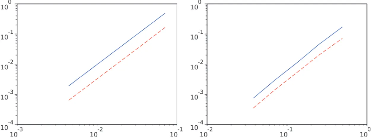
To verify numerically that the estimation of the error 𝑒ℎ,𝑘:= |𝜆𝑘− 𝜆ℎ,𝑘| is of order ℎ2as stated at the end
of Section 2.2, we shall consider a domain Ω where the exact eigenvalues are known and an exact boundary approximation is possible. Moreover, the eigenfunctions must be in 𝐻2(Ω), which is the case if Ω is convex as
mentioned in that subsection. A mesh refinement is then carried out: each triangle is divided into four similar triangles in order to have nested meshes with smaller and smaller parameter ℎ, so at each refinement, ℎ is halved.
In ℝ2we consider the square 𝑆 := [0, 1] × [0, 1]. A simple separation of variables shows that the spectrum
of 𝑆 is the set
{(𝑘2+ 𝑙2)𝜋2| 𝑙, 𝑘 ∈ ℕ \ {0}}.
The experimental error 𝑒ℎ,1obtained seems to verify the theoretical result mentioned previously [6, Theo-rem 3.1] (the slopes in Figure 1 are approximatively equal to 2).
On the sphere, no simple example with exact boundary approximation has been found. However, it is known that the first eigenvalue of −Δ𝑔on 𝕊2is 2 and that the coordinate functions in ℝ3are associated eigen-functions; see [8, Section II.4, Proposition 1]. In particular, they have a hemisphere as a nodal domain, and so the first eigenvalue of a hemisphere is also 2, that is,
𝜆1(𝐵𝜋/2(S)) = 2,
where 𝐵𝜋/2(S) is the ball centered in S = (0, 0, −1) of radius 𝜋/2 in 𝕊2, namely the southern hemisphere. Notice that the order of convergence in that case is the same, despite of the approximation of the domain. For both examples, the computed error 𝑒ℎ,1is represented in Table 1 and in Figure 1.
To illustrate the convergence of the optimization algorithm, we chose the seventh eigenvalue of a domain of volume 0.1 in the Poincaré disc. The motivation to present such an example comes from the need to take the metric into consideration to deal with it. Moreover, the associated optimizing domain is non-symmetric as presented in the sequel.
The method of optimization described in Section 3.1 is based on a descent algorithm, which provides
local minima. Starting from various initial domains is necessary to enhance the effectiveness of the method
to find global minima. In this article, only an example leading to the shape having the smallest eigenvalue obtained is given, namely a square. See [25] for a more complete presentation. Its boundary is discretized
ℎ 𝑒ℎ,1(𝑆) with (left) and
without (right) masslumping
ℎ 𝑒ℎ,1(𝐵𝜋/2(S)) with (left) and
without (right) masslumping
0.2√2/22 −0.164, 0.488 0.492 −0.072, 0.171
0.2√2/23 −0.041, 0.122 0.253 −0.020, 0.046
0.2√2/24 −0.010, 0.030 0.135 −0.006, 0.012
0.2√2/25 −0.003, 0.008 0.0706 −0.002, 0.003
0.2√2/26 −0.0006, 0.0019 0.0380 −0.0004, 0.0007
Table 1.Error resulting from the approximation of 𝜆1(𝑆) ≃ 19.739 on nested meshes of the square 𝑆 ⊂ ℝ2(left) and of 𝜆1(𝐵𝜋/2(S)) = 2 on nested meshes of the hemisphere 𝐵𝜋/2(S) ⊂ 𝕊2(right).
Figure 1.Graph of ℎ → 𝑒ℎ,1(𝑆) (left) and of ℎ → 𝑒ℎ,1(𝐵𝜋/2(S)) (right) in a logarithmic scale. The blue plain curves correspond to
computations without masslumping and the red dashed ones to computations with masslumping.
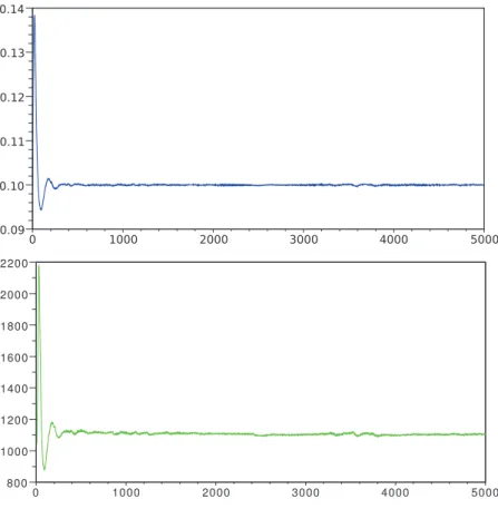
uniformly using 100 points corresponding to 1250 triangles. Then the optimization algorithm is performed and a candidate to be an optimal domain is obtained. To reach better accuracy, two successive refinements of the mesh are performed similar to those used in the first experiment described in this subsection. Figures 2 and 3 represent the evolution of the Lagrange multiplier during the optimization process, together with the evolution of the volume, the eigenvalue and the value of the cost functional 𝐽 introduced in Section 3.1. In this example, all these quantities converge relatively quickly, in particular the volume converges to the ini-tial volume as requested by the constraint imposed in the optimization problem. The value of the obtained eigenvalue 𝜆∗
7(Ω7,𝔻2) and the corresponding domain Ω7,𝔻2are given in Table 3.
4.3 Numerical Investigations
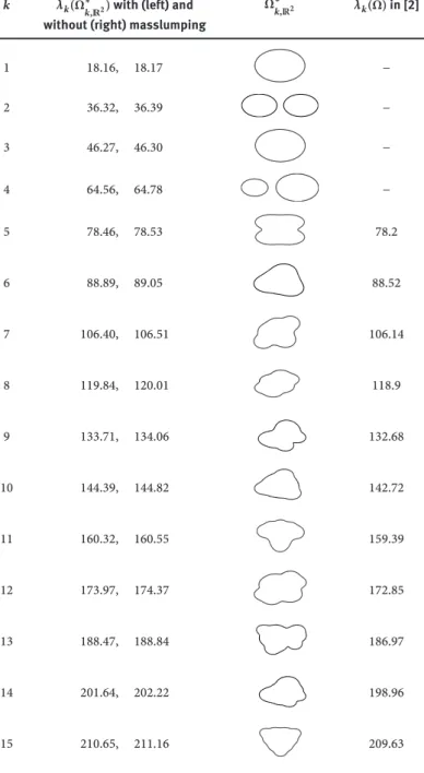
First, the program is run to find the optimizer Ω∗𝑘,ℝ2, 𝑘 = 1, . . . , 15, for the fifteen first eigenvalues in ℝ2.
Even if the volume constraint is not necessary in this case, the program is used without any modifications to compare the results with [2, p. 13]. The shapes obtained match the ones in [2]. They are presented in Table 2, each eigenvalue being computed with and without masslumping.
Remark 4.1. To reach the optimal domain, the program is started from various initial discretized boundaries.
In particular, they have different numbers of connected components. For 𝜆𝑘(Ω) with Ω ⊂ ℝ2and 𝑘 ≥ 2, it
happens that resulting domains are made of connected component realizing the optimum for 𝜆𝑙with 𝑙 < 𝑘. This is related to the result from Wolf and Keller [26, Theorem 8.1]. In spite of the lack of homothety in 𝕊2and
𝔻2, a similar behavior is noticed in these cases.
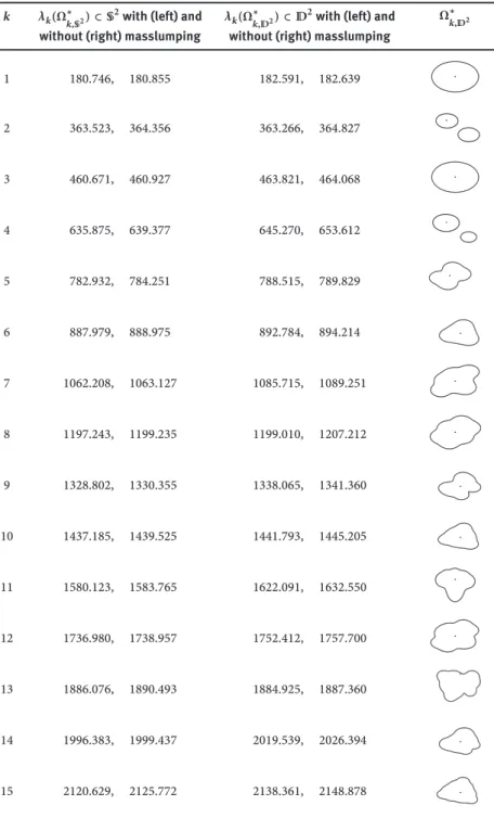
Another numerical experiment consists in computing the optimizers for small domains in the sphere and in the Poincaré disc. Let Ω∗
𝑘,𝕊2and Ω ∗
𝑘,𝔻2 denote the optimizer for the 𝑘-th eigenvalue in the sphere and in
Figure 2.Evolution of the volume of the domain (top) and of the cost functional L (bottom) with respect to the iteration of the
optimization process starting from Ω𝑠.
Figure 3.Evolution of the eigenvalue of the domain (top) and of the Lagrange multiplier (bottom) with respect to the iteration of
𝑘 𝜆𝑘(Ω∗𝑘,ℝ2) with (left) and without (right) masslumping
Ω∗ 𝑘,ℝ2 𝜆𝑘( ̃Ω) in [2] 1 18.16, 18.17 − 2 36.32, 36.39 − 3 46.27, 46.30 − 4 64.56, 64.78 − 5 78.46, 78.53 78.2 6 88.89, 89.05 88.52 7 106.40, 106.51 106.14 8 119.84, 120.01 118.9 9 133.71, 134.06 132.68 10 144.39, 144.82 142.72 11 160.32, 160.55 159.39 12 173.97, 174.37 172.85 13 188.47, 188.84 186.97 14 201.64, 202.22 198.96 15 210.65, 211.16 209.63
Table 2.Numerical approximation of 𝜆𝑘(Ω∗𝑘,ℝ2), 𝑘 = 1, . . . , 15, for Ω∗𝑘,ℝ2 ⊂ ℝ2the optimizer of volume 1 for the 𝑘-th eigenvalue and corresponding shapes. The last column contains the eigenvalues 𝜆𝑘( ̃Ω) from [2].
domains look like those found in ℝ2. Such computations have been made with a fixed volume 𝑉0 = 0.1; see Table 3. The domains in the Poincaré disc are also exhibited in this table. Visualizing domains in the sphere is not always convenient so only one example is shown here; see Figure 4. All these results confirm the above expectation.
Then the value of the volume 𝑉0has been increased up to 2 for domains in the sphere and in the Poincaré disc. The relation between vol(Ω∗
𝑘,𝕊2) and 𝜆𝑘(Ω∗𝑘,𝕊2) is exhibited in Figure 5.
Several remarks can be added to the results of these tables. Concerning the domains obtained having two connected components, namely the candidates for the optimizer of the second and the fourth eigenvalue, the ratio between the volume of the connected components has been performed for both in each space ℝ2, the sphere and the Poincaré disc. First for the plane: theoretically, the ratio for the second eigenvalue is 1 by the
𝑘 𝜆𝑘(Ω∗𝑘,𝕊2) ⊂ 𝕊2with (left) and without (right) masslumping
𝜆𝑘(Ω∗𝑘,𝔻2) ⊂ 𝔻2with (left) and without (right) masslumping
Ω∗ 𝑘,𝔻2 1 180.746, 180.855 182.591, 182.639 2 363.523, 364.356 363.266, 364.827 3 460.671, 460.927 463.821, 464.068 4 635.875, 639.377 645.270, 653.612 5 782.932, 784.251 788.515, 789.829 6 887.979, 888.975 892.784, 894.214 7 1062.208, 1063.127 1085.715, 1089.251 8 1197.243, 1199.235 1199.010, 1207.212 9 1328.802, 1330.355 1338.065, 1341.360 10 1437.185, 1439.525 1441.793, 1445.205 11 1580.123, 1583.765 1622.091, 1632.550 12 1736.980, 1738.957 1752.412, 1757.700 13 1886.076, 1890.493 1884.925, 1887.360 14 1996.383, 1999.437 2019.539, 2026.394 15 2120.629, 2125.772 2138.361, 2148.878
Table 3.Numerical approximation of 𝜆𝑘(Ω∗𝑘,𝑀), 𝑘 = 1, . . . , 15, for Ω∗𝑘,𝑀the optimizer of volume 0.1 in 𝑀 = 𝕊2and 𝔻2for the 𝑘-th
eigenvalue.
Krahn–Szegő theorem. Moreover, if the optimizer for the fourth eigenvalue is the union of two discs, as it seems to be numerically, the ratio is
𝑗20,1 𝑗2
1,1
≃ 0.394,
by [11]. Numerically, we found 0.390. Although no such results exist in 𝕊2and in the Poincaré disc, due to
the non-invariance by homothety of Ω → vol(Ω)𝜆𝑘(Ω) in these spaces, the corresponding ratios are given for comparison. In 𝕊2they are about 0.997 and 0.392, respectively, whereas for the Poincaré disc, they are about
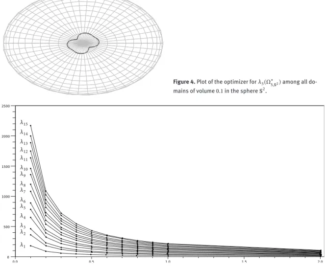
Figure 4.Plot of the optimizer for 𝜆5(Ω∗5,𝕊2) among all
do-mains of volume 0.1 in the sphere 𝕊2.
𝜆1 𝜆2 𝜆3 𝜆4 𝜆5 𝜆6 𝜆7 𝜆8 𝜆9 𝜆10 𝜆11 𝜆12 𝜆13 𝜆14 𝜆15
Figure 5.Plot of 𝜆𝑘(Ω∗𝑘,𝕊2) with respect to vol(Ω∗𝑘,𝕊2) for 𝑘 = 1, . . . , 15.
Besides, another remark is related to the evolution of 𝜆𝑘(Ω∗
𝑘,𝐸), 𝑘 = 1, . . . , 15, with respect to the volume of
Ω∗𝑘,𝑀for the three models 𝑀 = ℝ2, 𝕊2, 𝔻2. In the plane, this relation is of the form 𝜆𝑘(Ω∗𝑘,ℝ2) = cst𝑘/vol(Ω∗𝑘,ℝ2),
𝑘 = 1, . . . , 15, where cst𝑘is a positive constant, explicitly known for 𝑘 = 1 and 2 by the Faber–Krahn and the Krahn–Szegő theorems. The corresponding plots for 𝕊2are given in Figure 5. In each case, the shape of the optimizer does not change considerably for close volume, as illustrated in Figure 6, for 𝜆10(Ω∗
10,𝕊2). To
compare the three models, see Figure 7 which shows the evolution for the first two eigenvalues. Notice that these eigenvalues decrease less in the Poincaré disc than in ℝ2and in the sphere, where the slope is the
deepest.
Finally, some computations in the upper sheet 𝐻 of the hyperboloid have been performed. The Gaussian curvature of this model is given by
𝜅(𝑟, 𝜃) = 1 (1 + 2𝑟2)2.
In particular, the Gaussian curvature is non-constant, strictly positive and attains its maximum at the point (0, 0) with 𝜅(0, 0) = 1. Not surprisingly, numerical experiments show that the optimizer Ω∗1,𝐻for 𝜆1is a disc centered at (0, 0, 1). But, although the curvature lies between 0 and 1 in the hyperboloid, this eigenvalue is larger than the first eigenvalue of a ball of same volume in the plane (curvature 0), which is larger than the first eigenvalue of a ball of same volume in the sphere (curvature 1). For instance, denoting by 𝐵𝑀,0.01the ball of volume 0.01 in 𝑀, it yields numerically
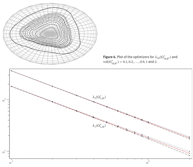
Figure 6.Plot of the optimizers for 𝜆10(Ω∗10,𝕊2) and
vol(Ω∗10,𝕊2) = 0.1, 0.2, . . . , 0.9, 1 and 2.
𝜆1(Ω∗1,𝑀)
𝜆2(Ω∗1,𝑀)
Figure 7.Plot of 𝜆𝑘(Ω∗𝑘,𝑀) with respect to vol(Ω∗𝑘,𝑀) for 𝑘 = 1, 2 and 𝑀 = ℝ2, 𝕊2, 𝔻2, in a logarithmic scale. The blue dotted curve, the red plain curve and the dashed black curve concern the Poincaré disc, ℝ2and the sphere respectively. The modulus
of the slope for the Poincaré disc is less than 1, whereas it is equal to 1 for ℝ2and it is larger than 1 for the sphere.
For the second eigenvalue, the obtained candidate Ω∗2,𝐻for the optimizer is two discs of same volume, tangent at the point (0, 0, 1). The eigenvalue computed is about 3643.50. So, as for the first eigenvalue, the same ranking with respect to the space occurs for the second eigenvalue.
Since the Gaussian curvature is radial and has its maximum at (0, 0), an optimizer Ω∗
𝑘,𝐻having its center
of mass at the origin is expected. The results found for the first two eigenvalues confirm this property. We focused also on the cases 𝑘 = 4 and 𝑘 = 13 since the corresponding optimizers found in the spaces previously studied are not symmetric. Numerically, for a volume equal to 0.1, the candidates for the optimizers are those expected (same shape as the corresponding domains found before) and their center of mass are at (0, 0, 1) (actually at a distance of about 10−9of this point); see Figure 8. Looking at the eigenvalues obtained, both 𝜆4(Ω∗4,𝐻) ≃ 658.329 and 𝜆13(Ω∗13,𝐻) ≃ 1905.911 are above the corresponding eigenvalues in ℝ2, in 𝕊2and in 𝔻2.
In conclusion, the algorithm presented in this article gives the same optimizers in ℝ2 as those found previously by the community, and permits to extend the study to other surfaces, even if they do not embed into ℝ3. It can thereby give an intuition in some cases not yet well known theoretically. Thus, some particularities arise quickly because few results exist, as the fact that the eigenvalues of the optimizers for domains in the hyperboloid lie above those in ℝ2and in 𝕊2.
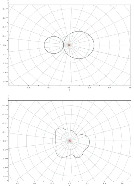
Figure 8.Plot of the optimizers Ω∗
4,𝐻for the fourth eigenvalue (above), and Ω∗13,𝐻for the thirteenth eigenvalue (below), among
all domains of volume 0.1. Their center of mass, indicated by a red cross, lie at the origin.
References
[1] G. Allaire, Conception Optimale de Structures, Math. Appl. (Berlin) 58, Springer, Berlin, 2007.
[2] P. R. S. Antunes and P. Freitas, Numerical optimization of low eigenvalues of the Dirichlet and Neumann Laplacians, J. Opt.
Theory Appl.154(2012), 235–257.
[3] P. R. S. Antunes, P. Freitas and J. B. Kennedy, Asymptotic behaviour and numerical approximation of optimal eigenvalues of the Robin Laplacian, ESAIM Control Optim. Calc. Var. 19 (2013), 438–459.
[4] M. G. Armentano and R. G. Durán, Mass-lumping or not mass-lumping for eigenvalue problems, Numer. Methods Partial
Differential Equations19(2003), 653–664.
[5] M. S. Ashbaugh and R. D. Benguria, Isoperimetric inequalities for eigenvalues of the Laplacian, in: Spectral Theory and
Mathematical Physics: A Festschrift in Honor of Barry Simon’s 60th Birthday, Proc. Sympos. Pure Math. 76, American
Mathematical Society, Providence (2007), 105–139.
[6] I. Babuška and J. E. Osborn, Estimates for the errors in eigenvalue and eigenvector approximation by Galerkin methods, with particular attention to the case of multiple eigenvalues, SIAM J. Numer. Anal. 24 (1987), 1249–1276.
[7] D. Bucur, Minimization of the 𝑘-th eigenvalue of the Dirichlet Laplacian, Arch. Ration. Mech. Anal. 206 (2012), 1073–1083. [8] I. Chavel, Eigenvalues in Riemannian Geometry, Pure Appl. Math. 115, Academic Press, Orlando, 1984.
[9] P. G. Ciarlet, The Finite Element Method for Elliptic Problems, Stud. Math. Appl. 4, North-Holland, Amsterdam, 1978. [10] P. G. Ciarlet, Introduction à l’analyse numérique matricielle et à l’optimisation, Collection Mathématiques Appliquées pour
la Maîtrise, Masson, Paris, 1982.
[11] B. Colbois and A. El Soufi, Extremal eigenvalues of the Laplacian on Euclidean domains and closed surfaces, preprint (2012), hal.archives-ouvertes.fr/docs/00/95/70/58/PS/Extremal-eigenvalues4.ps.
[12] R. Courant and D. Hilbert, Methods of Mathematical Physics, vol. I, Interscience Publishers, New York, 1953.
[13] A. El Soufi and S. Ilias, Domain deformations and eigenvalues of the Dirichlet Laplacian in a Riemannian manifold, Illinois
J. Math.51(2007), 645–666.
[14] M. S. Engelman, R. L. Sani and P. M. Gresho, The implementation of normal and/or tangential boundary conditions in finite element codes for incompressible fluid flow, Internat. J. Numer. Methods Fluids 2 (1982), 225–238.
[15] D. Gilbarg and N. S. Trudinger, Elliptic Partial Differential Equations of Second Order, Classics Math., Springer, Berlin, 2001. Reprint of the 1998 edition.
[16] P. Grisvard, Elliptic Problems in Nonsmooth Domains, Monogr. Stud. Math. 24, Pitman, Boston, 1985.
[17] P. Grisvard, Singularities in Boundary Value Problems, Recherches en Mathématiques Appliquées 22, Masson, Paris, 1992.
[18] A. Henrot, Extremum Problems for Eigenvalues of Elliptic Operators, Front. Math., Birkhäuser, Basel, 2006.
[19] M. Jumonji and H. Urakawa, The eigenvalue problems for the Laplacian on compact embedded surfaces and three dimen-sional bounded domains, Interdiscip. Inform. Sci. 14 (2008), 191–223.
[20] A. V. Knyazev and J. E. Osborn, New a priori FEM error estimates for eigenvalues, SIAM J. Numer. Anal. 43 (2006), 2647–2667.
[21] R. B. Lehoucq, D. C. Sorensen and C. Yang, ARPACK Users’ Guide, Software, Environments, and Tools 6, SIAM, Philadel-phia, 1998.
[22] D. Mazzoleni and A. Pratelli, Existence of minimizers for spectral problems, J. Math. Pures Appl. (9) 100 (2013), 433–453. [23] A. Munnier, Stabilité de liquides en apesanteur, régularité maximale de valeurs propres pour certaines classes
d’opérateurs, Ph.D. thesis, Université de Franche-Comté, 2000.
[24] É. Oudet, Numerical minimization of eigenmodes of a membrane with respect to the domain, ESAIM Control Optim. Calc.
Var.10(2004), 315–330.
[25] R. Straubhaar, Numerical optimization of Dirichlet–Laplace eigenvalues on domains in surfaces, Ph.D. thesis, University of Neuchâtel, 2013.
[26] S. A. Wolf and J. B. Keller, Range of the first two eigenvalues of the Laplacian, Proc. Roy. Soc. London Ser. A 447 (1994), 397–412.