Tests of the Kolmogorov-Smirnov type for exponential data with unknown scale, and related problems

Biometrika (1976), 63, 1, pp. 149-60 1 4 9 Printed in Great Britain

Tests of the

Kolmogorov-Smirnov type for exponential data

with unknown scale, and related problems

B Y BARRY H. MARGOLIN

Department of Statistics, Tale University, New Haven, Connecticut

AND WTLLI MAURER

Wirtschafts-Mathematik AG and Swiss Federal Institute of Technology, Zurich

SUMMABY

Let 3, /5+ and 3~ denote Kolmogorov-Smirnov type one-sample statistics to test good-ness of fit in the presence of unknown nuisance parameters; then the distributions of f), £+

and 3~ depend on the population sampled and the estimator used. Simulation has been the primary tool for studying these statistics. Recently, Durbin obtained the distributions of

D, D+ and D~ in terms of a Fourier transform for a wide class of underlying populations,

and produced explicit results for the exponential case. In this paper, the distribution func-tions of D, z/+ and D~ for the exponential case are derived from general results for order statistics, and computationally efficient approximations to these distribution functions are obtained. In the course of this derivation, Bonferroni inequalities of Kounias, and Sobel & Uppuluri are generalized. Certain problems of goodness-of-fit testing in the presence of nuisance parameters, whose solutions make use of existing tables, are also discussed. These problems include the Pareto, Rayleigh, power function, and uniform distributions.

Some hey words: Bonferroni inequality; Composite hypothesis; Dirichlet distribution; Distance statistic;

Goodness of fit; Kolrnogorov-Srnirnov testa; Nuisance parameter; Order statistic.

1. INTRODUCTION

A voluminous literature exists for tests of goodness of fit based on the sample distribution function, but, as Durbin (1973, p. 47) has commented, it is surprising how little theoretical work has been done on tests based on the sample distribution function when the population distribution function is postulated only up to a set of nuisance parameters. Few realistic goodness-of-fit problems involve a fully specified population distribution function; more typically, the form of the null hypothesis of interest in a goodness-of-fit problem is that, for

6 a vector,

Ho:F(x) = Fo(x;0) (6eQ),

that is, a composite rather than a simple hypothesis.

In this situation, it is tempting to replace the nuisance parameters in Fo (z; 6) by efficient

estimators $, and then to form test statistics based on Fo (x; 0) as if it were a fully specified

distribution function. Thus, one might construct tests for a random sample of size n based on the maximum deviation between the sample distribution function, say Fn(x), and

150 BABRY H. MABGOLIN AND W I L L I MATJBEE

F

(x; d), that is testa of the form: reject H^ if

(i) D

($) = sup \F

(x) -F

(x;0)\> C

,

(ii) D+ 0) = supfi^z)-F

(x;0)} > C+

, (1-1)

(iii) D-(0) = mv{F

(x;0)-F

(x)} > C£

.

The test statistics in (1-1) mirror the Kolmogorov (1933) statistic, although the sampling

distributions under H

are no longer distribution-free when F

(x; 6) is continuous, but depend

on both F

(x; 6) and the choice of estimator for 6. Nevertheless, the class of tests in (1-1)

retains certain attractive features that commend the Kolmogorov test when no nuisance

parameter is involved. First, it avoids arbitrarily discretizing the hypothesized distribution

function and transforming the sample observations to counts, a process that is troublesome

in small samples, but is required by the natural competitor to D

(0), the chi-squared

good-ness-of-fit test. Secondly, as Durbin (1975) has shown, the distribution functions of the

statistics in (1-1) can be obtained for certain F

(x; 0) and maximum likelihood estimation

of 6. Thirdly, simulation studies by Lilliefors (1967,1969) and Stephens (1974) support the

thesis that the tests in (1*1) will generally be more sensitive to departures from H

than is

the chi-squared test. Thus, the class of tests represented in (1 • 1) warrants farther exploration.

To date, research on the behaviour of the tests in (1-1) has proceeded along two lines.

Simulation has been the primary path followed. For example, Lilliefors (1967), via

simula-tion, has produced tables of critical values for test (i) in (1-1) for a normal distribution with

unknown mean and variance, together with estimation of these two nuisance parameters

by the corresponding sample mean and variance. Lilliefors (1969) has also studied via

simulation the case of an exponential distribution with unknown scale parameter estimated

by the sample mean. Both papers include brief power studies. Stephens (1974), also using

simulation, has investigated the cases Lilliefors studied, but under a wider variety of

alternative distributions for F(x). In an analytic direction, Durbin (1975) appears to be

the only author to date who has an exact, albeit complex, numerical method for evaluating

tail-area probabilities of D

($), Z)+ (/?) and D^ (0) for a wide class of cases; Durbin

demon-strates the computational feasibility of his technique by producing tables of exact critical

values of the statistics in (1-1) for the exponential case.

In this paper, the case of exponentiality is considered in detail. In § 2 this case is

formu-lated explicitly and distribution functions for the statistics in (1*1) are derived analytically

in closed form expressions. In § 3, for purposes of deriving computationally efficient

approxi-mations to these distribution functions, new Bonferroni inequalities are produced. These

new inequalities generalize earlier results of Kounias (1968) and Sobel & Uppuluri (1972).

In § 4, the Bonferroni inequalities of § 3 are used to determine critical values for the statistics

in (1-1); in the process, one obtains new insight into the behaviour of the corresponding

tests. Finally in § 5, attention is turned to a class of distributions F

(x; 6) for which existing

tables may be employed. These include the Pareto, Rayleigh, power function, and uniform

distributions.

Kolmogorov-Smirnov tests for exponential data with unknown scale 151

2. A N EXACT SOLUTION FOB THE EXPONENTIAL CASE

After observing a random sample Xlt...,Xn, one may wish to determine whether these

data are reasonably consistent with an assumption of exponentiality for the sampled population. Specifically, the hypothesis is:

H0:F0(z;d) = l-e-*l° (d>0,x>0). (2-1)

The alternative hypothesis is that HQ is not tenable. Were a specific alternative in mind, one presumably would employ a testing procedure tailored to that alternative.

Many tests of fit of the hypothesis in (2-1) exist; Shapiro & Wilk (1972) proposed an analysis of variance test for exponentiality and also referenced an extensive literature of other tests of fit for this case. Attention in this paper will focus on the sampling behaviour of the test statistic (i) in (1-1) for the hypothesis in (2-1) together with $ = (Xx + ...+ Xn)jn,

the maximum likelihood estimate of 6. This test statistic is (Lilliefors, 1969)

Dn($) = BUV\Fn(x)-{l-exp(-nxfZXi)}\. (2-2)

X

If Xft) < ... < X(n) denote the order statistics corresponding to the original sample, then

it can easily be verified that

Dn(6) = max {D+ ($), D~ ( % (2-3)

where

D+ (0) = m a x [ 1 - {1 - e x p ( - n X

/ S

X

)}],

D~{8) = m a x

[

{

l

_

^

^

l

L

From (2-3) and (2-4) it follows that, for 0 < y < 1,

pr{Z)

(0) < y) =

< y, D~ 0) < y)

= pr{^ - y < 1 -exp(-nZ

/S^Z

) < ^ ± +y; i = 1, ...,nj (2-5)

where log* (x) = log a; (x > 1), log* (a;) = n (x < 1).

J£Yi = XJI,X} (i = 1, ...,n), then 27^ = 1; from Wilks (1962, p. 179), one learns that

the joint distribution of 7lt ...,7n is Dirichlet Dn(l,..., 1), that is

t

) j , (2-6)

where I(S) is the indicator function for set S.

If ZQJ ^ ... ^ Z(n) denote the order statistics corresponding to the 7lt...,7n, then

and

rW )= l 0 ( 0 ^ 7 ^ . . . <7M) . (2-7)

152 BABBY H. MABGOLIN AND WILLI MAUBEB

As a consequence of the constraint on 7$,, . . . . F ^ , the following inequalities hold with probability one:

0 < I t t ) < l / ( n - » + l) (* = l , . . . , n - l ) ; 1/n *S 7(n) < 1.

I t then follows that (2-5) is equivalent to

pr {£„(£) < y) = pr{L(t,n,y) «S 7(<) ^ U(i,n,y); » = 1, ...,n}, (2-8)

where

L

i,n,y) =

i(n,n,y) = max ji.ilog^j), (2-9)

U(i,n,y) = ° ^

This attention to bounds will avoid computational problems later.

In principle, the probability in (2-8) could be obtained directly by integrating the prob-ability density in (2-7) over the interval in R* defined by the expressions in (2-8) and (2-9); the integration, however, is best done in a two-stage operation.

First,>define

for all values of (ru ...,rn). Then, because 0 < F ^ < ... < F(n), it follows that

...,Cn) (2-10)

for Ct = max{0,max(rlt ...,ri)}. Note that 0 < Cj < ... < On.

Secondly, it follows from (2-8) that pr{Dn((?) < y} =

-[F{U(l,n,y),L(2,n,y),...,L(n,n,y)} + ...

,y),...,U(n,n,y)}. (2-11)

Equation (2-11) is justified by an argument identical to that which justifies expressing the probability of an n-dimensional interval in terms of an n-dimensional distribution function (Wilts, 1962, p. 49).

An expression for F(CV ...,Gn) has been obtained by Maurer & Margolin (1976) as a

special case of results for distribution functions of subsets of order statistics, namely

I n+1 )-l n (0,-0,-1)! n a, ^ . . . S ( a « _ i — n - 1 O i - l

x fl ( ^ " V "

) !

- S C

{a

-a

_

)]

'

l{i C^-a^) < l), (2-12)

Kolmogorov—Smirnov tests for exponential data with unknown scale 153

The result in (2-12) can be restated more compactly as

{

n(F

>Ci) = n ! S ( - l )

-

S

[UrA l - S ^ , I £ O

r

< 1), (2-13)

where Sr denotes summation over all positive integers (rv •••,rm) suoh that SirJ = n.

Formula (2-13) can be derived from (2-12) essentially by deleting the terms with combi-natorial coefficients equal to zero. The proof will be omitted. Durbin (1976) obtained formula (2-13) via Fourier inversion; he observed that (2-13) yielded the distribution function of

D%(0) for the exponential case if one sets C< = L(i,n,a) (i = 1, ...,n). Upon combining the

expressions in (2-9), (2-10), (2-11) and (2-13), one arrives at a closed analytic expression for the distribution function of Dn ($).

The statistics i>+ ($) and D~ ($) were first studied by Durbin (1975); he proved that the two statistics are not identically distributed and tabulated their critical values. I t is worth noting that if the alternative to (2-1) is one-sided, then Z>+ ($) and D^ {6) are intuitively appealing test statistics. For alternatives that are one-sided, and for alternative test procedures, see Hollander & Proschan (1972).

The distribution in (2-6) arises in many other seemingly unrelated contexts (David, 1970, §5-4). Thus, for example, the statistics in (1-1) may be used to test whether data observed

are consistent with the hypothesis that the observations are distances between successive points dropped at random in the interval [0,1], as Durbin (1975) has indicated. Similarly, one is also able to test whether data observed are consistent with the hypothesis that the

Ylt...,Tn are distances between midpoints of successive arcs of equal length that have been

randomly placed on the perimeter of a circle of unit circumference.

In §4 computationally efficient approximations to the distribution function o£Dn($) will

be derived; these approximations are based on new Bonferroni inequalities to be presented in the next section.

3. IMPBOVBD BONFEBBONI BOUNDS FOB THE PBOBABUJTY OF A UNION

For a finite set of events {Av ...,An] associated with a probability space (D,^",P),

Kounias (1968) has proved that

pr(u

{-1 i <+i

which clearly improves on the simple Bonferroni upper bound of S pr (At). Following Sobel

& Uppuluri (1972), one can define the degree of a bound, such as that in (3-1), as the maxi-mum number of events in any intersection whose probability is needed to evaluate the bound; the bound in (3-1) is then of degree two. Sobel & Uppuluri produce upper bounds of even degree, and lower bounds of odd degree, that are clear improvements over the standard Bonferroni bounds of degree one less, for degrees at least 2, but their results apply only if the events are exchangeable. The theorem that follows generalizes their results to non-exchangeable events.

THEOREM 3-1. Let

S

= 2

154 BARRY H. MARGOLIN AND W L L U MAURER

similarly, for a fixed integer r such that 1 ^ r ^ n, set

i

Then, for any odd degree v (3 < v ^ n),

B ( (3-2)

a - l r \ < - l / and for any even degree v (2 ^ v < n),

pr ( U ^ ) < s N - l J - ^ . - m a x ^ . (3-3)

Proof. Let 24(w) be the indicator random variable of At. Here maxl/j^),...,/„(«)} is

the indicator random variable for Ax u • • • U An.

For a fixed integer r such that 1 ^ r < n, define

a

*M

= S

i+r+j

The claim is made that for all we Q and odd v such that 3 < v < n,

/,(<») 7,(4 (3-4)

a - l

To prove (3-4), one must consider three possible cases.

(i) First, if A(w0) = 0 for all i, then both the left-hand side and the right-hand side of

(3-4) are zero.

(ii) Secondly, if Ir(w0) = 0 and exactly n — t—1 other indicator variables are zero for

a) = o>o (t = 1,...,» — 1), then t indicator variables are one for w = (oQ, and the left-hand side

of (3-4) is

' = - x ( - i ) * r . (3-5)

a - l

(3-6) which is less than or equal to 1, the right-hand side of (3-4).

(iii) Thirdly, if Ir (a)0) = 1 and exactly t other indicator variables are one for w = wQ (t = 0,1, ...,n— 1), then n — t — 1 indicator variables are zero, and the left-hand side is

as is the right-hand side.

Thus (3-4) is proved. Taking expectations in (3-4), one proves that

' s ' t - l J - ^ . + S W ^ p r f l J A{). (3-7) a - l \ < - l /

Kolmogorov-Smirnov tests for exponential data with unknown scale 155

To prove (3-3), one first establishes the inequality

max{/

(*),...,/,»} < j?(-l)^T

-Ty (3-8)

a - l

for v even (2 ^ v < n). Again this can be done directly by considering the cases (i)-(iii) above and using (3-6).

The inequality in (3'8), in turn, proves that

^ s V l ) -

^ . - ^ . (3-9)

i-l I a-l

Equation (3-9) holds for all r, so that (3-3) is also established. Four comments concerning Theorem 3-1 are in order. (I) If v = 2, then (3-3) reduces to Kounias's result in (3-1).

(II) For exchangeable events, (3-2) and (3-3) reduce to the bounds of Sobel & Uppuluri (1972, equations (1-1), (1-2)).

(HI) Various other inequalities generalizing the results of Sobel & Uppuluri to non-exchangeable events, and generalizing the results of Kounias beyond v = 3, can be derived in a fashion similar to Theorem 3-1. Only one will be presented here.

(IV) Sobel & Uppuluri (1972, p. 1558) indicate that the 'simple-minded' replacement of

Pan\/{a!(n — a) 1} in their results by Sa for nonexchangeable events does not follow from their

work. Such replacement would yield an upper bound for v even, and a lower bound for v odd, of „_!

2 (-l)°-^a + (-l)"-i-S,. (3-10)

a-i n

Because n~1'LT^) — n-^-vS^, it follows by averaging the bounds in either (3-2) or (3-3) that

(3-10) is valid but is weaker than (3-2) and (3-3).

For reasons that will be clearer in § 4, one further generalization of Theorem 3-1 is needed. Consider any disjoint subsets Jv...,Jm with union (1,...,»), and with m < n; extend the

notation of Theorem 3-1 by letting

<$'*>= Spr (4^), ^ ^ S p r l i ^ i ) , ....

i+rt

for rkeJk(k = l,...,m) the second sum being for i < jeJk, i + rk #=_?. Then the following

theorem can be proved.

THEOBHM 3-2. For any odd degree v (3 < v < n),

' s ( - l ) - i - 8 f

+ S max^i' < p r ( u A

), (3-11)

pr(G

\ < - l

. p (3-12)

a-l k-lrteJt

Proof. A proof similar to that of Theorem 3-1 is easily constructed and will be omitted.

Note that Theorem 3-1 is the special case of Theorem 3-2 with m = 1. For the case v = 2, see Kounias (1968). Finally, for exchangeable events, (3-11) and (3-12) are weaker than

(3-2) and (3-3), respectively.

In § 4 these inequalities will be applied to the approximation of the distribution function

166 BARRY H. MARGOLIN AND W I L L I MAURER

4 . APPROXIMATIONS TO THB DISTBIBTJTION BTJNOnON OF Dn(&)

The key to approximating the distribution function of Dn{6) via the results of § 3 is the

recognition that (2-8) implies that

pr{Z)

($) > y} = pr [jjJRot Wi, », y), U(i, n, y)]}]. (4-1)

At = (Y(i)$[L(i,n,y), U(i,n,y)]), B{ = {7U) < L(i,n,y)}, B<+n = P«> > V(i,n,y)} (» = 1 n),

then Ai = Bt U Bi+n, Bt n Bi+n = <}> and (4-1) may be written as

U<) = pr{( U^,) U ( U ^

By the principle of inclusion-exclusion, an alternative expression can be derived for the tail area probability of Dn($):

i

, 4

) - . . . . (4-2)

Equation (4-2) together with the results of §3 then gives rise to various inequalities that may be used to approximate (4-2) to any desired degree of accuracy. Samples of size 3 to 10 were considered. Work was not carried beyond n = 10 because Durbin's (1975) Table 3 had been verified to be correct in all cases for n ^ 10, and there seemed little point in proceeding further, given that the feasibility of the approximation approach had been established.

The bounds programmed are specified in the footnote to Table 4-3.

I t is important to note that all the probabilities involved can be expressed simply and linearly in various terms of the form

where

lL{ij,n,y) (j = 1 a),

*i \U(i

n,y) (j = s + 1,...,«).

The terms in (4-3) may then be evaluated via (2-10) and (2-12), or more easily, via formula (4-5) of Maurer & Margolin (1976).

I t is instructive to examine in detail a representative example of the computations involved in these approximations to the distribution function of Dn(d);n = 7andy = 0-309

are chosen for this purpose, the y value being the 0-20 critical value reported by Lilliefors (1969).

The marginal behaviour of each order statistic is contained in Table 4-1.

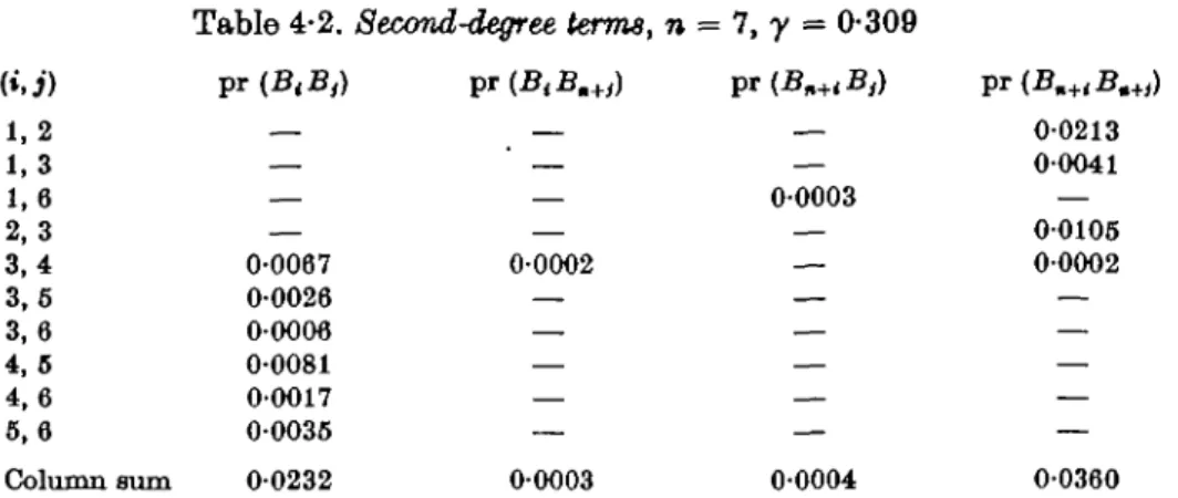
Table 4-2 contains the values of the second-degree terms, {pr (i^i^), ^T(BiBn+i),

pr (Bn+tBi), pr (Bn+iBn+i)} that are greater than zero to four decimals; all omitted terms

and terms replaced by a dash are zero to four decimals. Double precision accuracy was Table 4-1. prf-B,) and pr (Bi+n), n = 7, y = 0-309

Tail probabilities Tw < L(i, 7, 0-309)} F( 0 > U{%, 7, 0-309)} 0-0000 0628 0 0 •0000 •0666 00196 00373 0-0295 0060 0 0 •0235 •0000 0 0 •0108 •0000 00000 00000

Kolmogorov-Smimov tests for exponential data with unknown scale 157

T a b l e 4-2. Second-degree terms, n = 7,y = 0-309

(i,j) pr (BtB,) pi(BtBn+i) pr (Bn+(B,) pr(B.+ JB.+ j) 1,2 1,3 1,6 2 , 3 3,4 3,5 3,6 4 , 5 4 , 6 5,6 Column Bum — — — — 0-0067 0-0026 0-0006 00081 00017 00035 00232 — — 00213 — — 0-0041 — 00003 — — — 00105 0-0002 — 0-0002 00003 00004 0-0360

maintained, however, in all later computations, including the column sums. Two points concerning Table 4-2 are noteworthy. First,

S pr (£«£,+,), S VHB^iB,)

i<«/<7 i<«*<;7

are both negligible; since

pr {D+ (6) > y, Dj ($) > y} < £ {pr (BtB1+i) + pr (B^B,)},

the evente {Df 0) > y}, {Df 0) ^ y} are nearly exclusive. I n all cases examined, near exclusivity was found; this is consistent with the behaviour of the usual Kolmogorov statistics reported by Vandewiele & Noe" (1967), namely,

pr(Z>+ ^ y,D~ > y) < pr(Z)+ > y)pr(2)» ^ y).

Secondly, for fixed », both pr (BiBk) and pr (B7+iB7+k), for k + », 1 < k < 7 and 1 < t ^ 7,

decrease monotonically either as k takes the values % +1,..., 7, or as A takes the values t - l , . . . , l .

Third-order terms have not been given to save space. Based on these computations and others for y = 0-310, one finds the results in Table 4-3. Thus, the tail area probability for y = 0-310 is closer to 0-20 than is the tail area probability for y = 0-309; to be sure, the difference is negligible for all intents and purposes, but y = 0-310 is, to three decimals, the value obtained by Durbin (1975).

When » = 7 and y = 0-310, it was determined that, to three decimal places, pr{Z)+(0) >y} = 0-137, pr{Z>-(0) > y) = 0-063;

in all cases studied it was observed that pr{D+(#) Ss y} > pr{D~(#) ^ y}. This marked asymmetry, also evident in Table 4-1, is to be contrasted with the known symmetry in the behaviour of the usual Kolmogorov statistic. I t is precisely this asymmetry that is exploited by the bounds in Theorem 3-2.

Table 4-1 also illustrates another feature of the test, namely that

prfTo) < 2,(1,7, 0-309)} = 0, pr{7(7) ^ 17(7, 7,0-309)} = 0.

In Durbin's (1975) Table 3 one sees that y > vr1 for all critical values of interest; this

implies that U(n,n,y) = 1 and L(l,n,y) = 0. Therefore, if y > n"1, then

158 B A E B Y H . MARGOLIN AND WTT.TT MATJBEB

Statement (4-4) will be true for this test irrespective of the true model. The test as constructed should then exhibit insufficient sensitivity to the behaviour of the extreme order statistics when the alternative hypothesis is true.

Table 4-3. Probability bounds for pr{Z>7(0) ^ y}

7 (i) (ii) (iii) (iv) (v) (vi) (vii)

0-309 0-2562 0-2243 0-2079 0-2030 0-2025 0-2017 0-1963 0-310 0-2514 0-2204 0-2044 0-1996 01992 01984 0-1932 The bounds are: (i) standard Bonferroni upper bound, degree 1; (ii) Theorem 3-1 upper bound, degree 2; (iii) Theorem 3-2 upper bound, degree 2, m = 2, J1 = {1, .... n}, J , = {n+ 1, .... 2n}; (iv)

standard Bonferroni upper bound, degree 3; (v) Theorem 3-2 lower bound, degree 3, m, Jv Jt as

in (iii); (vi) Theorem 3-1 lower bound, degree 3; (vii) standard Bonferroni lower bound, degree 2.

Certain modifications of the test may counterbalance the insensitivity and asymmetry noted. A simple modification, for example, is the introduction of a weighting function, in the same spirit that Renyi (1953) and others have proposed weighting functions for the standard Kolmogorov statistic. Consider the general class of tests that follows:

Reject the hypothesis of exponentiality if

Wn (8) = max {W+ (8), W~ (8)} > Oan, (4-5)

where

W+ (8) = max (to}\± {1 exp (

-l«<n\ ln W~(8) =

K«nL

and {wf}, {«T} aie sstfl of specified weights; Durbin (1975) has also briefly discussed this

class of tests.

Tests of the class in (4-5) require evaluation of an expression of the form pr(a< < r( i )< 6<; t = 1,...,»),

which can be evaluated exactly by the method of Durbin (1975) and can be approximated by the bounds of the present section. One possible set of weights that will give greater import to the extreme order statistics is wf = wj = {i(n — i +1)/(« + I)2}"1. A more extreme set of

weights, taking all 10+ and w~ to be zero except for w~ = 1, produces a test equivalent to Fisher's (1929) maximum harmonic test with critical region F(n) > knA, a test that is not

thought of as a global goodness-of-fit test for exponentiality, but rather as a test for slippage.

5. PROBLEMS FOB WHICH EXISTING TABLES MAY BE EMPLOYED

The tables produced by Durbin (1976) for the exponential goodness-of-fit test under discussion have wider applicability than has been indicated previously. The following lemma extends the applicability in one direction.

LEMMA 5-1. IfXv ..., Xn are a random sample from a population whose distribution function Fx{x;6) has a maximum likelihood estimate 8(X), and ifYt = g(Xi) (i = 1,....«), where g is a monotonic transformation involving no parameters with inverse g-1, then the value of the statistic D* {8( Y)} in (1 • 1) based on Ylt..., 7n together with maximum likelihood estimation for

Kolmogorov-Smirnov tests for exponential data with unknown scale 159

Proof. We have

D*{$(7)} = max

I t suffices then and is easy to show that for all i, FY(Y(i), 6) equals Fx (X^y, 6) if g is

mono-tone increasing, and equals 1 — Fx(X^n_i+^;6) if g is monotone decreasing. This, together

with the fact that $( Y) = B(X) under the conditions of the theorem, yields the desired result.

The invariance in Lemma 5-1 extends to many statistics based on FX{X({),8(X)}, suoh

as the various goodness-of-fit test statistics considered by Stephens (1974).

Some examples of the use of Lemma 5-1 to extend the applicability of Durbin's table (1975) follow; all involve testing for goodness of fit via (1-1) together with maximum likeli-hood estimation for 6:

(i) Power function distribution, 6 > O:fr(y) = 0 - y i - W for 0 < y ^ 1. Here X = g~x{Y)

= —log Y has the distribution function in (2-1).

(ii) Pareto distribution, 0>O:fr(y) = 0-iy-w+ui<> f o r p l . Here, X = gr^Y) = log Y

has the distribution function in (2-1).

(iii) Rayleigh distribution, 6 > O:fY(y) = 2yd-1e^l'la for 0 < y. Here, X = g~HY) = Y1

has the distribution function in (2-1).

Similarly, a table of the distribution of the test statistic in (1-1) for the two-parameter normal model together with maximum likelihood estimation (Lilliefors, 1967) may be used for the two-parameter log normal model with maximum likelihood estimation.

An extension of the usefulness of existing tables in another direction is indicated by the following lemma, which is stated without proof:

LEMMA 5-2. Let M(x) be a Borel-measurable function on the real line such that the integral

exists for — ao<dx<62<co. The null hypothesis of interest is

(0 (x < 0X),

' {M(x)IN(0x,0i)}dx (dx^x^d2), (5-1)

(x

>

e

).

Consider a goodness-of-fit statistic to test (5-1) based on a random sample Xx,...,Xn (n > 3) of the form:

2 < « n - l

where (6X, £2) are maximum likelihood estimates. Then under Ho, the distribution of @n{Qx, $2) is identical to the distribution of Dn_z, the standard Eolmogorov statistic based on a sample of size n — 2 from a population with fully specified distribution function.

160 B A R R Y H . M A R G O L I N A N D WTT.T.T MATJRER

As an example, one could employ this result in testing goodness of fit of the uniform distribution U[dv 0 J . Note also that for the case of only one truncation point, the statistic

in (5-2) would be altered in an obvious way; @n(Q) would then be distributed as Dn_±.

Finally, although §5 has focused on extending the applicability of the table for Dn($),

analogous results could have been stated for the one-sided statistics £>+ (d) and Dn ($). The work was supported by U.S. Army, Navy, Air Force and N.A.S.A. under a contract administered by the Office of Naval Research, and by the Swiss National Foundation.

R E F E R E N C E S

DAVID, F. N. & JOHNSON, N. L. (1948). The probability integral transformation when parameters are estimated from the sample. Biometrika 35, 182-90.

DAVID, H. A. (1970). Order Statistics. New York: Wiley.

DUBBIN, J . (1973). Distribution Theory for Tests Based on the Sample Distribution Function. Phila-delphia: S.I.A.M.

DOBBIN, J. (1975). Kolmogorov-Smirnov tests when parameters are estimated with applications to testa of exponentiality and tests on spacings. Biometrika 62, 6-22.

FISHKB, R. A. (1929). Tests of significance in harmonio analysis. Proc. R. Soc. A 125, 54-9.

HOLLANDER, M. & PBOSOHAN, F. (1972). Testing whether new is better than used. Ann. Math. Statist. 43, 1136-^6.

KOLMOGOBOV, A. (1933). Sulla determinazione empirica di una legga di difltribuzione. Oiorn. 1st. Jtal.

Attuari 4, 83-91.

KOTTNIAS, E. G. (1968). Bounds for the probability of a union of events, with applications. Ann. Math.

Statist. 39, 2154-8.

LUXIEFOBS, H. W. (1967). On the Kolmogorov-Smirnov testa for normality with mean and variance unknown. J. Am. Statist. Assoc. 62, 399-402.

LrmKB'OBS, H. W. (1969). On the Kohnogorov-Smimov testa for the exponential distribution with mean unknown. J. Am. Statist. Assoc. 64, 387-9.

MAUBEB, W. & MABGOLTN, B. H. (1976). The multivariate inclusion-exclusion formula and order statistics from dependent variates. Ann. Statist. 4. To appear.

RENYI, A. (1953). On the theory of order statistics. Ada Math. Hung. 4, 191-231.

SHAPIBO, S. S. & WJXK, M. B. (1972). An analysis of variance test for the exponential distribution (complete samples). Technometrics 14, 355-70.

SOBEX, M. & UPFULUBI, V. R. R. (1972). On Bonferroni-type inequalities of the same degree for the probability of unions and intersections. Ann. Math. Statist. 43, 1549-58

STEPHENS, M. A. (1974). EDF statistics for goodness of fit and some comparisons. J. Am. Statist. Assoc. 69, 730-7.

VANDEWIELE, G. & NOB, M. (1967). An inequality concerning tests of fit of the Kolmogorov-Smirnov type. Ann. Math. Statist. 38, 1240-4.

WILES, 8. S. (1962). Mathematical Statistics. New York: Wiley.