Construction of a machine vision system for autonomous applications

CONSTRUCTION OF A MACHINE VISION

SYSTEM FOR AUTONOMOUS

APPLICATIONS

by

Anthony Nicholas Lorusso

Submitted to the

Department of Electrical Engineering and Computer Science

in Partial Fulfillment of the Requirements

for the Degree of

Master of Electrical Engineering

at the

Massachusetts Institute of Technology

May, 1996

(c) Anthonv Nieholas Loruss& 1996

Signature of Author

Depa

puter Science

May 23, 1996

Certified by

sermnold Klaus Paul Horn

Thesis Supervisor

Certified b

David S. Kang

Project Supervisor

Accepted bŽ

F. R. Morganthaler

Chair, Department Commitfee on Graduate Students

OF "TECiHNLOGY

1

JUN

111996

CONSTRUCTION OF A MACHINE VISION

SYSTEM FOR AUTONOMOUS

APPLICATIONS

by

Anthony Nicholas Lorusso

Submitted to the Department of Electrical Engineering and

Computer Science on May 23, 1996 in partial fulfillment of the

requirements for the Degree of Master of Electrical Engineering.

Abstract

The Vision System is a completed prototype that generates

navigation and obstacle avoidance information for the autonomous

vehicle it is mounted upon. The navigational information consists

of translation in three axes and rotation around these same axes

constituting six degrees of freedom. The obstacle information is

contained in a depth map and is produced as a by-product of the

navigation generation algorithm. The coarse prototype generates

data that is accurate to within 15%. The design methodology and

construction of the prototype is carefully outlined. All of the

schematics and code are included within the thesis.

Assignment of Copyright to Draper Laboratory

This thesis was supported by The Charles Stark Draper

Laboratory, Inc. through the Intelligent Unmanned Vehicle Center

(IUVC). Publication of this thesis does not constitute approval by

The Charles Stark Draper Laboratory, Inc. of the findings or

conclusions contained herein. It is published for the exchange and

stimulation of ideas.

I hereby assign my copyright of this thesis to The

Draper Laboratory, Inc., Cambridge, Massachusetts.

Charles Stark

/ pnthýt Nicholas

Lorusso

Permission is hereby granted by The Charles Stark Draper

Laboratory, Inc. to the Massachusetts Institute of Technology to

reproduce part and/or all of this thesis.

Acknowledgments

I would like to thank

Matthew Fredette, James Guilfoy, Berthold Horn, Anne Hunter,

William Kaliardos, David Kang, Dolores Lorusso, Grace Lorusso,

Donald Lorusso Sr., Stephen Lynn, Eric Malafeew, William Peake,

Ely Wilson.

Dedication

This thesis is dedicated to the people whom have made all of the

wonderful things in my life possible.

To my wife,

Dolores Marie Lorusso

my father in law,

Anthony George Sauca

and

Table of Contents

Introduction

15

1 The Theory Behind the System

17

1.1

The Coordinate System

17

1.2 The Longuet Higgins and Pradzny Equations

18

1.3 The Pattern Matching Algorithm

24

1.4 Motion Parameter Calculation Algorithm

27

1.5 Updating the Depth Map

32

1.6 Chapter Summary

33

2 Prototype Vision System Architecture

37

2.1 Natural Image Processing Flow

37

2.2 Environment Imager

38

2.3 Image Storage Module

40

2.4 Preprocessing Module

42

2.5 Pattern Matching Module

43

2.6 Postprocessing Module

44

2.7 User Interface

45

2.8 The Prototype Vision System Architecture

46

2.9 Chapter Summary

47

3

The Prototype Vision System Hardware

49

3.1

The Prototype Hardware

50

3.2 CCD Camera

51

3.3 Auto Iris Lens

53

3.4 Frame Grabber with Memory

55

3.5 PC104 Computer

57

3.6 The Pattern Matching Module

59

3.6.1 The Motion Estimation Processor 60 3.6.2 Addressing and Decoding Logic 61

3.6.3 Latches and Drivers 64

3.6.4 Control Logic 65

4 The Prototype Vision System Software

4.1 The Overall System Process

69

4.2 Flow Field Generation

70

4.2.1 Frame Grabber Control 72

4.2.2 Patten Matching Module Control 75

4.2.3 Flow Field Calculation 79

4.3 Motion Calculation

79

4.3.1 Motion Calculation Functions 80

4.4 Chapter Summary

83

5

Calibration, Results, and Performance

85

5.1

System Calibration

85

5.1.1 Scale Factors 85

5.1.2 Determining the Virtual Pixels 87

5.2 Initial Results

90

5.2.1 Initial Results Analysis 91

5.3 Average Vector Elimination Filter

92

5.4 Final Results

93

5.4.1

Final Results Analysis

94

5.5 Speedup

94

5.6 Chapter Summary

97

6 Conclusion

101

Appendix A Schematic of the Pattern Matching Hardware

105

Appendix B Complete Listing of the C Source Code

107

INTRODUCTION

The Vision System described within this thesis has been designed specifically for autonomous applications where an autonomous application is any system that can perform a function without assistance. A few good examples of autonomous systems are security robots, house alarms, or blind persons with seeing eye dogs -these particular examples would all benefit from the system described here.

The system is tailored for stereo or monocular camera arrangements, low power consumption, small packaging, and faster processing than any similar commercial Vision System available today. The ultimate goal of this thesis is to describe the construction of a complete vision that can be mounted on an autonomous vehicle. The prototype described here will serve as a "proof of concept" system for the new ideas introduced within it; the system can be considered as an iteration in a much larger process to produce a self contained vision processing unit, perhaps even a single application specific integrated circuit.

This thesis is the third in a series of documents produced by the Intelligent Unmanned Vehicle Center (IUVC) of The Charles Stark Draper Laboratory in Cambridge Massachusetts that focus on the topic of machine vision. The first document is "Using Stereoscopic Images to Reconstruct a Three -Dimensional Map of Martian or Lunar Terrain" by Brenda Krafft and Homer Pien. The second document is "A Motion Vision System for a Martian Micro-Rover" by Stephen William Lynn. The IUVC project was established in 1991 with the participation of undergraduate and graduate students from the Massachusetts Institute of Technology and other universities local to Boston.

IUVC has given birth to many autonomous robots and vehicles since its establishment. The first series of robots, the MITy's, were designed for Lunar and Mars exploration. IUVC's most notable microrover, MITy2, has a cameo appearance in the IMAX film "Destiny in Space." Currently IUVC is developing more sophisticated ground, aerial, and water crafts.

"Construction of a Machine Vision System for Autonomous Applications," builds very closely on IUVC's second vision system document, "A Motion Vision System for a Martian Micro-Rover."

The purpose of this paper is to clearly explain the prototype Vision System so that others, if desired, may be able to recreate it. Since, however, the paper will dwell heavily upon the work that was actually implemented in the Vision System only a few alternate solutions will be discussed.

As you will see, the Vision System described here is simple, novel, flexible, expandable, and fast.

CHAPTER ONE

THE THEORY BEHIND THE SYSTEM

This chapter will provide all of the background theory necessary to understand how the vision system works. The natural progression of the chapter is to build the mathematical models and equations in the context that they will be used.

The chapter starts by defining the coordinate system that will be used, followed by a derivation of the Longuet Higgins & Pradzny Equations. The rest of the chapter describes the pattern matching and motion calculation algorithms in conjunction with their supporting formulas. The supporting formulas include the Least Squares derivation for calculating motion parameters , the optimized depth formula for updating the depth map.

The Coordinate System

P (OBJECT

OPTICAL A)

'ER OF

JECTION

Figure 1. 1 The Coordinate System

The coordinate system defined here is not nearly as complicated as it appears. The origin is renamed the Center of Projection, since any ray of light coming from an object passes through it. All points that are on objects seen by our system are generally labeled P. Conversely all object points correspond to a unique image point on the Image Plane. An

image point is where the ray connecting an object point to the Center of Projection intersects the Image Plane; these are denoted by a lower case script p. The Z-axis is called the Optical Axis, and the distance along the Optical Axis between the Image Plane and the Center of Projection is the Principal Distance. Any motion of our coordinate system, along the axes is described by a translation vector t. The right handed angles of rotation along each of the axes are A, for the X-axis, B, for the Y-axis, and C for the Optical Axis.

Derivation of the Longuet Higgins & Pradzny Equations

An easy way to picture the coordinates is as though the Charge Coupled Device (CCD) Camera is permanently mounted at the Center of Projection, and that the Image Plane is the camera's internal CCD sensor. (See Figure 1.2).

Y OPTICAL 01 Z AXIS CK AND ITE CCD IERA 'D ARRAY/ AGE

Figure 1.2 CCD Camera Placement

The Optical Axis goes through the center of the camera and points out of the camera lens; this is the exact way that the coordinate system and camera will be used. Note that throughout this chapter, lowercase x & y refer to coordinates on the Image Plane.

A camera cycle is simple; an image from the camera is stored, the camera is moved, and a second image from the camera is also stored. The camera motion between images can be described in translation and rotation vectors. It is a nice twist to note that if the environment moved instead of the camera, it can still be described in the same way

with just a change of sign. The structures we will use to describe motions in our coordinate system are,

The translation vector,

t=[U V

w]

Equation 1.1 Translation Vector

where U, is translation in the X-axis, V is translation in the Y-axis, and W is translation in the Optical, or Z-axis. The rotation vector,

r = [A

B

Cf

Equation 1.2 Rotation Vector

where A, is the rotation in radians around the X-axis, B is the rotation around the Y-axis, and C is the rotation around the Optical, or Z-axis. It is importnat to note that in practice we will expect these values to be small angular increments.

In Equation 1.2 each of the rotations may be represented by rotation matrices [1]. The matrices for the rotations are in bold or have a subscriptm.

For angle A, rotation in the Y-Z plane,

1

0

0

A, = 0

cos A

sin A

0

- sin A

cos

A

Equation 1.3 Rotation Matrix for X-axis

cos

B

Bm=

0

sin B

- sin B

0

cosB

Equation 1.4 Rotation Matrix for Y-axis

For angle C, rotation in the X-Y plane,

Cm

sin C

cosC

0

0

0

1i

Equation 1.5 Rotation Matrix for Z-axis

An object point in the scene being imaged is described by coordinates in X, Y, Z,

P = [X Y zf

Equation 1.6 Object Point Vector

Camera motion causes an object point to appear in a new location. The new location is given by,

X

X

X

Y

Y

->t¢

Y[

Equation 1.7

where R is the multiplication multiplication the R matrix is,

= i

RY

-Vi

=RY

z

New Object Coordinate Equation

of equations 1.5, 1.4, and 1.3 respectively. After

R=

sinAsinBcosC+ cosAsinC -cosAsinBcosC+ sinAsin C

-sinAsinBsinC+ cosAcosC cosAsinBcosC+ sinAcosC

-sinAcosB

cosAcosB

Equation 1.8 The Complete Rotation Matrix

The order of multiplication of the rotation matrices is very important. In an attempt to backward calculate for C, B, and A the order of multiplication would have to be known. The rotation matrices have another concern in addition to their order of multiplication, the matrices have non-linear elements.

The ability to make the elements of the rotation matrices linear will allow them to be solved for easier. The best way to do this is to use a Taylor expansion to simplify our equations. Recall the Taylor expansion is,

(x - a)2

f

(x)=

f

(a)+ (x -

a)f

(a) +

f

"(a)+

2!

_f

f(")(a) +...

3!

n!

Equation 1.9 Taylor Expansion [2]

We will choose our expansion point to be P=(A=O, B=O, C=O), and our second-order terms are negligible. Thus, the Taylor expansion is,

dR .

dR

1R?

R=I+

Am+

Bmn+

C

n

where the partial derivatives are,

0 cosAsinBcosC-sinAsinC sinAsinBcosC+cosAsinC

1

°= 0 -cosAsinBsinC-sinAcosC -sinAsinBsinC+cosAcosC

L

-cos AcosB

-sinAcosB

-sinBcosC sinAcosBcosC -cosAcosBcos C

-=

_{sinBsinC -sinAcosBsinC}

_-cosAcoBsinC

cosB

sin AsinB

-cosAsinB

-cosBsin C -sinAsinBsinC+cos AcosC cosAsinBsinC+sinAcosC

-•

-cosBcosC -sinAsinBcosC-cosAsinC cosAsinBcosC-sinAsinC

0

0

0

and the partial derivatives evaluated at P are conveniently,

A

--1

01

_oJO

ii,

1

and so our Taylor expansion to the first order is,

0

0

0

+

-A

₀

-B

[0

0

+ -C

0

0

-Equation 1.11 Taylor Expansion to the First Order of R

Keep in mind that our coordinate system is perspective projection. To obtain Image Plane coordinates, x & y, normalized by the camera lens focal length, f, we take our world coordinates X & Y, and divide by the principal distance, which is Z:

x X

f

z

f

z

22

-1

0

R=I+ 0

0

0

01

-Finally, we can express our Image Plane motion field in terms of the indicated parameters. The motion field is made up of the motion of points in the Image Plane as the camera is translated and rotated. The components of the motion vector for a point in the Image plane are [3],

u

X

Z

f

v

-

Y Z

7

=y=

Y

f

Z

Z

Equations 1.12 Motion Field Equations

where the dotted quantities are functions of images and u is motion along the image plane x-axis, and v is motion along the image plane y-axis. Equations 1.12 were derived by the product rule of the normalized coordinate equations.

Now if we step back and examine the X, Y, Z world coordinates it is obvious that we can represent their dotted quantities or changes with respect to images as a difference,

X

X

X

X

U

Y

Y

-

Y

=(R-I)Y -V

Z

Z'

Z

Z

W

Equation 1.13 Dotted World Coordinates

Now, plugging the Taylor approximation into Equations 1.12 and simplifying, we get,

u

CY - BZ - U

f

Zz

v

AZ

-CX

-V

f

Z

X(BX

-

AY -W)

Z

Y(BX

-

AY-W)

Z

which simplify to the Longuet Higgins & Pradzny Equations,

u

f

xyA

x

yC

=

+

+1 B+

f

f

Z

f

_j

_f

Equations 1. 14 Longuet Higgins & Pradzny Equations [4]

OED

The Longuet Higgins & Pradzny equations provide a practical and clear relation between the components of the motion field in the Image Plane of a camera and the actual motion of the surrounding environment.

The Pattern Matching Algorithm

The camera cycle compares two consecutive CCD images using the pattern matching algorithm. The pattern matching algorithm produces the relative motion field that can be used to determine camera motion or gather information about obstacles in the environment, depending upon the need of the end user.

The information collected from the black and white CCD camera is stored in an nxm matrix of 8 bit values, where n is the horizontal resolution of the Image Plane and m is the vertical resolution of the Image Plane. The resolution of the Image Plane depends upon the number of pixels in the CCD of the camera used to image the environment. Each complete nxm matrix of the Image Plane is called a frame. Each 8-bit value, called a pixel, is the brightness of a particular point in the Image Plane. The range of brightness values varies between 0 and 255, with 0 being a black pixel and 255 being a white pixel. Together, all the pixels make up an image of the surrounding environment. (See Figure

A PIXEL IN THE CCD IMAGE PLANE. OPTICAL/Z AXIS

II!

Figure 1.3 The CCD Image Plane and Frame

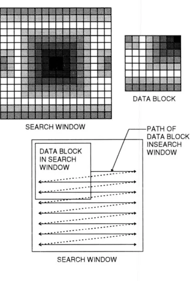
The operation of the pattern matching algorithm is functionally straight forward. The first frame is separated into data blocks nxn pixels in size. The second frame is separated into search windows 2nx2n pixels in size. The frame to block parsing is done such that there are the same number of data blocks and search windows. All of the data blocks have their centers at the same positions as the centers of the search windows in their respective frames. (See Figure 1.4).

FIRST AND SECOND DATA BLOCKS. NOTE THAT THE EDGE OF THE FIRST FRAME IS UNUSED. DATA BLOCK POSITIONS IN FIRST FRAME FIRST FRAME

FIRST AND SECOND DATA BLOCK POSITIONED IN FIRST AND SECOND SEARCH WINDOW

SECOND FRAME

Figure 1.4 First and Second Frames

The algorithm takes the first data block and finds its best match in the first search window. The best match position is then an offset from the data blocks original position. The offset is considered to be a measurement of the local motion field, where each of its components, u & v are the components of motion in Equations 1.14, the Longuet Higgins & Pradzny equations. Each offset will be called a flow vector.

25 I

1

I

-F

The best match is determined by the smallest error. A data block is initially placed in the upper left corner of its respective search window. The absolute value of the difference in the pixel values between the data block and search window are then summed to give the position error. The datablock is then moved to the right by one pixel and a new position error is computed. This process continues until the data block has been positioned at every possible location in its search window, See Figure 1.5. The data block location of the smallest position error is the desired value. If two position errors have the smallest value the second error computed is taken to be the best match. A description of the algorithm is,

n n n n

for(-

_{i <}

_-,

_-

_j

_<

_-):

2

2

2

2

n-1 n-1

PEi =

-

I

ISWx+i,y+J - DBx,,I

y=O x=O

if (PEi,

,

ME,,J)

then, ME = PEt=i,-=

Equation 1. 15 Pattern Matching Algorithm [5]

where PE is the position error, SW is the search window, DB is the data block, and ME is the minimum position error. The subscripts refer to specific locations in the respective data arrays. The value n is the width and height of a data block and, for hardware reasons discussed later, the upper left pixel in the search window is given the coordinate (n/2, -n/2). I & J are the position of the best match.

It is important to note that this algorithm does not provide us with any information

about the quality of the match. Further, the algorithm only provides integer pixel

resolution.

I

1

i

I

Figure 1.5 Movement of Data Block in Search Window

The position of the best match and its associated flow vector are calculated for each data block and search window pair. After all of the flow vectors have been calculated we have determined our complete motion field. It is important to note that the size of our search window places an upper bound on the magnitude of each flow vector. Hence, the amount of motion in a camera cycle is limited. It is also important to mention that we are assuming that the patterns in the frame parsed into data blocks are approximately the same patterns in the frame parsed into search windows; this is not a trivial assumption.

Motion Parameter Calculation Algorithm

The motion parameter calculation algorithm produces the final results of the vision system; It computes the 6 motion parameters described in Equations 1.1 and 1.2, and a depth map of the surrounding environment. The six motion parameters describe the net

:ii~~ _::~:j ~~~ _{:::~:i :::~ :~:~:~t~-:-:-:} " _::::::~j

I

i

I

~2.-

/

movement of the camera in a camera cycle. The depth map contains the estimated distances from the camera to large objects in the first frame of the camera cycle; a depth estimate is computed for each data block. Therefore, the resolution of the depth map is dependent on the size of the data block; the depth map can be thought of as the low pass filtered environment. The depth map suppresses all of the sharp detail and contrast an image can provide.

The motion algorithm simultaneously solves for the motion parameters and depth map; in a sense, they are by products of one another. The algorithm is an iterative process that assumes the correct motion parameters have been achieved when the depth map values converge. The motion algorithm is,

Figure 1.6 Motion Calculation Flow Chart

The first step in Figure 1.6 is to obtain the flow vector information from the pattern matching algorithm. A flow vector is formally defined as,

x',y' Matched Data Block Position

x,y Original Data Block Postion

and we can relate each flow vector to Equations 1.14, the Longuet Higgins & Pradzny equations by,

u=x=x'-x,

v=y=y'-y

Equations 1.16 Flow Vector Components

where the focal length has been set to one for convenience. The Longuet Higgins and Pradzny equations relate the motion field in the Image Plane to the actual motion of a

camera in our coordinate system, Figure 1.1. Since the pattern matching algorithm provides us with a means of determining the motion field in the Image Plane, it is sensible that we can solve for the six parameters of camera motion, U, V, W, A, B, C. We will define a vector m, that contains all of the motion parameters,

m=[U V

W

A

B

C]

Equation 1.17 Motion Parameter Vector

The motion parameter vector allows us to rewrite Equations 1.14, the Longuet Higgins & Pradzny equations, for each flow vector as,

O0

-

m

S~y

(y +1)

-xy

-x

L

Equation 1.18 Matrix Form of Longuet Higgins and Pradzny The matrix for all the flow vectors is calledA. A is a 2nxm matrix of the form,

-1

0

-1

Zn

0

-1

y_

(y2 +1)

(y( + 1)

-(x2 + 1)

-x

_y,

-(x + 1)

Yn

m = Am

Equation 1.19 Matrix of the Flow Vectors

Equation 1.19 is equal to the motion field derived from the pattern matching. Thus, an easy way of writing all the flow vectors in terms of the Longuet Higgins and Pradzny equations and setting them equal to the derived motion field is,

Am = [u,

Am=b

V, _{U2 V}

2

un

=

Equation 1.20 Flow Vectors Set Equal to the Motion Field

where b contains the components of the motion field derived from the pattern matching algorithm.

We still, however, need to find the best way to solve for m. If estimated values were chosen for m and A, an error could be defined between the b matrix containing the components of the motion field derived from pattern matching and the b matrix calculated from the estimated values of m & A. Since we have two parameters that the error could be optimized along, it is best to minimize the sum squared error. The sum squared error for a single flow vector is,

SSE =(U-u)

2

+ v )2

+(U

where u & v caret are derived from the Longuet Higgins and Pradzny equations. The error could be optimized to either the x-component, u, or the y-component, v. The total error for all the flow vector components in theb matrix would be

TSSE

(2

-

₎

_(n

_{- V.)}

n

Equation 1.22 Total Sum Squared Error for All Flow Vectors which can be also written, in matrix form, as,

IIAm-

b11

₌

₀

where,

Ix

12-=

x2

+X

X+...+x2

Equations 1.23 Matrix Form of Total Sum Squared Error

The equation Am=b is overdetermined as long as we use more than six flow vectors. The

beauty of the matrix form is that it can be shown to have the Least Squares solution form.

m = (ATA)-1A'b

Equation 1.24 Least Squares Motion Estimation Equation [6] Thus, we can solve for our motion given an estimated depth map.

Scale Factors

It is important to understand what the computed motion parameters and depth map mean. The rotations will always be in units of radians and the translations and depths will always be in the units of the principal distance, which are meters. The translations and depth values, however, will require scale factors to make them accurate. The easiest explanation for scaling is to observe that if the external world were twice as large and our velocity through the world were twice as fast all of our equations would generate the same flow field and depth map [7]. Unfortunately, determining the scale factor requires some knowledge of the environment external to the Vision System. Also, the scale factor can be

applied in two separate ways, either to the relative depth map or to the translation values themselves. Applying the scale factor to the translations requires measuring one of the parameters on axis and dividing by the estimated value to get the scale factor and then multiplying the other translations by it. Applying the scale factor to the depth map requires measuring the depth to a particular point in a scene and dividing it by the estimated depth value at that point to get the scale factor; this scale factor would then multiply all of the other depth values. Once we have either a corrected depth map or motion parameter vector we can calculate to get the correct motion parameter vector or depth map respectively.

Updating the Depth Map

Initially, we assumed the values of our depth map were constant; this allowed the first calculation of the motion parameters using Equation 1.24. A constant depth map, however, is not representative of a typical environment. To obtain more precise motion information a more accurate depth map may be needed. Hence, local correction of the depth map using the latest motion parameters could be done by isolating our unscaled depth Z, in terms of the six motion parameters and position. The equation for Z can be derived by optimizing the sum squared error between the motion field calculated by Equations 1.14, the Longuet Higgins and Pradzny equations, and the motion field computed from the pattern Matching. It is reassuring to note that this is the same sum squared error equation, Equation 1.21, that was used to derive the equation for the global motion parameters, Equation 1.24. The sum squared error with the full Longuet Higgins

and Pradzny equations inserted and the focal length set equal to one for simplicity are,

SSE

=

U

+xW)+xyA

-

IB+yC

uJ

((-V+yW) +(y2+1)A-xyB-xC_-v

to obtain a local minima we take the partial derivative with respect to Z, and set it equal to zero,

dSSE

(-U

+xW)2

dSSE

(-

Z

2+

(xyA

-_(X2+1)B

+ yC - ux-(-U

+xW))

+

dZ

z

(-

V+

_{_-}

_Z

yW))

22+

+ 1)A -xyB

-

xC

- v-(V

+ yW))

= 0

which, after some careful manipulation becomes our local depth Z,

(-U + xW)Y +(-V + yW)

(u-(xyA-(x2

1)B+yC))(-U+xW)+(V

+1)A-xyB-xC))(-V +yW)

Equation 1.25 Update Depth Map Equation [8]

Now, we use Equation 1.25, to update the depth map, where each flow vector has a single depth value. Heel has shown sufficient convergence of the depth map within ten iterations [9]. We will use convergence of the depth map as a measure of the reliability of the motion parameters calculated using it. It is only necessary to complete a full convergence cycle for the first computation of the motion estimates. The converged depth map can be used as the a priori depth map for the next motion estimate instead of a constant value. In most instances, this will decrease the number of iterations it takes the depth map to converge.

Chapter Summary

This chapter derived all of the pertinent Machine Vision equations necessary to understand this Vision System.

The chapter opened with a description of the coordinate system and data structures used within the chapter. The coordinate system is comprised of two components, the three dimensional world coordinate axes, and the two dimensional Image Plane. The world coordinate axes are labeled X, Y, Z, and the rotations are respectively,

A, B, C. The Image Plane coordinates are x, y. An object point, P, is in world coordinates

and described by Equation 1.6. An Image Point, p, is the contact location on the Image Plane of a ray that connects the Center of Projection, previously known as the origin of the world coordinate axes, and an object point. The Image Plane is actually the CCD of the camera used to view the environment. Any translation and rotation in the world coordinates is described as three dimensional vectors t & r, which are Equations 1.1 and Equations 1.2 respectively.

Immediately following the definitions of the coordinate system came the derivation of the Longuet Higgins and Pradzny equations, Equations 1.14. The Longuet Higgins and Pradzny equations provide a way of directly relating, within a scale factor, the motion field in the Image Plane to the six parameters of motion in world coordinates, where the motion field is a set flow vectors detailing how objects in the Image Plane move. A flow vector has two components, u & v which are change in x & y respectively.

Pattern Matching is used to measure the motion field between two consecutive frames. The frames are broken into manageable pieces that the pattern matching is performed on. Each small piece of the first frame is found in a corresponding larger piece of the second frame by finding the location of minimum error, called a best match. The size of the pieces that each frame is broken into determine the maximum value that a flow vector can be. The number of pieces that the frames are broken into determines the resolution of the Vision System. The Pattern Matching Algorithm is defined in Equation

1.15.

Following the pattern matching is the derivation of the equation that calculates the six motion. parameters, Equation 1.24. The equation takes two sets of numbers and computes the Least Squares values of the six motion parameters. The first set of numbers is a matrix A, calculated from the depth, Z, and the x, y positions of each flow vector. The second set of numbers is a matrix b, which contains all of the flow vector components determined from pattern matching. The six motion parameters U, V, W, A, B, C, are each elements of matrixm.

The cycle to calculate the six motion parameters is an iterative algorithm that assumes that the motion parameters are correct, to within a scale factor, when the depth map converges. The cycle takes a depth map, assumed constant only on the first cycle, and is delineated in Figure 1.6.

The chapter concludes with the derivation of the equation used to update the depth map, Equation 1.25. The equation performs local depth calculation using the six global

motion parameters in matrixm, and the original positions of each flow vector.

The chapter not only describes all of the major theory implemented within this Vision System, but provides a brief introduction into the field of Machine Vision; the field of vision has many more facets than those presented here.

CHAPTER TWO

PROTOTYPE VISION SYSTEM ARCHITECTURE

Chapter two presents the system architecture used in the prototype vision system developed for this thesis. The prototype serves as a proof of concept.

The chapter starts by outlining the natural way to perform image processing as described within this thesis. Each functional block of the natural image processing flow is considered and the important design issues are defined. The chapter concludes by presenting the architecture used in the prototype proof of concept system developed for this thesis.

The Natural Image Processing Flow

LIGHT

ENVIRONMENT

IMAGE

IMAGE

PATTERN MATCHING

IMAGER

STORAGE

DISTRIBUTION

MODULE

MOTION

USER

ESTIMATION INTERFACE OUTPUT

Figure 2. 1 Natural Image Processing Block Diagram [10]

The implementation of the theory developed in this thesis has a natural progression which can easily be represented as a block diagram, see Figure 2.1. The functional blocks

are the Environment Imager, Image Storage, Image Distribution, Pattern Matching, Motion Estimation, and a User Interface. The following sections describe each of the functional components and their primary design concerns.

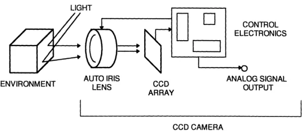
The Environment Imager

I If.I Ir I

L-UI

ONTROL CTRONICS

AUTO IRIS ANALOG SIGNAL

ENVIRONMENT _LENS LENS CCD OUTPUT_OUTPUT

ARRAY

CCD CAMERA

Figure 2.2 The Environment Imager

The environment imaging module is used to convert reflected light from the surroundings into usable information, see Figure 2.2. There are many techniques used to image an environment, however, the most common manner is to use a charge coupled device (CCD) camera.

A CCD camera uses a grid of photoelectric sensors that separate charge, and thus

create a voltage across them when exposed to certain frequencies of light. CCD arrays are typically made from silicon and thus have the typical spectral responsivity for a silicon detector. Each photoelectric element in a CCD array is called a pixel. The camera uses a lens that focuses the environment being imaged onto the CCD. A CCD controller then shifts the voltages from the CCD elements out. In order to make a CCD camera applicable to the current video standards, the digital data shifted out of the CCD is converted into one of the standard analog formats. Some of the analog formats are NTSC, CCIR/PAL. The number of pixels in the CCD array gives the resolution of the camera; it is usually best to get a camera with a large number of pixels (i.e. high resolution.)

CCD arrays come in many different styles depending upon the application. One

type of CCD array is for color cameras. A color camera has three separate analog signals; one for each of the colors red, green, blue. Although color CCD cameras can also be used

with this system, a black and white camera makes more practical sense since we are not trying to identify any objects or edges using colors, but by contrast. In a pattern matching system, a color camera requires three times as much processing as that of a black and white camera. We want to identify where different objects are and how they move. In a black and white camera colors are seen as shades of gray; this is advantageous when we make the constant pattern assumption since all of the contrast information is contained in each captured image.

The CCD array in a camera can also have pixels that are different shapes. Arrays can be purchased with hexagonal, circular, and square pixels. An array with circular pixels does not use all of the available light to generate its image data. CCD's with hexagonal pixels have a complicated geometry that must be considered when the data is processed. Therefore, the array with square pixels is the best possible choice for our application.

The CCD, however, is not our only concern about using a CCD camera as the environment imager. The amount of light that impinges on the CCD and contrast control are of equal importance.

The camera should have the ability to control the total amount of light that is focused on the CCD by opening and closing an iris; this feature is called auto iris. The auto iris controls the amount of light that enters a camera so that the full dynamic range of the CCD array can be used; it keeps the CCD from being under illuminated, or from being saturated by over illumination.

The last important feature of the environment imager is that the overall image contrast, gamma, should be able to be controlled. Many CCD cameras that are available allow the user to control gamma; this is especially important because Machine Vision may require higher contrast than the human eye finds comfortable.

The Image Storage Module

Figure 2.4 Block Diagram of the Image Storage Module

The frame storage module is used to convert the environment imaging signal into digital frame data and place it in a storage medium, see Figure 2.4. In our case, since we will be using a CCD camera to image the environment, it must convert an analog signal into digital pixel data that can be stored easily. The standard terminology for a device that converts camera output into pixel data is a "Frame Grabber."

As discussed in the Environment Imaging section, there are different video signal standards for the output of a CCD camera. Most often a Frame Grabber is designed to accept more than one video signal standard; a typical Frame Grabber will automatically adjust to the standard of the video signal connected to it.

Another important feature of some Frame Grabbers is the ability to store the pixel data it has created. The storage media can be of any type; some of the different types of media available are compact disc (CD), tape, hard disk, and non-volatile/ volatile Random Access Memory (RAM). The type of storage media dictates where the preprocessing module will have to look for the digital image information. The key factors in choosing the storage media are the amount of collected data, which is determined by the conversion rate of the Frame Grabber, and the ability to process the image data.

The conversion rate of a Frame Grabber, the speed that it can convert new analog signal data into digital pixel data, is called the "frame rate." The units of a frame rate are frames per second, which is the same units as the output of a CCD camera. The typical frame rate output for a CCD camera is 30 frames per second; this is actually predetermined by the video standard being used. It has been determined that at 30 frames

per second the human eye cannot detect the discreet change between any pair of frames.

The Frame Grabber frame rate is directly proportional to the number of pixels it generates from each video frame produced by the camera; the more pixels it produces from a video frame the higher the resolution of the converted image. The number of digital pixels that a Frame Grabber produces can be more or less than the number of CCD pixels in the camera used to create the analog video signal. A frame grabber that produces the same number of digitized pixels as the number of CCD pixels in the camera is sometimes referred to as a matched system.

The last important characteristic of a Frame Grabber is the amount of power it consumes. A typical Frame Grabber consumes about 3 to 4 Watts.

In our application for autonomous systems we need a Frame Storage Module that has a high frame rate with storage capabilities. The frame rate should be as high as possible and the memory needs to be RAM, which will allow the fastest access to it. The power consumption of the Frame Grabber needs to be as low as possible. Today, there are commercially available Frame Grabbers that can act as the complete Frame Storage Module.

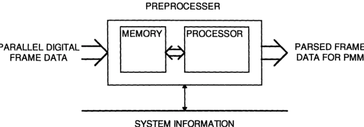
The Preprocessing Module

I

Figure 2.5 Block Diagram of the Preprocessing Module

The preprocessing module is used as a pixel distribution system. It removes the digital frame data stored by the Frame Storage Module and performs any filtering, converting, and parsing necessary to make the data suitable for the Pattern Matching

Module, see Figure 2.5.

The processing system does not have to be very complex; it must have a substantial amount of memory and be fast enough to keep up with the Frame Storage Module. The amount of memory must be sufficient to hold all of the pixel data for two complete frames and all of the associated buffers. All of the pixel data extracted by the Preprocessor is in single bytes, thus any filtering and converting will not involve floating point computations (or floating point processor.) The last function of the Preprocessor is parsing. The digital frame data will be broken up into smaller blocks that the Pattern Matching Module (PMM) will process. The Preprocessor must be able to easily send data to the PMM and keep track of its status in order to make the most efficient use of the Preprocessor to PMM pipeline.

In our application there are many suitable microprocessors and hardware that could easily serve as the Preprocessor. The most important feature is it's memory access and data transfer speeds.

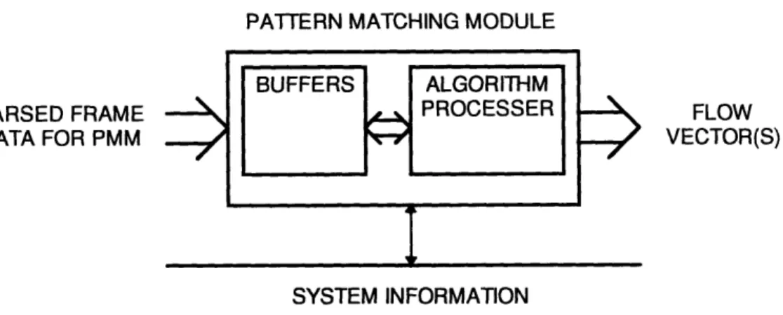
The Pattern Matching Module

PATTERN MATCHING MODULE

PARSED FRAME

DATA FOR PMM

SFLOW

I

SYSTEM INFORMATION

Figure 2.6 Block Diagram of the Pattern Matching Module

The Pattern Matching Module (PMM) finds a data block from one frame in a search window from another frame, see Figure 2.6. The algorithm used to find the new location of the data block is given in Equation 1.15. If the size of the data block is kept relatively small the algorithm does not need any floating point processing support.

The PMM needs to be able to calculate the algorithm fast enough to keep up with the ability of the Preprocessor and Frame Storage Module. The shear number of calculations necessary in the algorithm and the frequency that the algorithm must be used tell us that a dedicated piece of hardware must be used as the PMM, and it must be very fast.

The PMM would be loaded with a search window and a data block; it could compute the best match location without any extra support. This is a key point, viewing the PMM as a black box allows us to use many PMM's in various configurations. Obviously, an important ability of the PMM is to combine more than one PMM in parallel.

All of these issues apply to our application. We want a fast stand alone PMM with the ability to be easily integrated into a parallel system.

43

BUFFERS ALGORITHM

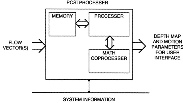
The Postprocessing Module

Figure 2.7 Block Diagram of the Postprocessing Module

The Postprocessing Module will collect all of the data from the PMM(s) and compute the six motion parameters, see Figure 2.7.

The motion parameter calculation, Equation 1.24, involve a large number of calculations; it will need floating point ability as well as the ability to handle large matrix manipulations. The Postprocessor, like the Preprocessor, must be constantly aware of the PMM(s) state in order to make good use of the PMM to Postprocessing gate. Equally important, the Postprocessor must have an efficient way to receive data from the PMM(s). The PMM calculations and the Postprocessing form the largest computational bottlenecks for the Vision System.

In our application the Postprocessor is very similar to the Preprocessor, except that it must be able to process large mathematical computations quickly, and does not require as much data memory.

44

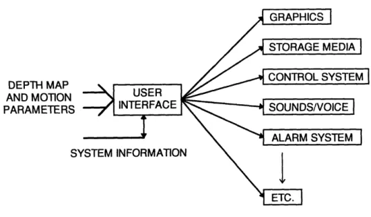
The User Interface

DEPTH MAP AND MOTION PARAMETERS

SY

Figure 2.8 The Infinite Interface

The User Interface would receive the digital information generated about the motion parameters and the obstacle depth map and present them to the system requiring the results. In essence, this is the overall strength on this vision system, the interface can have many different forms depending on the functional need.

The most common use for the system will be as a navigational aid to an autonomous system. The autonomous system could be a sophisticated robotic platform or possibly a blind person; in either case a visual interface is not necessary. The robotic platform would merely like the digital data reflecting the motion parameters as well as the depth map. A blind person, however, may require a tone in each ear indicating the relative proximity to the nearest obstacles, and perhaps a supplementary voice for any additional information.

A visual interface is much more challenging because of the way that this information can be conveyed to a person viewing it. One useful way would be to generate a three dimensional obstacle map in which a simulation of the system using the vision system could be placed.

45

I

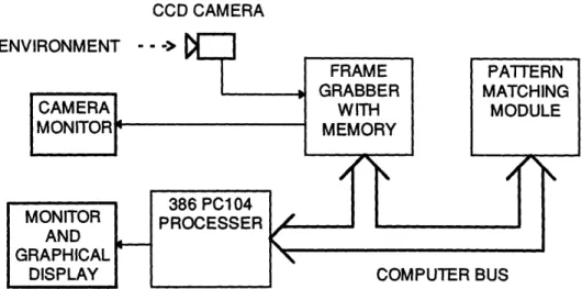
The Prototype Vision System Architecture

CCD CAMERA

E

Figure 2.9 The Prototype Vision System Architecture

After considering all of the possibilities involved in constructing a Vision System a proof of concept system was constructed, see Figure 2.9.

It is a monocular vision system that has a single black and white CCD camera, frame grabber, pattern matching module, and processor. The frame grabber and PMM are at different address locations on the processor's bus; this simple architecture was used to develop the basic hardware and software necessary for a completely functional vision system.

The Vision System functions in the following way. The camera is operating constantly, converting the environment into a video signal. The Frame Grabber, on command from the processor, grabs two frames and stores them in memory. The processor then removes, filters, and parses each frame into its own memory. The parsed frames are fed through the PMM in datablock - search window pairs and the results are stored into the processors memory. After all of the flow vectors have been stored the processor runs the motion algorithm in Figure 1.6 to calculation the motion parameters and the depth map. Once the depth map and motion parameters have been calculated they can be used in any imaginable way.

In terms of the functional components listed in Figure 2.1, the PC104 processor serves as the Preprocessing, Postprocessing, and User Interface Modules. It is a very simple system that can be made quickly and robustly.

The ultimate strength in using this architecture for the prototype system is that all of the pieces of the system can be simulated in software before they are constructed in hardware; this is made easy because we have a centralized single processor system The simulation flexibility also allows the developer to test alternate hardware architectures and troubleshoot both the hardware and software more easily.

Chapter Summary

The chapter began by discussing the natural image processing flow of a general Vision System. The functional components of the natural flow are the Environment Imager, Image Storage Module, Preprocessor, Pattern Matching Module, Postprocessor, and User Interface.

The Environment Imager is used to convert an optical image of the environment into an analog signal. A typical environment imager is a black and white CCD camera. The most important considerations in using a CCD camera for imaging are the shape of the cells in the CCD array, the resolution of the CCD, the ability to control the amount of light the enters the camera, and the ability to improve the image contrast.

The Image Storage Module is used to digitize the analog signal from the Environment Imager and store the information. The design issues involved with Image Storage Module are the type of storage medium, frame or conversion rate, and the generated pixel resolution.

The Preprocessing Module retrieves, filters, and parses the pixel data created by the Image Storage Module. The Preprocessor needs to have a significant amount of memory and speed. It does not have to support floating point calculations.

The Pattern Matching Module is used to generate flow vectors that will make up our motion field. It performs this function by finding a given pattern, called a datablock, in a specific range, called a search window. The location of the datablock in the search window is the flow vector. The primary concerns about the PMM are that it can process quickly and act as a stand alone unit. The black box approach to the PMM will allow it to be used in a parallel architecture.

The Postprocessing Module will calculate the motion parameters. The Postprocessor needs to support floating point and matrix computations.

The User Interface is the most elegant part of the whole system. It can be tailored for any application where there is a need for navigational information. One example as that the User Interface could supply information to the navigational control system of an

autonomous vehicle.

The end of the chapter is a brief introduction to the prototype Vision System constructed for this thesis. The prototype architecture is the simplest way to implement

this proof of concept Vision System. It is a monocular Vision System with a single camera, Frame Grabber, Pattern Matching Module, and Processor. The single processor performs the Preprocessing, Postprocessing, and User Interface functions. The camera, of

course, serves as the Environment Imager. The Frame Grabber, with internal memory, performs the function of the Image Storage Module, and the Pattern Matching Module is itself. The prototype architecture is easy to develop because every component can be simulated in software before being built. The ability to accurately model each component in software also helps troubleshoot the hardware being developed as well as test different hardware architectures.

CHAPTER THREE

THE PROTOTYPE VISION SYSTEM HARDWARE

This chapter contains all of the specific details in the design and construction of the prototype Vision System hardware described in chapters one and two. The system is discussed in two parts, hardware and software; this chapter is dedicated to the hardware development. Both the hardware and the software chapters adhere to the same progression that was used in chapter two, where design decisions of each component are presented sequentially. Figure 2.9 is included again as Figure 3.1 for reference. The intent of this chapter is to provide enough information so that the reader will have a complete understanding of the prototype system hardware.

It should be stressed that any single block in Figure 3.1 has to be designed, or specified, in conjunction with all of the blocks that it interfaces with. The system design issues will be individually addressed for each component.

CCD CAMERA

Figure 3.1 The Prototype Vision System Architecture

3.1 The Prototype Hardware

Figure 3.2 Conceptual Hardware Block Diagram

PC104 PATTERN MATCHING MODULE -PC104 FRAME GRABBER AND COMPUTER 3.5 INCH FLOPPY AND SCSI HARDRIVE

3.2

CCD Camera

The CCD camera is used as the Environment Imager. The camera that was chosen is a PULNiX TM7-CN. (See Figure 3.4) The TM7-CN can be used as a normal video camera, but is tailored for machine vision systems.

Figure 3.4 Pulnix Black and White CCD Camera Component Specifications and Features

e768 horizontal pixels by 494 vertical pixels *Camera is for Black and White applications

*Rectangular CCD cells 8.4.tm horizontal by 9.8*tm vertical *Camera provides Auto Iris feature for lens

'Camera has Gamma contrast control *CCD is 0.5 inches square overall *Very small package

*CCD is sensitive to 1 LUX Design Reasoning

The reasoning for the selection of the camera is based around what we need from our environment. Cameras are instantly divided into two camps -black and white,

sometimes called monochrome, and color. In reality, our machine vision system is only observing the gross movements of the camera through its' surroundings; this motion can be measured with a basic black & white camera. The computational overhead to process color is exactly three times as much -this alone makes it prohibitive since we are aiming for a fast stand alone vision processing system. The next issue is that of image resolution.

The number of horizontal and vertical pixels of the PULNiX TM7 is ample enough for the proposed camera and Frame Grabber system; the Frame Grabber, which has not been discussed in detail yet, has a lower resolution on its best setting and thus will not be "creating" pixels from wholly interpolated data. This is a strange point. The issue is that the camera creates an analog signal from its discreet number of CCD cells. The analog signal produced by the camera from discreet data is intentionally, and even unintentionally by loading, smeared to make it appear smooth. The Frame Grabber can produce any number of pixels from the smeared video signal since it is analog. It makes sense, however, that the Frame Grabber should not try to extract more pixels from the video signal than were used to create it. In our system the resolution of the video camera is sufficient and a more expensive camera would not yield better performance.

As was mentioned in Chapter Two, it is convenient to choose a black and white camera with a simple pixel geometry, auto iris, and contrast control. The easiest pixel geometry to work with is square pixels which for most applications is the best choice. The TM7 does not have exactly square pixels even though it does contain a 0.5 inch square CCD. The TM-7 has 768 horizontal pixels by 494 vertical pixels. The auto iris feature controls the amount of light that hits the CCD. The camera's electronics measure the overall pixel intensity and open and close the lens iris to make full use of the CCD's dynamic range, down to 1 LUX. The last technical point is the ability to increase the camera contrast; the TM7 does this through a Gamma control that increases or decreases the contrast. Finally, the TM7 comes in a very small package that could be used for almost any autonomous application.

3.3 Auto Iris Lens

The lens that was chosen is a Computar MCA0813APC.(See Figure 3.5) Computar lenses are fairly popular for black and white camera applications. Often, they are used on the surveillance cameras at Automatic Teller Machines (ATM).

Figure 3.5 Computar Auto Iris Lens

Component Specifications and Features *Auto Iris for pixel light metering control e8.5 millimeter focal (i.e. wide angle view lens) eAdjustable video signal level

*Auto Close on power down Design Reasoning

The reasoning here is very direct. The most important features are the Auto Iris and focal length.

The Auto Iris feature gives the camera the ability to react to changing light conditions the way the human eye does. Our pattern matching method depends upon matching pixel brightness patterns. Since we expect to eventually use the system on a robotic platform in environments with varying light conditions, we need to be able to maintain, or slowly vary, the relative brightness of the pixels on our CCD. If our robotic