Evaluation of methods to detect interhemispheric asymmetry on cerebral perfusion SPECT: application to epilepsy.

HAL Id: inserm-00136496

https://www.hal.inserm.fr/inserm-00136496

HAL is a multi-disciplinary open access archive for the deposit and dissemination of sci-entific research documents, whether they are pub-lished or not. The documents may come from teaching and research institutions in France or abroad, or from public or private research centers.

L’archive ouverte pluridisciplinaire HAL, est destinée au dépôt et à la diffusion de documents scientifiques de niveau recherche, publiés ou non, émanant des établissements d’enseignement et de recherche français ou étrangers, des laboratoires publics ou privés.

Evaluation of methods to detect interhemispheric

asymmetry on cerebral perfusion SPECT: application to

epilepsy.

Bérengère Aubert-Broche, Pierre Jannin, Arnaud Biraben, Anne-Marie

Bernard, Claire Haegelen, Florence Prigent Le Jeune, Bernard Gibaud

To cite this version:

Bérengère Aubert-Broche, Pierre Jannin, Arnaud Biraben, Anne-Marie Bernard, Claire Haegelen, et al.. Evaluation of methods to detect interhemispheric asymmetry on cerebral perfusion SPECT: application to epilepsy.. Journal of Nuclear Medicine, Society of Nuclear Medicine, 2005, 46 (4), pp.707-13. �inserm-00136496�

I

in SPECT

Evaluation of Interhemispheric Asymmetry

Detection Methods in Cerebral Perfusion

SPECT - Application in Epilepsy

Bérengère Aubert Broche, PhD

; Pierre Jannin, PhD

; Arnaud Biraben, MD

; Anne-Marie

Bernard, MD

_{; Claire Haegelen, MD}

_{; Florence Prigent Le Jeune, MD}

_{; Bernard Gibaud,}

PhD

1

Laboratoire IDM, UPRES 3192, Inserm ESPRI, Faculté de Médecine, Université de Rennes 1, Rennes, France 2

Service de Neurologie, CHU Pontchaillou, Rennes, France 3

Service de Médecine Nucléaire, Centre Eugène Marquis, Rennes, France 4

Service de Neurochirurgie, CHU Pontchaillou, Rennes, France

Bernard Gibaud responsible for correspondence (bernard.gibaud@univ-rennes1.fr)

Laboratoire IDM, Faculté de Médecine, 2, avenue du Pr. Léon Bernard, CS 34317, 35043 Rennes Cedex, France Telephone Number: +33 2 23 23 47 18

Fax number: +33 2 23 23 45 86

6054 words

HAL author manuscript inserm-00136496, version 1

HAL author manuscript

Journal of nuclear medicine : official publication, Society of Nuclear Medicine 04/2005; 46(4): 707-13

HAL author manuscript inserm-00136496, version 1

HAL author manuscript

ABSTRACT

Detecting perfusion interhemispheric asymmetry in neurological nuclear medicine imaging is an interesting approach in epilepsy. Methods: In this study, four methods which detect interhemispheric asymmetries of brain perfusion in SPECT are compared. The first method (M1) is the conventional side-by-side expert based visual interpretation of SPECT. The second method (M2) is the visual interpretation assisted by an interhemispheric difference volume (IHD volume). The last two are automatic methods: the third (M3) is an unsupervised analysis using volumes of interest and the fourth (M4) is an unsupervised analysis of the IHD volume. The comparison of these methods was performed on simulated SPECT data sets by controlling presence and location of asymmetries. The four methods were used to detect a possible asymmetry on 60 simulated SPECT data sets either with or without perfusion asymmetry. From the detection results, Localization ROC (LROC) curves were generated and areas under curves (AUC) were estimated and compared. Finally, these four methods were applied to analyze interictal SPECT data sets in order to localize the epileptogenic focus in temporal lobe epilepsies. Results: This study showed an improvement in asymmetry detection in SPECT images with the methods using IHD volume (M2 and M4) in comparison with the other methods (M1 and M3). However, the most useful method for analyzing clinical SPECT data sets appears to be visual inspection assisted by the interhemispheric difference volume (M2) since the automatic method using the IHD volume (M4) is less specific. Conclusion: The use of quantitative methods can improve perfusion asymmetry detection performance in relation to visual inspection.

INTRODUCTION

The investigation of intractable partial epilepsy is based on a combination of video-EEG (e.g. clinical observation correlated with EEG) and imaging findings. The efficiency of 99mTechnetium HMPAO (Hexa Methyl Propylene Amine Oxime) and 99mTechnetium ECD (Ethyl Cysteinate Dimer) SPECT imaging has largely been demonstrated for detecting perfusion abnormalities and helping to identify the epileptogenic focus (1).

In clinical routine, the analysis of brain SPECT images is often limited to qualitative

side visual inspection. This analysis is user-dependent and involves subjectivity in the interpretation. In this context, quantification might thus improve diagnostic accuracy.

Because the relationship between blood flow and 99mTc-HMPAO or 99mTc-ECD SPECT brain uptake is non-linear due to a saturation phenomenon, absolute measurement of regional cerebral blood flow (rCBF) from HMPAO/ECD SPECT scans is not feasible. Therefore, relative quantification methods are often proposed. Region of interest (ROI) or volume of interest (VOI) based methods (2-4) are used for either intra-scan studies or inter-scan studies (intra or inter subjects). The term “intra-scan” characterizes an analysis limited to a single scan. The term “inter-“intra-scan” refers to an analysis involving several scans. Similarly, “Intra-subject” denotes analysis limited to a single subject, whereas “inter-subject” denotes analysis involving datasets obtained in several subjects. Voxel-based methods are used to study inter-scan only. In the detection of epileptogenic foci, an intra-subject voxel-based method consists in subtracting ictal and interictal SPECT, after they have been coregistered to MRI

(5-6). Inter-subject approaches consist in a comparison between scans of epileptic subject(s) and a control

group (7).

The aim of this paper is to compare the performances of four methods highlighting intra-scan interhemispheric variations in SPECT imaging: the conventional side-by-side visual interpretation by an observer (M1), visual interpretation assisted by the interhemispheric difference volume (IHD volume created by the unsupervised voxel neighborhood method described in (8)) (M2), an unsupervised analysis using volumes of interest (M3) and an unsupervised analysis of the IHD volume (8) (M4).

These methods were compared using simulated SPECT data sets including known asymmetries, and on clinical SPECT data sets with cerebral blood flow variations difficult to see with the naked eye (interictal SPECT scans of patients with temporal lobe epilepsy).

MATERIALS AND METHODS

Perfusion Interhemispheric Asymmetry Detection Methods

side-by-side comparison. This analysis was done by four observers experienced in image analysis: two nuclear medicine physicians, a houseman in neurosurgery and a neurologist.

SPECT data set and the interhemispheric difference volume (IHD volume) were inspected simultaneously by the observer.

The goal of the IHD volume (8) was to help detect perfusion interhemispheric asymmetries in brain SPECT images, using anatomical information available from magnetic resonance images (MRI). For this purpose, the IHD volume was computed at the MRI spatial resolution. For each MRI voxel, the anatomically homologous voxel in the contralateral hemisphere was identified. Both homologous voxel coordinates were then mapped into the SPECT volume using SPECT-MRI registration. Neighborhoods were then defined around each SPECT voxel and compared. A relative difference value was thus computed from both neighborhoods and assigned to the MRI voxel to obtain the volume of interhemispheric differences (IHD volume).

Approaches based on the optimization of statistical similarity measurements have produced accurate SPECT-MRI registration (9). Using realistic simulations of normal and ictal SPECT, we compared the spatial accuracy of major similarity-based registration methods used for SPECT/MRI registration, namely mutual information (10), normalized mutual information (11), correlation ratio (12) and Woods’ criterion (13). Apart for Woods’ criterion, we found similar accuracy for these methods (14). We thus chose to perform rigid SPECT-MRI registration using maximization of mutual information as described by (10).

For every voxel of the MRI volume, the voxel which was anatomically homologous in the contralateral hemisphere is identified, using the spatial normalization scheme provided in the

Statistical Parametric Mapping (SPM) software package (15). This method consists in computing a non-rigid transformation between the MRI scan of the patient and the T1 template (average of 152 normal MRI scans after realignment with the Talairach system) which had been modified in order to be symmetrical. Using this transformation, the voxel corresponding to each point of the patient’s MRI was identified in the template. Since the template was modified to be symmetrical in construction, the homologous voxel in the contra-lateral hemisphere was obtained by symmetry over the sagittal plane. Using the inverse transformation (calculated from the T1 template to the MRI scan), the coordinates of the homologous voxel in the patient’s MRI were determined. The voxel coordinates were then transferred to the already coregistered SPECT volume to define voxel-neighborhoods.

Two symmetrical spherical voxel-neighborhoods (diameter of 18mm) containing 33 voxels were defined on SPECT data around the two homologous voxels. The empirical means (x₁ and x₂) of the voxel SPECT intensity values in both neighborhoods were calculated and the normalized

difference D defined by 1 2 1 2

x x x x

D= ₊− was deduced. This result was stored in a volume of differences at the same coordinates as the initial voxel within the MRI volume (Fig. 1). The calculation was repeated for each MRI voxel in a brain mask to fill the IHD volume.

M3: Automatic VOI-based method Sixty-three anatomical structures, or VOIs (Volumes of Interest)

of intra- and extra-cerebral anatomical structures were hand-drawn and labeled by Zubal et al. (16) from a high-resolution 3D T1-weighted MRI of a healthy subject (124 axial slices, matrix: 256*256,

voxel size: 1.1*1.1*1.4 mm3). This labeled anthropomorphic model of the head is called the Zubal phantom.

To perform SPECT measurements in the VOIs (Fig. 2), the spatial normalization method described by Friston et al. (15) and implemented in the Statistical Parametric Mapping software (SPM99) was used. Both SPECT data and VOIs were spatially normalized to a mean anatomical reference volume, represented by the T1 template provided by SPM, as follows. A non-linear geometric tranformation was estimated to match the 3D T1-weighted MRI of the Zubal phantom, and thus the VOIs, on the SPM T1 template. A two-step approach was used to achieve spatial

normalization of SPECT data. First, an inter-modality/intra-patient rigid registration was performed between each patient’s SPECT and MRI data, by maximization of mutual information. Second, each subject’s 3D T1-weighted MRI was spatially normalized to the SPM T1 template, using a non-linear geometric transformation.

These linear and non-linear geometric transformations were used to resample the SPECT data and the Zubal’s predefined VOIs in the SPM T1 template using trilinear interpolation.

For a spatially normalized Zubal’s predefined VOI and spatially normalized SPECT data, we estimated the mean of the voxel SPECT intensity values (x) within the considered VOI. For each pair

of lateralized VOIs, the empirical means (x₁ and x₂) were calculated and the normalized difference D

was deduced ( 1 2

1 2 100

x x x x

D= −₊ ∗ ).

M4: Automatic IHD volume-based method The unsupervised analysis of the interhemispheric difference volume (IHD volume, detailed in section 2) consisted in studying the voxel of the IHD volume with maximum intensity. VOIs are used to give the anatomical localization of this voxel. As the VOIs are in the T1 template anatomical reference, IHD volume was also spatially normalized to this T1 template.

Evaluation Method

Simulated data-sets To determine and compare the ability of the four methods to detect perfusion

asymmetry zones of various sizes and amplitudes, 40 SPECT data sets including known perfusion asymmetries (in size and amplitude) were simulated. In the same way, 20 SPECT data sets without perfusion asymmetry were simulated.

Realistic analytical SPECT simulations require an activity map representing the 3D spatial distribution of the radiotracer and the corresponding attenuation map describing the attenuation properties of the body.

The attenuation map was obtained by assigning a tissue type to each VOI of Zubal’s phantom (conjunctive tissue, water, brain, bone, muscle, fat, and blood). Each tissue type was assigned an attenuation coefficent µ at the 140 keV energy emission of 99mTc : connective tissue (µ = 0.1781

cm−1), water (µ = 0.1508 cm−1), brain (µ = 0.1551 cm−1), bone (µ = 0.3222 cm−1), muscle (µ = 0.1553 cm−1), fat (µ = 0.1394 cm−1) and blood (µ = 0.1585 cm−1).

To construct the theoretical activity map, a theoretical model of brain perfusion, mimicking mean normal perfusion, was established from real SPECT data (27 healthy subjects) as presented in (17). This involved these SPECT data being spatially transformed into a mean anatomical reference volume and quantitative measurements being taken using the anatomical entity masks extracted from the labeled MRI, after spatial normalization.

From the theoretical activity map, we introduced a single perfusion asymmetry zone of various sizes and intensities in the gray matter of the frontal, occipital, parietal or temporal lobes. The asymmetric zones were spheres with a radius of 5, 10, 15 or 20 mm, defined on the activity map. To model realistic perfusion abnormalities, only gray matter voxel values were increased or decreased (baseline activity plus or minus 10 %, 20 %, 30 % or 40 %). With 4 possible sizes (from spheres with a radius of 5, 10, 15 or 20 mm), 8 possible intensities (baseline activity plus or minus 10 %, 20 %, 30 % or 40 %) and 4 possible localizations (frontal, occipital, parietal or temporal lobes), 128 data sets including a single perfusion asymmetry could be simulated. The 40 data sets used in this study were randomly simulated from these 128 possible data sets.

These attenuation and activity maps were used to simulate SPECT projections taking into account non uniform attenuation (64 projections 128 x 128 over 360°, RecLBL software package (18)). Collimator and detector responses were simulated using an 8mm full width at half maximum (FWHM) Gaussian filter. Poisson noise was also included on these projections. Images were reconstructed using filtered back-projection with a Nyquist frequency cutoff ramp filter and the reconstructed images were postfiltered using a 3D Gaussian filter with full width at half maximum of 8.8 mm, leading to a resolution of 12 mm. Through construction, the simulated SPECT were perfectly aligned with the Zubal phantom MRI.

Data analysis For visual inspection (methods M1 and M2), four clinicians analyzed 60 simulated

SPECT data sets either with or without perfusion asymmetry in the temporal, frontal, parietal or occipital lobe. They were blinded to the patients clinical data. The reading was taken in two

independent steps: with and without the assistance of the IHD volume. The clinicians answered whether the image actually showed asymmetry using a certainty scale from 1 to 5, defined as 1: definitely no, 2: probably no, 3: possibly yes, 4: probably yes and 5: definitely yes. In addition, for scores from 3 to 5, readers indicated the asymmetry location (temporal, frontal, parietal or occipital lobe).

The unsupervised analysis of the interhemispheric difference volume (M4) consisted in studying the voxel of the IHD volume with maximum intensity D. This voxel could be located in a lobe (temporal, frontal, parietal or occipital) or elsewhere in the brain. For the VOI-based method (M3), the normalized difference D was computed for lateralized frontal, occipital, parietal and temporal lobe VOIs. Only the VOI with the highest D value was studied. For these two automatic methods, 4 cutoff values were applied to D to obtain values distributed along the 5 certainty levels, as it is the case for the clinicians answers for methods 1 and 2.

For each score used as a threshold and for each volume, the detected abnormality could be compared to the known asymmetry. Sensitivity (defined as the percentage of simulated data sets for which asymmetries were properly detected and localized) and specificity (defined as the percentage of simulated data sets without asymmetry for which no asymmetry was detected) were determined.

Method comparison The comparisons between the different methods were assessed using

Localized Response Operating Characteristic (LROC) curves (19). LROC curves were deduced by plotting the true positive rate (or sensitivity) against the false positive rate (1 - specificity) for the different thresholds. The area under LROC curves (AUC) was used as an index characterizing the detection performance of the methods. The LROC curves and AUC values obtained for the four methods were deduced and compared.

Clinical Application

Patients and data acquisition Interictal scans of 18 patients (8 women, 10 men, range 14-44 years,

mean: 25 years) with temporal lobe epilepsy (TLE, Right TLE: 8 patients, Left TLE: 10 patients) were included in this study. Four patients had a lesional area and four underwent

ElectroEncephaloGraphy (SEEG). The duration of epilepsy was from 2 years to 37 years (mean: 15.6 years). All patients underwent successful resection (seizure-free after at least two years from the surgery), so the area of resection was then assumed to include the localization of the epileptogenic focus.

For these eighteen TLE patients, interictal SPECT images were acquired with a two-head DST-XL imager (General Electric Medical Systems) equipped with Fan Beam ultrahigh-resolution collimators (13 patients) or ultrahigh-resolution parallel collimators (5 patients). The radiotracer (740

MBq) was 99mTc-HMPAO (3 patients) or 99mTc-ECD (15 patients). Sixty-four projections over 360° (128 128× matrix for 15 patients, 64*64 matrix for 3 patients; pixel size: 4.51 mm for 13 patients, 3.39 mm for 2 patients and 6.78 mm for 3 patients) were acquired. T1-weighted 3D MRI was also performed with a 1.5T Signa machine (General Electric Medical Systems): 124 sagittal 256 256×

slices, voxel =

0 9375 0 9375 1 3mm

.

× .

× .

α

SPECT data were reconstructed using filtered backprojection with a ramp filter (Nyquist frequency cutoff). The reconstructed data were post-filtered with an 8mm full width at half maximum (FWHM) 3D Gaussian filter. The acquisition of linear sources using the clinical acquisition and reconstruction protocols yielded a spatial resolution of FWHM = 12.2mm in the reconstructed images. Assuming uniform attenuation in the head, first-order Chang attenuation correction (20) was performed.

Data analysis Firstly, the four analysis methods were used to detect potential perfusion asymmetry

in the temporal lobes of patients (laterality study). Secondly, these methods were used to localize potential hypoperfusion more precisely in the different regions of the temporal lobe (inner, outer and/or polar, Fig. 3) that had undergone a corticectomy (localization study).

For methods M1 and M2, two observers (observer 1 and 2 of the previous study) analyzed the color SPECT data and IHD volume (for method M2) merged with the MRI data. For the laterality study, they indicated whether or not hypoperfusion was present in the temporal lobe and, where applicable, the hemisphere concerned. For the localization study, they specified whether or not

hypoperfusion was present for each region of the temporal lobe (inner, outer, and/or polar). The degree of concordance between the two observers can be measured using a Cohen's kappa coefficient, using two categories defined as : "observer in agreement with surgery" versus "observer not in agreement with surgery". It shows that the use of the IHD volume led to an increase of kappa from 0.34 (visual inspection) to 0.769 (visual inspection + IHD volume).

For method M3, based on the study of volumes of interest, the interhemispheric difference D was calculated for the volume of interest including the entire temporal lobe for the laterality study and for the inner, outer and polar regions for the localization study (Fig. 5). If the difference D was greater than 5%, the right region was considered to have hypoperfusion, if the value was less than -5%, the left region was considered to have hypoperfusion, if the value was between -5 and 5%, hypoperfusion was considered non-detected. For method M4, based on the study of IHD volume, the analysis focused on the highest intensity voxel (i.e. the highest interhemispheric difference D) in the volume of interest of the entire temporal lobe for the laterality study and in the inner, outer and polar temporal regions for the localization study. If the value of this voxel was less than -20% in the right region, this region was considered to have hypoperfusion. If the value was less than -20% in the left region, this region was considered to have hypoperfusion. If the value was greater than -20%, hypoperfusion was considered non-detected. For methods M3 and M4, the threshold values (5 and 20%, respectively) were chosen experimentally to give the highest possible sum of sensitivity and specificity.

RESULTS

Evaluation of Simulated SPECT Data

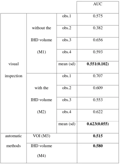
For three of the four observers (observers 1, 2, and 4), the values of the areas under the LROC curves (Table 1) were higher with visual inspection assisted by IHD volume (M2) than with visual inspection alone (M1). According to the value of the area under the curve obtained (from the highest to the lowest), the methods from the most to the least effective were visual inspection assisted by IHD volume (average AUC: 0.62), automatic inspection of the IHD volume (0.58), visual inspection alone

(0.55 on average) and lastly automatic inspection based on volumes of interest (0.51).

Clinical Application

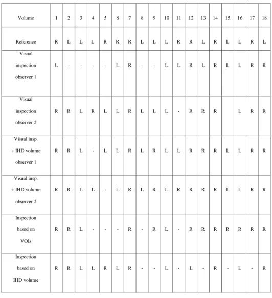
Laterality study We compared the results obtained (presence and laterality of hypoperfusion) with the laterality of the epileptogenic focus, validated by patient recovery following surgery. Table 2 shows these results for the four methods and the two observers.

This enables us to define three cases:

• i: hypoperfusion was identified in the same hemisphere as surgery (ipsilateral

detection),

• c: hypoperfusion was identified in the contralateral hemisphere in relation to surgery,

• n: no hypoperfusion was identified.

This enabled us to calculate the ipsilateral detection fraction (idf), the contralateral detection fraction (cdf) and the no detection fraction (ndf) for each of the analysis methods, as defined in the

following: idf = Number of i cases_{Total cases} , cdf = Number of c cases_{Total cases} and ndf = Number of n cases_{Total cases} . The value of these fractions were computed for the four methods and the two observers (Fig. 4).

Localization study For each patient and temporal region that underwent a corticectomy, we sought

to find out whether hypoperfusion was detected by the different methods. The regions concerned by a corticectomy could be either the outer part of the temporal lobe, the inner and the outer parts, or the inner, outer, and polar parts. Thus, for all the data, a total of 41 regions were studied. Fig. 5 shows the value of the ipsilateral detection fraction (idf), the contralateral detection fraction (cdf) and the no detection fraction (ndf) computed for the 41 regions that underwent a corticectomy leading to patient recovery.

DISCUSSION

Use of the IHD volume, whether automatic (method M4) or in addition to visual inspection of SPECT data (method M2) would appear relevant. Indeed, the values of the areas under curves obtained for simulated data are higher with methods M2 and M4 than with the visual method alone (M1) or the automatic method using volumes of interest (M3). The automatic method (M4) studying IHD volume only retains the most intense asymmetry, regardless of its size, since this study solely focused on the voxel with the highest negative difference. Given that interhemispheric difference is computed over a neighborhood (of 18 mm in diameter), this voxel with the highest intensity is never an isolated point, but rather the center of a high intensity region.

The lower specificity of the automatic method (M4) in relation to the visual method (M2) produces a lower area under curves value for method M4 than for method M2 (0.58 for method M4 and 0.62 on average for method M2). One possible explanation is the fact that the observers confined their study to the four brain lobes whereas the automatic method analyzes asymmetry for the entire brain, thereby increasing asymmetry detection potential. In fact, for 10 of the 60 volumes simulated, the most intense asymmetry detected by the automatic M4 method is located outside the four brain lobes. Moreover, unlike the automatic method, the observers are in a better position to ascertain whether or not the asymmetries observed are actually realistic.

The method M2 has some variable parameters. The size of the spherical voxel neighborhood used to compute difference volumes (diameter 1.8 cm, 33 voxels) was a trade-off: indeed it was large enough to take into account the spatial resolution of SPECT (12.2 mm) and to provide a sufficient number of measures, but not too large in order not to smooth and hide local differences. The plane of symmetry was defined on the MRI template but could also be defined on the SPECT template. We believe that the passage on the MR data yields greater accuracy, although we did not study it. As a matter of fact, if the difference is not significant in term of detection performances, the method could be applied also in situations where no MRI data are available.

Given the large number of simulations to be performed, we opted for an analytical simulation method. Besides modeling acquisition geometry, these simulations model attenuation, Poisson noise

on projections and loss of spatial resolution. The Monte Carlo simulations are more realistic since they are used to model stochastic aspects related to photon emission, propagation and interactions. Nevertheless, we believe that this improvement in the realism of the simulation process does not affect the relative performances of the different methods studied.

The simulated perfusion asymmetries are of various sizes (from 1 to 11cm3) and amplitudes (baseline activity plus or minus 10 %, 20 %, 30 % or 40 %). In a previous study (17), interhemispheric asymmetries on Zubal’s VOIs in ten ictal SPECT of TLE patients were measured, and led to the same order of magnitude. However, it is difficult to demonstrate the realism of these asymmetries. The only thing we can say about it, is that according to the clinicians, the sizes and contrasts of asymmetries met in epilepsy look similar to those simulated. Of course, it would have been possible to simulate multiple asymmetry zones but we were not interested in this case, since most epileptic patients show one epileptic focus only, and complex cases with multiple foci are not candidate to a surgical treatment.

For 10 simulated data sets, the changes to the activity map are of very low amplitude (plus or

minus 10% of activity). For 9 other data sets, the changes are very slight (approximately 1cm3). It is therefore only natural that these are not detected, which explains the low values of the areas under curves obtained for all the methods.

For the simulated data, the method based on the use of volumes of interest (M3) proved less effective than the other methods. We believe that this result is due to the fact that the regions were too large for the asymmetries sought. This is the key problem with analyses based on the study of volumes of interest: finding a suitable volume size (21-22). Thus, on the clinical data, between the hypoperfusion lateralization and localization studies, the temporal lobe regions were resegmented. In the hypoperfusion localization study, the no detection fraction was significantly lower than in the lateralization study (12% and 33%, respectively, for the same detection threshold). We believe that the regions are too large for analyzing lateralization, and that therefore the method’s sensitivity is inadequate (sensitivity of 44% with the large temporal lobe region in the lateralization study and 56% with the resegmented regions in the localization study), for the same threshold. The results therefore show that it is necessary to redefine the regions to achieve a better analysis. However, it is often

difficult to adapt the regions to the size of the asymmetries sought, which is rarely known.

If we study the results of the four observers for the simulated data in detail, differences can be seen from one observer to another. For three observers (observers 1, 2, and 4), performance improves in terms of area under curves between the analysis of data alone (M1) and data analysis assisted by IHD volume (M2). Observer 3 achieved inferior performances for analysis assisted by IHD volume (M2) but the best performances for data analysis alone. The difference between the results can depend on the observers’ epileptological experience and the difficulty involved (according to the observers) in choosing one asymmetry, as at times they thought they could find several. Thus, the criterion for choosing asymmetry may be thought to vary from one observer to the next (e.g. the most intense, the most extensive, a compromise between the two). Inter-observer variability is slightly less important for analysis with IHD volume than without using it: 3 or 4 observers gave identical findings (in terms of localization or absence of localization) for 37 of the 60 data sets without the use of IHD volumes and for 41 of the 60 data sets using IHD volumes. As for the simulated data, the analysis of clinical data with IHD volume tends to produce uniform observer results. Indeed, for the laterality study, with visual analysis alone (M1), the observers give an identical result for 8 volumes and with the visual analysis assisted by IHD volume (M2), identical results were achieved for 15 volumes. For the localization study, these results were 23 and 30 volumes, respectively.

The tracer and SPECT parameters were unfortunately not consistent for the 18 patients. One cannot exclude that this might affect the analysis. For example, the difference of fixation between the two tracers (HMPAO and ECD) could modify the interhemispheric perfusion asymmetry values. Moreoever, it could be possible that the volume or the pixel size have an impact on detection performances, via the registration accuracy. We have not enough data to do a complete statistical analysis, but it would be interesting to study the impact of the different parameters as well as the relation between the results obtained and some clinical parameters (as duration of epilepsy or the presence of a lesion).

The use of interhemispheric asymmetry detection methods is particularly relevant for interictal SPECT analysis, since such data show slight cerebral blood flow variations, that may easily be missed by the clinician in absence of a suitable quantification tool. In practice, the reduction of sensitivity due

to the specific case of bi-lateral abnormalities should not really be a problem, at least in the context of epilepsy, since other exploration techniques are available (such as depth electrodes recordings) to detect this situation. So, we feel that the study of these interictal clinical data for patients suffering from temporal epilepsy is of particular interest in studying concordance between observers and methods. However, although epilepsy laterality and the precise localization of the epileptogenic focus are validated by patient recovery following surgery, we cannot know whether hypoperfusion really exists at this focus in the interictal period. Interictal hyperperfusion is also described in the literature in a small proportion of patients only. It can affect the epileptogenic zone or occasionally a different region, even the contralateral region (1). As it is unusual to record clinical EEG simultaneously, we cannot know whether or not there is a subclinical discharge at the time of injection. In Devous’ meta-analysis (1), an interictal hypoperfusion is found in 43% of cases compared on surgical outcome. In our data series, some methods produce higher sensitivity. Indeed, good laterality detection values range from 39% with the volumes of interest-based method, to 67% with the visual analysis of observer 2 assisted by IHD volume.

So, in summary, intra-scan investigation for detecting perfusion interhemispheric asymmetries proves very useful for pathologies such as focal epilepsy, particularly in cases of slight cerebral blood flow variations, as is the case with temporal epilepsy in the interictal period (in temporal epilepsy, the asymmetry is very obvious in the ictal period) or frontal epilepsy in ictal and interictal periods. The principle of the methods presented is to detect all asymmetries, which can be pathological or normal (23). To determine whether or not an asymmetry is pathological, the detected asymmetries need to be compared with those obtained from a population of healthy subjects (24), which brings another family of inter-scan, inter-subject methods into play.

CONCLUSION

We have shown that the use of quantitative methods can improve perfusion asymmetry detection performance in relation to visual inspection and, in particular, can help to delimit these regions better with a view to surgery. The comparison of the proposed methods shows that the most

appropriate method for clinical analysis of SPECT data is the visual method with additional "assistance" for analyzing data, namely in this study, a volume giving interhemispheric differences (IHD volume). This method is also useful for increasing concordance of results produced by observers.

REFERENCES

1. Devous MD, Thisted RA, Morgan GF, Leroy RF, Rowe CC. SPECT brain imaging in epilepsy: a meta-analysis. J Nucl Med. 1998;39:285–293.

2. Baird AE, Donnan GA, Austin MC, Hennessy OF, Royle J, McKay WJ. Asymmetries of cerebral perfusion in a stroke-age population. J Clin Neurosci. 1999;6:113–120.

3. Kuji I, Sumiya H, Niida Y et al. Age-related changes in the cerebral distribution of 99mTc-ECD from infancy to adulthood. J Nucl Med. 1999;40:1818–1823.

4. Migneco O, Darcourt J, Benoliel J et al. Computerized localization of brain structures in single photon emission computed tomography using a proportional anatomical stereotaxic atlas. Comput Med Imaging Graph. 1994;18:413–422.

5. Zubal IG, Spencer SS, Imam K, Seibyl J, Smith EO, Wisniewski G and Hoffer PB. Difference images calculated from ictal and interictal technetium-99m-HMPAO SPECT scans of epilepsy. J Nucl Med. 1995;36:684–689.

6. O’Brien TJ, So EL, Mullan BP et al. Subtraction ictal SPECT co-registered to MRI improves clinical usefulness of spect in localizing the surgical seizure focus. Neurology. 1998;50:445–454.

7. Lee JD, Kim HJ, Lee BI, Kim OJ, Jeon TJ, Kim MJ. Evaluation of ictal brain SPET using statistical parametric mapping in temporal lobe epilepsy. Eur J Nucl Med. 2000;27:1658–1665.

8. Aubert-Broche B, Grova C, Jannin P et al. Detection of inter-hemispheric asymmetries of brain perfusion in SPECT. Phys Med Biol. 2003;48:1505–1517.

9. Barnden L, Kwiatek R, Lau Y et al. Validation of fully automatic brain SPET to MR co-registration. Eur J

Nucl Med. 2000;27:147–154.

10. Maes F, Collignon A, Vandermeulen D, Marchal G, Suetens P. Multimodality image registration by maximisation of mutual information. IEEE Trans Med Imaging. 1997;16:187–198.

11. Studholme C, Hill DLG, Hawkes DJ. An overlap invariant entropy measure of 3D medical image alignment.

Pattern Recognition. 1999;32:71–86.

12. Roche A, Malandain G, Pennec X, Ayache N. The correlation ratio as a new similarity measure for

multimodal image registration. MICCAI 1998 Cambridge, Lecture Notes in Computer Science, Springer, 1998;1496:1115–1124.

13. Woods RP, Mazziotta JC, Cherry SR. MRI-PET registration with automated algorithm. J Comput Assist

Tomogr. 1993;17:536–546.

14. Grova C, Jannin P, Buvat I, Benali H, Gibaud B. Evaluation of registration of ictal SPECT/MRI data using statistical similarity methods. MICCAI 2004 Saint Malo, Lecture Notes in Computer Science, Springer, 2004;3216:687-695.

15. Friston KJ, Ashburner J, Poline JB, Frith CD, Heather JD, Frackowiak RSJ. Spatial registration and normalization of images. Hum Brain Mapp. 1995;2:165–189.

16. Zubal IG, Harrell CR, Smith EO, Rattner Z, Gindi GR and Hoffer PB. Computerized three-dimensional segmented human anatomy. Med Phys. 1994;21:299–302.

17. Grova C, Jannin P, Biraben A et al. A methodology for generating normal and pathological brain perfusion SPECT images for evaluation of MRI/SPECT fusion methods: application in epilepsy. Phys Med Biol.

2003;48:4023–4043.

18. Huesman RH, Gullberg GT, Greenberg WL, Budinger TF. RECLBL library users manual, Donner

algorithms for reconstruction tomography. Technical-report pub 214, Lawrence Berkeley Laboratory, University of California, 1977.

19. Starr SJ, Metz CE, Lusted LB, Goodenough DJ. Visual detection and localization of radiographic images.

Radiology. 1975;116:533–538.

20. Chang LT. A method for attenuation correction in radionucleide computed tomography. IEEE Trans Nucl Sc. 1978;25:638–643.

21. Kang KW, Lee DS, Cho JH et al. Quantification of f-18 FDG PET images in temporal lobe epilepsy patients using probabilistic brain atlas. Neuroimage. 2001;14:1–6.

22. Stamatakis EA, Wilson JT, Hadley DM, Wyper DJ. Spect imaging in head injury interpreted with statistical parametric mapping. J Nucl Med. 2002;43:476–483.

23. Van Laere K, Versijpt J, Audenauert K et al. 99mTc-ECD brain perfusion SPET: Variability, asymmetry and effect of age and gender in healthy adults. Eur J Nucl Med. 2001;28:873–887.

24. Van Bogaert P, Massager N, Tugendhaft P et al. Statistical parametric mapping of regional glucose metabolism in mesial temporal lobe epilepsy. Neuroimage. 2000;12:129–138.

Figure 1. Creation of the inter-hemispheric difference volume (IHD volume): (1) identification of homologous voxels (2) transfer of the MR voxel coordinates to the SPECT volume (SPECT-MRI registration) (3) definition of the voxel neighborhoods (4) calculation of the normalized difference, stored in the difference volume at the same coordinates as the initial voxel within the MR volume.

Figure 2. VOI-based method

Figure 3. Representation of an axial slice of temporal volumes of interest from MRI data (A): the volume of interest including the entire temporal lobe (in purple) is represented in (B). The right image (C) represents the inner (light green), outer (blue), polar (bright green) and posterior (purple) temporal regions.

Figure 4. Laterality of potential hypoperfusion in the temporal lobe: comparison of the four detection methods based on clinical data in terms of ipsilateral detection fraction (idf), contralateral detection fraction (cdf) and no detection fraction (ndf). For the first two methods involving a human observer, performances are given for the two observers.

Figure 5. Localization of potential hypoperfusion in the different parts of the temporal lobe: comparison of the performance of four detection methods based on clinical data in terms of ipsilateral detection fraction (idf), contralateral detection fraction(cdf) and no detection fraction (ndf). For the first two methods involving a human observer, performances are given for two observers.

AUC

obs.1 0.575

without the obs.2 0.382

IHD volume obs.3 0.656

(M1) obs.4 0.593

visual mean (sd) 0.551(0.102)

inspection obs.1 0.707

with the obs.2 0.609

IHD volume obs.3 0.553

(M2) obs.4 0.622

mean (sd) 0.623(0.055)

automatic VOI (M3) 0.515

methods IHD volume

(M4)

0.580

Table 1. AUC

Volume 1 2 3 4 5 6 7 8 9 10 11 12 13 14 15 16 17 18 Reference R L L L R R R L L L R R L R L L R L Visual inspection observer 1 L - - - - L R - - L L R L R L L R R Visual inspection observer 2 R R L R L L R L L L - R R R L R R Visual insp. + IHD volume observer 1 R R L - L L R L R L L R R R L L R R Visual insp. + IHD volume observer 2 R R L L - L R L R L R R R R L L R R Inspection based on VOIs R R L - - - R - R L - R R R R R R R Inspection based on IHD volume R R L L R L R - - L - L - R - L - R

Table 2. Laterality of potential hypoperfusion in the left (L) or right (R) temporal lobe obtained using the different methods for eighteen interictal data sets ("-": no hypoperfusion detected). The reference given is

the lobe that contained the epileptogenic focus and underwent a corticectomy leading to patient recovery.