HAL Id: hal-01364026
https://hal.archives-ouvertes.fr/hal-01364026
Submitted on 3 Nov 2016
HAL is a multi-disciplinary open access
archive for the deposit and dissemination of
sci-entific research documents, whether they are
pub-lished or not. The documents may come from
teaching and research institutions in France or
abroad, or from public or private research centers.
L’archive ouverte pluridisciplinaire HAL, est
destinée au dépôt et à la diffusion de documents
scientifiques de niveau recherche, publiés ou non,
émanant des établissements d’enseignement et de
recherche français ou étrangers, des laboratoires
publics ou privés.
Event-Based Sampling Algorithm for Setpoint Tracking
Using a State-Feedback Controller
Fairouz Zobiri, Nacim Meslem, Brigitte Bidégaray-Fesquet
To cite this version:
Fairouz Zobiri, Nacim Meslem, Brigitte Bidégaray-Fesquet.
Event-Based Sampling Algorithm
for Setpoint Tracking Using a State-Feedback Controller.
EBCCSP 2016 - 2nd IEEE
Confer-ence on Event-Based Control Communication and Signal Processing, Jun 2016, Cracovie, Poland.
�10.1109/EBCCSP.2016.7605235�. �hal-01364026�
Event-Based Sampling Algorithm for Setpoint
Tracking Using a State-Feedback Controller
Fairouz Zobiri
Univ. Grenoble Alpes Laboratoire Jean Kuntzmann
and GIPSA-lab
CS 40700, F-38058 Grenoble Cedex 9 Email: [email protected]
Nacim Meslem
Univ. Grenoble Alpes GIPSA-lab
F-38000 Grenoble, France. Email: [email protected]
Brigitte Bidegaray-Fesquet
Univ. Grenoble Alpes Laboratoire Jean Kuntzmann CS 40700, F-38058 Grenoble Cedex 9
Email: [email protected]
Abstract—Event-based control techniques are investigated
for output reference tracking in the case of linear time-invariant systems. In event-based control, the controller remains at rest if the system is behaving according to some predefined conditions, the feedback loop being closed only when the system states violate these conditions. In this work a reference system, which consists in the continuously-controlled version of the system under study, is employed. Based on the difference between the state of the event-triggered system and that of the reference system, we define a Lyapunov-like function, and show that if we can keep this function confined to a certain region, the tracking error would also be bounded. The trespassing of this function outside of the desired region is used as an event-triggering condition.
I. INTRODUCTION
Event-based control is a control strategy in which the control law is updated following the occurence of an event related to the state of the system under study. It has appeared in the last decades as an appealing alternative to periodic control. The ever-growing number of publications on the topic ( [1], [2], [3], [4], [5] and references therein) testifies of this shift of interest away from periodic control. By periodic control, we refer to the classical approach that consists in uniformly sampling a control law in order to transfer it onto a digital platform. The discretization is thus carried out by taking a sample value of the continuous-time signal at fixed time intervals. Of course, the popularity of this approach is due, apart from its orderly nature, to the fact that it has been exhaustively investigated for several decades.
However, lately, the control community has been pon-dering over the shortcomings of the periodic implementa-tion in modern control facilities. First, periodic sampling requires the use of a very small time-step in order to satisfy the Nyquist–Shannon sampling theorem and keep the properties of the original, continuous-time signal. But, this is often met with hardware limitations, as the sampling period can only get as small as the hardware resolution allows it to. Then, in a modern industrial environment, applications are often set to communicate through a band-limited (sometimes wireless) network, where transferring data at a very high rate may lead to the congestion of the network [6], possibly resulting in disastrous consequences on the behavior of the interconnected systems. It also represents a considerable waste of energy, along with all
its environmental and economical implications.
From such conclusions stemmed the idea that control should only be applied when needed. In event-triggered control, the value of the control signal is kept constant as long as the system does not undergo any significant change. A new sample of the control signal is taken when the state of the system reaches unacceptable values or when some stability condition is violated. During the time the control is held unchanged, the controller is at rest, and no state measurement is fed back to it, reducing thus energy consumption and reducing the load on the communication channels. It has also the merit of being a more intuitive approach, as humans tend to turn their attention on tasks that need intervention rather than on those which are run-ning smoothly. However, it does present the disadvantage of having to monitor the state of the system continually.
Up to now, the research on event-based strategies has been focused on stability and stabilization issues ( [7], [8], [9], to name a few). Inspired by results developed in the literature, we introduce an event-based approach for output tracking of a reference trajectory by a linear time-invariant (LTI) system.
A few works on event-based control for reference track-ing do exist throughout the literature. For instance, in [10], an event-based LQR controller is implemented, while the reference tracking is achieved through integral action. In [11], [12], [13], an additional fictitious system that generates the desired trajectory is defined. The event-triggering con-ditions are then established according to the error between the state of the reference system and that of the actual system.
In all these approaches, the reference system is chosen to be an external system, that would suit the purpose of analysis. In this work though, we propose to select the reference system as the continuously-controlled version of the event-triggered system being considered. It is indeed reasonable to assume that the behavior of the continuously-controlled system should serve as a role model for the per-formance of the event-based algorithm. Our main objective then would be to maintain the tracking error between the states of the two systems under a certain bound. This is done by noticing that this error can be viewed as the state of a new virtual system, and will ultimately decay to zero if the system is stable. The practical stability of the error-related system is then guaranteed by associating a Lyapunov-like
function to it, which would be kept from increasing above a certain level, defining thus our triggering conditions.
This work is organized as follows: in the next section we expose the mathematical framework of the problem at hand by explaining the event-based scheme. In section III, we define the event-triggering conditions that ensure the boundedness of the error. Some simulation results are then presented in section VI.
II. PROBLEMSTATEMENT
Let us consider the LTI system described as follows ˙
x(t ) = Ax(t) + Bu(t),
y(t ) = C x(t), (1) x(t ) ∈ Rn is the state vector, y(t ) ∈ Rp is the system output and u(t ) ∈ Rm is the control input.
We wish to drive the output of system (1) to asymp-totically follow a trajectory determined by an exogenous signal r (t ), denoted as the reference input. We first define the reference system which consists in system (1) for which the control law is classically defined as
ur(t ) = −K x(t) +Gr (t), (2)
where K ∈ Rm×n is the feedback gain and G ∈ Rm×p is a calibration matrix, where G = (−C (A − BK )−1B )−1.
As a result, we obtain the following closed-loop system ˙
xr(t ) = (A − BK )xr(t ) + BGr (t),
yr(t ) = C xr(t ),
(3) such that
1) (A − BK ) is Hurwitz with desired eigenvalues, 2) limt →∞kyr(t ) − r (t)k = 0.
The control law ur(t ) is applied continuously to system (1) and classical control theory affirms that achieving 1) and 2) is always possible when the pair (A, B ) is controllable. We assume in what follows that it is the case for system (1).
In event-based control, however, the control is updated only at some time instants tk, k ∈ N, when certain condi-tions on the behavior of the plant are no longer satisfied, resulting in time instants tkwhich are not necessarily evenly spaced. The control input, now denoted by ¯u(t ), is defined
at time tk by ¯
u(tk) = −K x(tk) +Gr (tk). (4) It is maintained constant on time intervals [tk, tk+1):
¯
u(t ) = ¯u(tk) ∀t ∈ [tk, tk+1). (5) Then system (1) becomes
½x(t ) = Ax(t) + B ¯˙ u(t k),
y(t ) = C x(t), t ∈ [tk, tk+1), k ∈ N.
(6)
As mentioned previously, we consider the continuously-controlled system (3) as a reference system, meaning that, at each time instant, the behavior of the event-based system will be compared to that of the reference system. From this comparison, we will determine whether the behavior of system (6) is acceptable or whether the control should be updated.
Remark 1. The principle of a reference system in the
event-based scheme has also been used in references [11], [12], [13]. Our approach differs in the fact that the reference system is provided within the method, whereas in [11] and [12] the choice of the reference system is left for the user to make. The work presented in [13] deals with a stability problem since the states are driven to zero.
Since we have assumed that all the conditions are united to achieve limt →∞kyr(t ) − r (t)k = 0, it is sufficient to guarantee that limt →∞ky(t ) − yr(t )k = 0, to ensure that the output y(t ) of the event-triggered system follows the trajectory of r (t ).
In this work, however, we consider the more general problem of driving the state error kx(t) − xr(t )k to zero as time t tends to ∞. This principle is depicted in Fig. 1. From the relationship between x(t ) and y(t ) shown in system (1), we deduce that limt →∞kx(t )− xr(t )k = 0 implies limt →∞ky(t ) − yr(t )k = 0.
Notice that for the plants where the states are not available for measurement, techniques for obtaining an estimation of these states (such as observers) do exist and can be used alongside our approach with only a small modification.
Defining the event-triggering conditions is the topic of the next section.
III. EVENT-TRIGGERINGCONDITIONS FORTRACKING A
REFERENCEINPUT
In this section, we define a new system based on the reference and the event-based systems. The state of this new system, the error between the real state x(t ) and the reference state xr(t ),
e(t ) = x(t) − xr(t ), (7) will serve as a basis for updating the control ¯u(t ). The
behavior of the error signal e can be described as follows 1) when t ∈ (tk, tk+1)
˙
e(t ) = (A − BK )e(t) − BK ∆kx(t ) + BG∆kr (t ), (8a)
where∆kx(t ) = x(tk) − x(t), ∆kr (t ) = r (tk) − r (t), 2) when t = tk, k = 0,1,2,...
˙
e(t ) = (A − BK )e(t). (8b)
Remark 2. Throughout this work, we allow the exogenous
signal r (t ) to be only piecewise Lipschitz, and we authorize it to contain jumps, provided that there exists a minimum interval of time between two successive jumps where r (t ) is continuous. Moreover, we require the signals used as exogenous inputs r (t ) to be uniformly bounded.
Remark 3. Note also that despite the jumps in r (t ), the
states xr(t ), x(t ) and e(t ) remain Lipschitz. However, their first derivatives do exhibit jumps. Indeed, jumps in ˙x(t )
occur when an event happens and jumps in ˙xr(t ) are due to jumps in r (t ). Therefore ˙e(t ) exhibits jumps both when
r (t ) Mux ˙ xr= (A − BK )xr+ BGr yr= C xr ˙¯ u(t ) = 0 ¯ u(tk) = −K x +Gr ˙ x = Ax + B ¯u y = C x y xr Event Generator V (e(t )) = δ x x(t )
Fig. 1. Schematic of the proposed event-based tracking controller.
Based on equation (8b), we can associate to the system (8) a Lyapunov-like function of the following form
V (e(t )) = e(t)T P e(t ), (9) where P , a symmetric positive-definite matrix, is a solution to the Lyapunov equation
(A − BK )TP + P(A − BK ) = −Q, (10)
where Q is a positive-definite matrix.
Equations (9) and (10) stem from the fact that V (e) should be a positive-definite function, whose first time-derivative is non-positive. These conditions, according to Lyapunov’s theory, are sufficient to guarantee the stability of system (8).
In our approach though, we do not try to prevent
V (e) from increasing, but we show that we are capable of
maintaining V (e) confined within a certain region. In other words, between two time instants tk and tk+1, V (e) may increase; but, whenever V (e) reaches a certain upper bound, the control is updated, forcing V (e) back inside the chosen region. This concept is illustrated in Fig. 2.
Letδ > 0 be the upper limit that we want to achieve on
V (e),
0 ≤ V (e) ≤ δ. (11)
From equation (9) we can deduce that the Lyapunov-like function V (e) is naturally bounded as follows
λmin
P ke(t )k
2
≤ V (e) ≤ λmaxP ke(t )k
2, (12)
where λminP and λmaxP are, respectively, the smallest and largest eigenvalues of matrix P . Since P is positive-definite, its eigenvalues are real and positive.
By requiring that V (e) be bounded from above, and from inequality (12), we can guarantee an upper bound on the error e(t ), expressed as
ke(t )k ≤ s δ λmin P = ². (13)
Consequently we can define our triggering conditions based on this premise.
Definition 1. We define the time-instant tk+1 (k ∈ N) at which the control-law ¯u(t ) is updated as the minimum time
time 0 1 2 3 4 5 0 0.1 0.2 0.3 0.4 0.5 0.6 V(e) Upper Limit
Fig. 2. Example of the evolution of the Lyapunov equation under our triggering conditions.
instant t > tk for which V (e(t )) = δ:
tk+1= inf{t > tk,V (e(t )) = δ}. (14) Theorem 1. If the event-based control ¯u(t ) is updated
according to the event-triggering condition defined in (14), then the tracking error e(t ) remains confined in the ball of radius ², i.e.
ke(t )k ≤ ², (15)
for² defined by (13).
Proof: To prove Theorem 1, we study the time derivative
of the Lyapunov-like function V defined by equation (9). Since the matrix P is positive-definite, for all e ∈ Rn, V (e) ≥ 0. At time t0, e(t ) is chosen to be zero (we assume x(t0) =
xr(t0)). Then, at time t = tk, when V (e(t )) reaches the value
δ the control is updated such that
˙
V (e(t ))|t =tk = ¡ ˙e(t)TPe(t ) + e(t)TP ˙e(t )¢
|t =tk
= e(tk)T(A − BK )TPe(tk) +e(tk)TP (A − BK )e(tk) = −e(tk)TQe(tk).
From equation (10), the matrix Q is symmetric positive-definite, meaning that ˙V (e) is negative-definite, V (e(t ))
comprised between the lines V (e(t )) = 0 and V (e(t)) = δ. Since Q is a positive-definite matrix, its largest and small-est eigenvalues, λmaxQ and λminQ , respectively, are real and positive. Then, we can set an upper and lower limit on the descent of V (e(t )),
−λmaxQ ke(tk)k2≤ −e(tk)TQe(tk) ≤ −λminQ ke(tk)k2. (16) We have demonstrated earlier that in this region ke(t)k ≤ ². Thus ˙V (e(t ))|t =tk≤ −λmin
Q ²2 for all k.
However, the boundedness of the tracking error e(t ) is not sufficient to deem the triggering condition in Defini-tion 1 appropriate. We need also to guarantee that under these triggering conditions, there exists a minimum time lapse between two update instants. This extra requirement avoids, to borrow the terminology of hybrid systems, Zeno phenomena, where an infinite number of updates is needed within a finite interval of time. This also allows to give an estimation of the number of necessary updates of the control, for the purpose of minimizing the communication cost of the event-triggered control.
We can prove the existence of this minimum delay in the case when r (t ) is Lipschitz.
Theorem 2. Let r (t ) be a Lipschitz input signal. Then, there
exists a minimum timeτmin> 0, independent of k, such that
∀k ∈ N, tk+1− tk> τmin,
where the tk, k ∈ N are defined in Definition 1.
Remark 4. Assuming that r is Lipschitz is not a very strong
assumption, since in practice, a low-pass filter is used on the reference input to handle the abrupt changes that it may contain and avoid actuator saturation, eventually rendering it Lipschitz.
Proof: We show that there exists τ independent of k
such that ˙V (e(t )) remains negative in the interval t ∈ [tk, tk+
τ). We will necessarily end up having τ < τmin. For t > tk, ˙
V (e(t )) = −e(t )TQe(t )
−2∆kx(t )TKTBTPe(t ) + 2∆kr (t )TGTBTPe(t ) ≡ −e(t )TQe(t ) + Rk(t ).
We prove that there exist β > 0 and τ1> 0, independent of
k, such that for all t ∈ (tk, tk+ τ1), −e(t)TQe(t ) < −β, and
0 < τ2< τ1 such that for all t ∈ (tk, tk+ τ2), |Rk(t )| < β/2. Hence for t ∈ (tk, tk+ τ2), ˙V (e(t )) is uniformly bounded
from above by −β/2.
To determine τ1, we have to prove that ke(t)k2 remains
relatively large on some time interval. From equations (11), (12), and (16)
−e(tk)TQe(tk) ≤ − λmin Q δ λmax P . We therefore consider β = λQminδ/2λmaxP .
To have −e(t)TQe(t ) < −β it suffices to show that ke(t)k >
qβ/λmin
Q =qδ/2λmaxP . We can rewrite ˙e(t ) as
˙
e(t ) = (A − BK )e(t) + Fk(t ), (17)
where
Fk(t ) = −BK ∆kx(t ) + BG∆kr (t ).
In order to find a bound on Fk(t ), we need the following lemma.
Lemma 1. If r (t ) is an Lr-Lipschitz function, then the following assumptions are verified.
(i) There exists Lr> 0 such that
k∆kr (t )k ≤ Lr(t − tk). (18) (ii) As noticed in Remark 3, x is Lipschitz. Let Lx be its
Lipschitz constant. Therefore,
k∆kx(t )k ≤ Lx(t − tk). (19) From Lemma 1, we can state that
kFk(t )k ≤ BK Lx(t − tk) + BGLr(t − tk) ≤ C τ1,
· being the subordinated matrix-norm in Rn×nandRn×p, and C constant. For t ∈ (tk, tk+ τ1), we can also write an
integral formula for (17), namely
e(t ) = e(A−BK )(t−tk)e(t
k) + Z t tk e(A−BK )(t−s)Fk(s)d s. Since A − BK is Hurwitz, ke(t )k ≥ ke(tk)k −C τ12.
From (12) we also know that ke(tk)k ≥qδ/λmaxP . Therefore for a sufficiently small τ1, which does not depend on k, we
can ensure that
ke(t )k ≥ q
δ/2λmax
P and hence −e(t)TQe(t ) < −β.
We then move on to prove that |Rk(t )| is bounded from the above by β/2. |Rk(t )| ≤ 2PBK ke(t)kk∆kx(t )k +2P BGke(t )kk∆kr (t )k ≤ 2 s δ λmin P τ2(k|P BK k|Lx+ P BGLr) , and it is easy to chooseτ2small enough such that |Rk(t )| <
β/2 for t ∈ (tk, tk+ τ2).
Remark 5. The proof of Theorem 2 uses in a crucial way
the hypothesis that r is Lipschitz. If r experiences jumps as will be the case in our numerical experiments, it is no more possible to give a lower bound of the delay between two samples. Indeed, although we can estimate | ˙V (e(t ))| by
2PBK ke(t)kk∆kx(t )k + 2PBGke(t)kk∆kr (t )k which can also be bounded by a constant on the time interval [tk, tk+
τ1], we do not master the times at which jumps in r take
place. Typically if it happens very shortly after tk, when
V (e(t )) is very close to δ, the time for V (e(t)) to reach δ
again can be very short and cannot be estimated in terms of the parameters of the system.
IV. SIMULATIONRESULTS
A. Yaw damper example
As an application to our approach, we consider the example introduced in [14]. It is a simplified model of a jet aircraft during cruise flight, with two inputs: rudder and aileron deflections; and two outputs: yaw rate and bank angle. The state-space representation is given in the form of system (1), where A = −0.0558 −0.9968 0.0802 0.0415 0.5980 −1150 −0.0318 0 −3.0500 0.3880 −0.4650 0 0 0.0805 1.0000 0 , B = 0.0729 0.0000 −4.7500 0.00775 0.15300 0.1430 0 0 , C = µ 0 1 0 0 0 0 0 1 ¶ .
We want the outputs to track a certain reference signal
r (t ) ∈ R2, which consists in two step signals that start at
some value and remain constant for half the simulation time, then both jump at half-time to a different value. So, through pole-placement, we design a state feedback control of the form (4) with
K = µ 0.3235 −0.6325 0.1891 0.2561 −12.5446 −0.7213 25.9652 27.2314 ¶ and G = µ −11.7069 0.7115 −202.0659 35.3351 ¶ .
We choose the positive-definite matrix P describing the Lyapunov-like function (9) as P = 4.6408 −0.8446 −0.1942 −0.1980 −0.8446 0.9479 0.2071 0.3299 −0.1942 0.2071 0.6457 0.5917 −0.1980 0.3299 0.5917 4.6188 .
For a maximum tolerance on the error of ² = 0.5, and the selected Lyapunov function, we find δ = 0.1233.
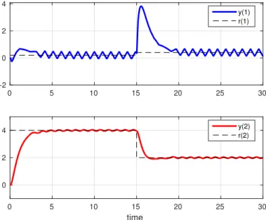
0 5 10 15 20 25 30 -2 0 2 4 y(1) r(1) time 0 5 10 15 20 25 30 0 2 4 y(2) r(2)
Fig. 3. The evolution of the two output signals along with their respective reference signals 0 5 10 15 20 25 30 -2 0 2 4 yr(1) r(1) time 0 5 10 15 20 25 30 0 2 4 yr(2) r(2)
Fig. 4. Outputs of the continuously-controlled system
0 5 10 15 20 25 30 -4 -3 -2 -1 0 1 u(1) time 0 5 10 15 20 25 30 -200 -150 -100 -50 0 50 100 150 u(2)
Fig.3 shows the evolution of the two outputs with respect to time, with each output represented with the reference signal it is supposed to track. We can see that for a relatively large value of δ, the system is able to track the reference, even though the first output y(1) exhibits some ripples. This is due to the large value of δ which results in the fact that the individual updates of the control law are rather spaced in time as shown in Fig.5. However, from Fig. 4, it is obvious that the overall behavior of the system is similar to that of the continuously-controlled reference system. This also shows that the large overshoot experienced by the first output is due to the dynamics of the system and not the event-based scheme.
From Fig.5 we can see that the control updates are unevenly spaced in time. Indeed, during the transient period or when there is an abrupt change in the value of the reference, the control is updated quite often, whereas when the reference settles at a constant value, the updates become less frequent and rather regular in time.
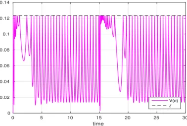
time 0 5 10 15 20 25 30 0 0.02 0.04 0.06 0.08 0.1 0.12 0.14 V(e) δ
Fig. 6. The evolution of the Lyapunov function
Fig.6 shows the evolution of the Lyapunov-like function
V (e(t )) with respect to time. We can notice that it remains
enclosed within the region bounded from above byδ. Fig.7 is a zoom on the graph of V (e) around t = 15, when r jumps to a new value. It can be noticed that V (e) trespasses the boundary set byδ in some instants. This is due to the fact that computer simulations run in discrete-time rather than continuous-time, and therefore, detecting the time at which V (e(t )) reaches the value δ is not possible.
B. Comment on the Discrete Implementation of the System
For obvious practical reasons our simulations are per-formed using an underlying discrete time. For the above simulation this sampling time is ts= 10−4. Besides a nu-merical scheme is used to solve the differential equation, namely a second order Adams–Bashforth scheme (two-step explicit scheme).
For the sake of simplicity let us assume that we use a simple explicit Euler scheme instead. Let tn, n ∈ N be the uniform time sampling at which the computation is
time 14 14.5 15 15.5 16 0.1215 0.122 0.1225 0.123 0.1235 0.124 V(e) δ
Fig. 7. Behavior of the Lyapunov function when a jump in r occurs
performed. Then e(tn) is approximated by en and
en+1− en ts = (A − BK )e n − BK ∆kxn + BG∆kr (tn), tn∈ (tk, tk+1). (20)
Hence, using the Hurwitz property on A − BK , and that in the worst case kenk =qδ/λmaxP
ken+1k ≤ (1 + ts) q δ/λmax P + tsBK Lx(t n − tk) + tsBGBr. This yields an upper bound on the worst value of V (en+1) ≤
λmax
P ken+1k2, which can be bigger than δ. This explains the fact that the Lyapunov function exceeds δ on Fig. 7. We cannot avoid such overflows with explicit numerical schemes. When this happens, tn+1 is chosen as tk+1, and for the computation of en+2 equation (8b) is used. Then
V (en+2) = V (en+1) − tsen+1TQen+1 + ts2V ((A − BK )en+1),
(21) Which can still be aboveδ. A few iterations can be necessary to recover V (en) < δ.
C. Comparing the number of control updates for different values of δ
The number of updates of the control law in a given time interval depends directly on the value ofδ. Selecting a rather largeδ implies that we are allowing a large tolerance on the value of the tracking error e(t ), and consequently, the control law will not need to be updated very often. On the other hand, if we require a smaller tolerance on the error e(t ), the control law will have to be updated more frequently, and this is associated with a small δ. The latter case converges to the continuous-control scheme if we require zero tolerance on the tracking error.
TABLE I illustrates the variations of the number of updates in the control signal for the previous example as we change δ. We run the simulation for a fixed time-span in each case (Tfinal= 30). We have run the simulation at a
time-step of 10−4, thus ending up with 300, 000 simulation
instants.
The table shows that even for very small values of ² and δ, the number of necessary updates in the value of the control remains relatively small compared to the overall
0 5 10 15 20 25 30 -2 0 2 4 y(1) r(1) time 0 5 10 15 20 25 30 0 2 4 y(2) r(2)
Fig. 8. Output signals for² = 0.05 and δ = 0.0012
² δ Number of Updates
0.8 0.316 66
0.5 0.1233 71
0.05 0.0012 304
0.001 4.93 × 10⁻⁷ 19088
TABLE I. NUMBER OF UPDATES OF THE CONTROL SIGNAL FOR DIFFERENT VALUES OF²ANDδ
number of simulation instants.
For example, for² = 0.05, the number of updates is only 304 which is still very small for 300, 000 simulation instants, or a ratio of 1/1000. However, the quality of the tracking is much improved for such value of the tolerance ² and its corresponding δ, as depicted in Fig. 8.
V. CONCLUSION
In this work, we have proposed an event-based imple-mentation for an output tracking problem. We have shown that if we update the control only when the value of a defined Lyapunov-like function reaches an upper limit, we can guarantee a good tracking of the reference signal, with a relatively small number of updates. We can thus reduce the communications between the controller and process as well as the number of operations performed by the controller.
As further work, it would be interesting to consider a variable value of δ. Indeed, if we assume that we have a prior knowledge of the reference input, we can adapt the value of δ accordingly, allowing a larger tolerance when r experiences abrupt changes, and decreasing the tolerance when r is smoother, thus allowing more time for the controller to adapt to the changes in r .
Another idea to explore would be the self-triggered approach. In event-triggered control, even though the con-trol is not updated continuously, the triggering condition is monitored continuously. On the other hand, in a self-triggered scheme, at each update instant we compute not only the control, but also the next instant at which the control would have to be updated, removing thus the obligation to monitor a condition continuously.
ACKNOWLEDGMENT
This work has been partially supported by the LabEx PERSYVAL-Lab (ANR-11-LABX-0025-01).
REFERENCES
[1] K.-E. Årzén, “A simple event-based PID controller,” in IFAC World
Congress, Beijing, China, Jul. 1999.
[2] D. Lehmann and J. Lunze, “Event-based control: A state-feedback approach,” in 2009 European Control Conference (ECC). IEEE, Aug. 2009, pp. 1716–1721.
[3] J. Lunze and D. Lehmann, “A state-feedback approach to event-based control,” Automatica, vol. 46, no. 1, pp. 211–215, Jan. 2010. [4] W. M. Heemels, M. T. Donkers, and A. R. Teel, “Periodic
event-triggered control for linear systems,” IEEE transaction on Automatic
Control, vol. 58, no. 4, pp. 847–861, Apr. 2013.
[5] N. Meslem and C. Prieur, “Event-based controller synthesis by bounding methods,” European Journal of Control, vol. 26, pp. 12– 21, Nov. 2015.
[6] X.-M. Zhang, Q.-L. Han, and X. Yu, “Survey on recent advances in networked control systems,” IEEE Transactions on Industrial
Infor-matics, to appear.
[7] A. Anta and P. Tabuada, “To sample or not to sample: Self-triggered control for nonlinear systems,” vol. 55, no. 9, pp. 2030–2042, Sep. 2010.
[8] A. Girard, “Dynamic triggering mechanisms for event-triggered con-trol,” vol. 60, no. 7, pp. 1992–1997, Jul. 2015.
[9] R. Postoyan, A. Anta, D. Neši´c, and P. Tabuada, “A unifying Lyapunov-based framework for the event triggered control of nonlinear sys-tems,” in 50th IEEE Conference on Decision and Control and European
Control Conference (CDC-ECC). Orlando, FL, USA: IEEE, Dec. 2011,
pp. 2559–2564.
[10] S. Durand, B. Boisseau, J.-J. Martinez-Molina, N. Marchand, and T. Raharijaona, “Event-based LQR with integral action,” in 2014 IEEE
Emerging Technology and Factory Automation (ETFA). Barcelona, Spain: IEEE, Sep. 2014, pp. 1–7.
[11] P. Tallapragada and N. Chopra, “On event triggered trajectory tracking for control affine nonlinear systems,” in 50th IEEE Conference on
Decision and Control and European Control Conference (CDC-ECC).
Orlando, Florida, USA: IEEE, Dec. 2011, pp. 5377–5382.
[12] ——, “On event triggered tracking for nonlinear systems,” IEEE
Transactions on Automatic Control, vol. 58, no. 9, pp. 2343–2348, Sep.
2013.
[13] M. Shao, F. Hao, and X. Chen, “Event-triggered and self-triggered asymptotically tracking control of linear systems,” in 32nd Chinese
Control Conference (CCC). Xi’an, China: IEEE, Jul. 2013, pp. 6650– 6655.
[14] MathWorks. Yaw damper design for a 747® jet aircraft. http://fr.mathworks.com/help/control/examples/yaw-damper-design-for-a-747-jet-aircraft.html.