HAL Id: hal-01407055
https://hal.archives-ouvertes.fr/hal-01407055
Submitted on 1 Dec 2016
HAL is a multi-disciplinary open access archive for the deposit and dissemination of sci-entific research documents, whether they are pub-lished or not. The documents may come from teaching and research institutions in France or abroad, or from public or private research centers.
L’archive ouverte pluridisciplinaire HAL, est destinée au dépôt et à la diffusion de documents scientifiques de niveau recherche, publiés ou non, émanant des établissements d’enseignement et de recherche français ou étrangers, des laboratoires publics ou privés.
A tree-parenchyma coupled model for lung ventilation
simulation
Nicolas Pozin, Spyridon Montesantos, Ira Katz, Marine Pichelin, Irene E.
Vignon-Clementel, Céline Grandmont
To cite this version:
Nicolas Pozin, Spyridon Montesantos, Ira Katz, Marine Pichelin, Irene E. Vignon-Clementel, et al.. A tree-parenchyma coupled model for lung ventilation simulation. International Journal for Numerical Methods in Biomedical Engineering, John Wiley and Sons, 2017, �10.1002/cnm.2873�. �hal-01407055�
1
A tree-parenchyma coupled model for lung ventilation simulation
N. Pozin1,2,3, S. Montesantos3, I. Katz3,4, M. Pichelin3, I. Vignon-Clementel1,2, C. Grandmont1,2
1
INRIA Paris, 2 Rue Simone Iff, 75012 Paris, France
2
Sorbonne Universités, UPMC Univ. Paris 6, Laboratoire Jacques-Louis Lions, 75252 Paris, France
3
Medical R&D, WBL Healthcare, Air Liquide Santé International, 1 Chemin de la Porte des Loges, 78350 Les Loges-en-Josas, France
4
Department of Mechanical Engineering, Lafayette College, Easton, PA, 18042, USA,
Summary
In this article we develop a lung-ventilation model. The parenchyma is described as an elastic homogenized media. It is irrigated by a space-filling dyadic resistive pipe network, which represents the tracheo-bronchial tree. In this model the tree and the parenchyma are strongly coupled. The tree induces an extra viscous term in the system constitutive relation, which leads, in the finite element framework, to a full matrix. We consider an efficient algorithm that takes advantage of the tree dyadic structure to enable a fast matrix-vector product computation. This framework can be used to model both free and mechanically induced respiration, in health and disease. Patient-specific lung geometries acquired from CT scans are considered. Realistic Dirichlet boundary conditions can be deduced from surface registration on CT images. The model is compared to a more classical exit-compartment approach. Results illustrate the coupling between the tree and the parenchyma, at global and regional levels, and how conditions for the purely 0D model can be inferred. Different types of boundary conditions are tested, including a nonlinear Robin model of the surrounding lung structures.
1. Introduction
Lung and respiratory pathologies are a growing concern and considered to be the third cause of death in the world [1]. Although they have been studied for decades some are still not well understood. For instance this seems to be the case for asthma which causes are not consensually understood [2]. Clinical tests are costly and submitted to a strict regulation. Furthermore in-vivo measurements on the lung are tedious. In this context mathematical modeling can provide relevant insights on the lung behavior, especially in pathological situations.
The lung is a complex multi-scale and multi-physics system. It supplies the organism with oxygen by carrying a flow of fresh air through the tracheo-bronchial airway tree. Gas exchange takes place in regions distal to the tree, in the alveoli, which are embedded in a viscoelastic tissue, called the lung parenchyma. Common lung diseases can affect lung ventilation distribution [3], [4] and numerous studies have focused on lung ventilation modeling.
In [5], the lung is modeled as a single viscoelastic compartment fed in gas by a resistive pipe. Although this model is able to recover appropriate tidal tracheal flow and lung volume evolution through the respiration cycle, it does not give insights on regional ventilation. In [6], [7] the single compartment model is extended to a multi-compartment description. The lung is seen as a 0D space-filling resistive branching network feeding independent compliant terminal regions. A possible limitation of this exit compartment model is that it is driven by a pressure forcing term, though no in-vivo experiment provides the spatio-temporal pressure field around the lung. Some studies [8], [9], [10] propose to impose flows issued from image registration as boundary conditions at the tree exits. Ventilation distribution is then computed along the tree. This approach may provide relevant results
2 but it is not predictive. In particular, boundary conditions acquired in a healthy configuration cannot be used to simulate ventilation when airway remodeling occurs. Besides, to distribute the flow obtained from the surface displacement among the different tree exits is not obvious. Another possible limitation of the exit compartment model is that terminal units are mechanically independent from one another; this may not reflect the lobar-level-continuous nature of the parenchyma. Some studies [11], [12] treat the parenchyma as a continuous elastic material but do not consider the effect of the tree on the parenchyma dynamics, though in some pathological cases airway remodeling induces ventilation defaults. In [13] an exit-compartment model in which compartments are mechanically linked through a static equilibrium relation is proposed.
In this work we treat the parenchyma as an elastic media coupled, in the same spirit as [14], to a space-filling dyadic resistive tree. Applying the least-action principle we obtain the equations governing the parenchyma displacement field from which the tracheo-bronchial ventilation is deduced. Equations are solved in a finite element framework and the designed numerical methods take advantage of the dyadic structure of the tree to enable fast computations. To overcome the lack of knowledge on pleural pressure we propose to apply Dirichlet boundary conditions namely the surface displacement of the parenchyma, which can be registered from images at different lung inflation states. We work on physiologically realistic tree and lung geometries segmented from 3D computed tomography (CT) images. We study the influence of airway remodeling on ventilation heterogeneity. Finally, we also investigate the possible limitations of the exit compartment description through a comparison to the tree-parenchyma coupled model.
In Section 2, the theoretical background of the model is presented and the tree-parenchyma coupling governing equations are obtained. An exit compartment model designed for comparison is also described. It assumes alveolar regions are mechanically independent from one another. To enrich the comparison, we show how the tree-parenchyma coupled model can be used in order to compute a pressure forcing term that takes into account the mechanical interaction between alveolar regions and that is applicable to the exit-compartment model. In Section 3, numerical methods used to solve equations of both models are presented. In Section 4, we detail how the space-filling tree and the parenchyma mesh along with its registered surface displacement are built. In Section 5, some numerical examples are presented. We test the tree-parenchyma coupled model in spontaneous tidal breathing conditions with both linear and non-linear flow dissipation models and we study the effect of bronchoconstriction on lung ventilation. Then, we investigate the assumption of mechanical independence between the exit compartments in the eponym model. Based on parenchyma surface image registration, we apply “realistic” Dirichlet boundary conditions and we study the impact of various boundary conditions on the ventilation distribution. Finally we simulate a pressure-controlled mechanical ventilation with boundary conditions that prevent the lung from expanding over total lung capacity.
2. Model
First we present two different ventilation models. Each of them takes into account the compliant behavior of the lung tissue. The first one - called here tree-parenchyma model - describes the parenchyma as an elastic continuous media. The second one, called hereafter the exit compartment model, treats the parenchyma as a set of independent compliant compartments, each of them characterized by a unique compliance coefficient. In both cases the lung tissue receives inhaled air through a branching network of pipes that stands for the bronchial tree. We assume that the air flow in each branch of this dyadic tree is characterized by a resistance, modeling fluid dissipation. In this section, we thus present the resistive tree model, then the tree-parenchyma model and the exit compartment model. The last two models are finally compared and their links explained.
3
2.1. Tracheo-bronchial tree
The air flows through a dyadic branching network (see Figure 1) and we assume its branches to be rigid during the respiration cycle. This assumption is reasonable under tidal breathing conditions as a first approximation and is supported by simulations performed in [7]. Moreover the fluid is assumed to be Newtonian and incompressible. The air incompressibility is justified since the Mach number is much lower than one [15]. We also neglect fluid inertance [7]. Consequently the air flow in each cylindrical branch of the tree can be characterized by a single resistance parameter denoted and the pressure drop along an airway is proportional to the flux within the branch, namely
In the case of Poiseuille flow in a circular branch we have
(1)
where is the fluid dynamic viscosity, and are the pipe’s length and radius, respectively. If only interconnected pipes in which the fluid flow is described by Poiseuille law are considered, one may fail to predict accurately the pressure drops due to bifurcations and to non-linear inertial effects, in particular in the upper airways [16]. In [17] Pedley proposes a non-linear resistance model designed to account for the pressure drop at symmetric bifurcations:
(2)
where and is the Reynolds number defined by with the fluid density. This model is designed to treat bifurcations with a branching angle =70°. However does not significantly impact the pressure drop as noted in [18], so will be used independently of the
angle. Note that the Pedley model was designed for inspiration. Since the aim of the paper is to model the tree-parenchyma coupling and to investigate the possible effects of resistance non-linearities, and not to provide a precise description of pressure drops in the tree, (2) is also used for expiration. Other non-linear resistance laws in the literature [16], [19] could also be readily incorporated in the proposed model.
A human trachea-bronchial tree contains on average 23 generations leading to 223 exits [20]. To reduce the computational cost, starting at a given generation, we condense the subtrees into single equivalent branches, hereafter called tree exits. In distal regions, under tidal breathing, the Reynolds number is low so that Poiseuille law holds true. We also assume that subtrees are symmetrical. As in [20] we assume distal airways resistances follow a geometrical progression with common ratio 1.63. Given those assumptions, a subtree equivalent resistance can be computed according to classical series/parallel resistance network formulas. This requires that outlet pressures within each subtree are uniform; which is usually valid when the subtree is small, i.e when the tree exit generation is high.
Now, following [21], [22], we describe how to link pressure drops between the trachea and the exits, and exit flows. Let be a 0D dyadic tree structure with terminal branches. Let vectors
and , where is the pressure at the trachea entrance, and
4 going from the trachea down to the exit, and the intersection set between and (see
Figure 1).
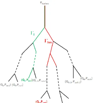
Figure 1: schematic tracheo-bronchial tree representation, from the trachea down to the N exits through each path (example in green). (in red) contains the branches common to the paths and .
Since conducting airways are assumed rigid and gas flow is incompressible, the flow going through a branch equals the sum of the flows going through its daughters. Under these conditions, it can be shown [21]that and are linked by a linear operator that accounts for the tree resistance:
(3)
where with , being the resistance associated with branch k. This
formulation avoids computing the pressure at each tree node as in [7], [14] keeping the number of unknowns tractable. The power dissipated in the tree can be written as
(4)
where is the transposed vector to .
Remark 1: If one wants to take into account airway compliance using, for example, the model
developed in [7], then the mother to daughter flow conservation does not hold anymore; and (3) is no longer valid. However, as shown in Appendix 8.1, by considering the model of [7], the flux loss due to compliant airways is negligible. Nevertheless, to take into account airway compliance, one can consider that the radii in (1) or (2) are given by a quasi-static elastic law; see for instance [23] where such models are described.
Pressure at the trachea is an external force applied to the system. If breathing is spontaneous and without considering the extra-thoracic part, this pressure is a given constant, the atmospheric pressure. The extra-thoracic part could be included as an extra resistance at the trachea level. In case of mechanical ventilation, air is pushed in by the ventilator resulting in an imposed pressure
at the trachea, so Exit tree pressures on the other hand
are unknowns of the system. In the following we show how they can be determined and coupled to the parenchyma.
5
2.2. A tree-parenchyma coupled model
We assume that the lung parenchyma is an isotropic elastic media occupying a 3D domain denoted by . Here, since our aim is to describe the tree-parenchyma coupling, we choose to consider a linearized behavior law and to neglect tissue viscosity. This assumption can be justified when considering normal breathing (see Remark 2). Let us denote the displacement of the parenchyma by defined in , taken as the reference state of the lung. The linearized stress tensor of the media is given by
where and are the effective Lamé parameters of the effective material, and the strain tensor defined by Note that these effective macroscopic coefficients and may be obtained using a homogenization process as described in [24] and [25]. The latter takes into account the alveoli microstructure so that we may refer to the homogenized media when considering the lung tissue. In particular, when the alveoli are assumed to have a hexagonal shape and to be uniform in size then the isotropic behavior of the homogenized law can be derived [24].
As stated above, the lung parenchyma is fed with air that flows through a dyadic resistive tree. If an airway of the tracheo-bronchial tree is nearly closed (due to a stenosis for example) the related fed region will require more effort to stretch, even if its elastic properties are not affected. Hence the parenchyma and the tree models need to be mechanically coupled. Let us assume that
and , for each of the subregions corresponding to one tree exit (see Figure 2). Doing so we neglect the conductive tree volume which is of the order of 100mL [15] and which is indeed much smaller than the overall lung volume (around 5L). We denote the image of through the transformation . Assuming that lung tissue at the microscopic level is incompressible and because of the fluid incompressibility, the volume variation of is equal to the associated fluid flux, namely
where is the volume of . So setting we have
(5) where is the boundary of , is the unit normal vector along and the cofactor matrix of a matrix . Under the hypothesis of small displacements around the reference state, which is assumed to be the initial position, we get
(6) Next, to derive the system of equations describing the time evolution of the coupled tree-parenchyma system, we apply the least-action principle. Since energy is lost in the resistive tree the system is dissipative. In case resistances do not depend on the flow, based on (4), the power lost to friction can be included in the Lagrangian with a Rayleigh dissipation function:
6 where is the vector of elements defined by (6). Next the kinetic and potential energies of our system as well as the work of the external forces can be defined as follows. The kinetic energy of the system is
(8) where is the macroscopic lung parenchyma density. The potential energy of the system is
(9)
where the colon denotes the contraction operation between tensors. Depending on the respiration regime, the chest and diaphragm induce a surface force field, , on the parenchyma, generating or resisting the motion. The associated work is
(10)
that includes the pressure at the trachea introduced previously. The Lagrangian of the tree-parenchyma system S writes
In case dissipative forces are applied to , the Lagrange equation is
(11)
Its weak form reads
(12)
and sufficiently smooth such that and .
From (7) we easily have:
, where is the
piecewise-constant function defined by
From (8) we derive and . From (9) we have
and . From (10) we get and . So (12) reads
7
from which we deduce the weak formulation of the equations satisfied by : being sufficiently smooth (13)
The associated strong formulation then reads:
It is associated with the following Neumann boundary conditions:
Let be the piecewise constant function defined by
(14)
which is the pressure felt by the parenchyma material. Equation (13) then writes:
(15)
The associated strong formulation is:
(16)
It is associated with the following Neumann boundary conditions:
(17)
where is the stress tensor associated with the action of the tree on the parenchyma
(18)
With such a coupling, the displacement field is the only unknown. Note that the approach introduced in [14] and [26] to impose the flux conservation (6) use a Lagrange multiplier, thus introducing new variables. This is not the case here since we have a global formulation describing the fully coupled system. The tree-parenchyma coupling reduces to an apparent piecewise-constant pressure that depends on the flow. The associated volume force is
(19)
The function is defined by (14). Equation (19) is only defined at the distribution level since it is a Dirac on the terminal regions boundaries. The effect of the tree is analog to an apparent pressure exerted on terminal regions boundaries (see Figure 2). Flow dissipation in the tree induces an extra viscous component to the parenchyma constitutive relation: . From the
8 mechanical point of view it makes it harder to expand the effective material during inspiration and to contract it during expiration. Higher flow means more power is required to induce motion. Equation (19) can also be derived from a local energy balance. Moreover, (19) remains valid when depends on the flow, still being given by (14). This generalizes the approach to any airway resistance law, e.g for non-linear models.
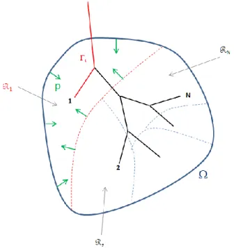
Figure 2: apparent pressure exerted on terminal regions. The domain Ω is occupied by the parenchyma and subdivided into non-intersecting regions Ωi, each of which is fed in gas through the path i. Green arrows represent the apparent pressure p applied on terminal region Ω1 due to the coupling with the tree.
Remark 2: Linear elasticity holds for small displacements around a non-stressed reference position.
The assumption of linear elasticity is supported by the fact that under low tidal breathing frequency motions parenchyma viscosity effects are less marked. Some more realistic viscoelastic non-linear laws could be considered but this work focuses on tree-parenchyma coupling. Moreover there is no consensus on the actual parenchyma constitutive relation, thus the more sophisticated law to be used remains an open question. Besides, the theoretical framework developed hereafter only slightly depends on the constitutive relation. In the case where the constitutive relation is not linear, then is still given by (7) but with given by (5). Finally, , the term of the variationnal formulation relative to the tree, writes .
The derivation has been performed, as an illustration, for a Neumann boundary condition (17). In the case where a pressure field is applied around the parenchyma, is
where corresponds to the pleural pressure field around the parenchyma. However, there is no consensus on the spatio-temporal distribution [27] of this pressure. To our knowledge, non-invasive in-vivo measurements cannot be performed. Other boundary conditions can be applied; in particular we can impose Dirichlet boundary conditions by prescribing the spatio-temporal surface displacement field of the parenchyma:
9
where may be provided by imaging data as we will see in Section Erreur ! Source du renvoi introuvable.. For mechanical ventilation or spirometric tests modeling, Robin boundary conditions can be applied to model the action of the surrounding tissue. Based on [28] we propose non-linear boundary conditions that take into account the chest and the diaphragm resistance to lung expansion. One can consider given by
where is a lobar dependant function that can be for instance be defined by
(20) with the outer surface of lobe i, and respectively the current inhaled volume in
lobe i, its volume at functional residual capacity (FRC) and total lung capacity (TLC). Coefficient is a constant. Its value should be chosen based on physiological considerations, that is to say the compliance of the lung surrounding media: rib cage, diaphragm. At a given volume inflation, function is constant on each lobe: the constraint is assumed to be uniform at a lobar level.
A complete problem statement for this system (16) requires boundary conditions as well as initial conditions. We simulate respiration, which is a periodic phenomenon. This means here that initial conditions will not affect the behavior of the system after a transition period. The initial conditions used herein are simply and .
Instead of considering the parenchyma as a continuum, some models (see [5], [6], [7], [29]) consider a set of mechanically independent compartments. In the following we present an exit-compartment model in the perspective of a comparative study between both descriptions.
2.3. An exit-compartment model
Here, the tracheo-bronchial tree feeds some “balloons” that represent groups of alveolar sacs. They are modeled through a 0D pressure-volume relationship that can incorporate viscous, elastic and inertial effects. This kind of model is based on an inherent assumption: exit compartments are mechanically independent although the lung parenchyma is a continuous media, at least at a lobar level. In this framework, spontaneous ventilation is driven by the pleural pressure evolution, which is, as stated before, challenging to measure. Both the mechanical independence assumption and the lack of knowledge on pleural pressure are possible limitations to the use of such model. In order to investigate these possible drawbacks, an exit-compartment model (see Figure 3) is defined and compared to the previous tree-parenchyma coupling description.
10
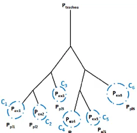
Figure 3: schematic of a 6-exit tree in the frame of the exit-compartment model. The tree feeds gas to independent terminal regions standing for groups of alveolar sacs. Elastic properties of those compartments are accounted for by compliances Ci. Inside each compartment is the alveolar region with pressure Pexi, while outside is the local pleural pressure Ppli.
To make a relevant comparison, the tree description remains unchanged, and as for the parenchyma (see 2.2), terminal balloon dynamics is governed by a linear elastic law. The pressure in the
compartment is linked to the local pleural pressure around the parenchyma through
where and are respectively the current volume and the reference state configuration volume of the compartment. Coefficient is the i’th balloon compliance and quantifies the stiffness of the region. Since compliance is an extensive variable, can be chosen as where is the
lung volume at the reference state and is the total static lung compliance. In a pathological
case where lung tissue properties are locally affected, one can modify regional compliances accordingly.
The pressure drop along the tree according to (3) is
(21)
The pressure drop in the alveolar region is
(22) where ,
and is the diagonal matrix with coefficient on the diagonal element. Denoting , and since , summing up equations (21) and (22) leads to the following system of governing equations:
11 where and .
Remark 3: the balloons compliance could be chosen as current volume dependant in the same
spirit as the Robin boundary conditions described in 2.2. Doing so would take into account that the lung is harder to expand when its volume gets close to the total capacity and harder to contract when its volume gets close to the residual capacity, see [28].
In the following we show how the pleural pressure applied as a forcing term to this exit-compartment model can be computed from the tree-parenchyma coupled model.
2.4. From the tree-parenchyma coupled model to the exit-compartment model
In this section we compute the average pressure endured by terminal region in the tree-parenchyma coupled model. This resulting pressure naturally includes the mechanical connection between alveolar regions and its evolution can be driven by “realistic” Dirichlet boundary conditions (see 2.2). Then is applied as a driving force to the balloon of the exit compartment model. Doing so accounts for mechanical interactions between compartments and avoids the need to know the pleural pressure distribution around the lung.
The pressure applied to the terminal balloon of the exit-compartment model is
where is the parenchyma stress tensor and . As tangential
forces are not included in , energy spent to induce motion might be different in both models although ventilation is the same. We have:
The coupling term is easily computed following (14) and (18),
. In the linear elasticity framework,
where is the elastic pressure associated with the recoil of the material, the
bulk modulus sets a correspondence between Lamé parameters and the local compliance. For a given domain with reference volume we have:
(24)
where, is the Young modulus, is the Poisson ratio. Coefficients and are linked to the Lamé parameters through , .
Under the assumption that elastic pressure is null at equilibrium, it leads to
where is the reference
equilibrium volume of region . To account for a residual pressure at equilibrium a constant can simply be added. We finally end up with a similar equation as (23):
12
(25)
Next, to solve the governing equations presented in the current section, efficient numerical methods are developed.
3. Numerical methods
In this section we describe numerical methods used to solve constitutive equations of both models. The weak form of the equations governing the tree-parenchyma coupled model (see 2.2) is discretized in time and space within the finite element framework. As described below, due to the tree the obtained linear system contains a full matrix. Consequently this can make a direct resolution inefficient. A decomposition of this operator enabling the use of a fast matrix-vector product is thus proposed. The system is then solved iteratively. Iterative methods are not commonly used in elasticity; however, it is possible here since the homogenized material is compressible, and even approaching incompressibility the system can still be solved. The linear system governing the exit-compartment model (23) is discretized in time and efficiently inverted following methods described in [24].
3.1. Tree-parenchyma coupled model
Let be the time step. For any vector we denote its approximation at time . In the following, discretization is performed on the variational form relative to the Neumann pressure boundary conditions case (15). A similar treatment can be applied to other boundary conditions. As in [24] we apply the following time scheme:
(26)
and equation (15) discretized with (26) leads to
When considering non-linear resistances, they are treated explicitly; i.e, to solve the system at step n+1 the resistance matrix (see 2.2) is computed with flows from step n. We get to solve where
and
.
Implementation is performed on our in-house finite element software FELIScE [30]. Lagrangian finite P1 elements are used for space discretization. Decomposition in the finite element basis leads to:
(27)
where is the vector representation of in the FEM .
Matrix stands for the mass and elastic term. It is the FEM matrix associated to the linear form . In the linear elasticity framework we have:
13
(28)
where is the element of the finite element basis.
The matrix represents the coupling term associated to following bilinear form:
where is the m’th component of vector and . So we have:
(29) and finally (30) with
. The decomposition given by (30) is a consequence of the tree
dyadic structure. Note that is a full matrix since the tree couples all the FEM degrees of freedom of the system.
Finally the right hand side of (27) writes:
(31)
Equation (27) is solved through a conjugate gradient method with preconditioning. A Jacobi preconditioner is computed at the first time step and then reused to precondition the system at further time steps. Operator changes at each time step when resistances are non-linear. Assembling and storing would be a highly memory demanding operation. Taking advantage of its decomposition (30) and noticing that is a sparse matrix and is small compared to (the size of is the number of tree exits, which is much lower than the size of the finite element system), we do not assemble and rather compute product through
enabling more efficient computation (see 5.6).
When Dirichlet boundary conditions are applied, the right hand side of (27) is replaced by
14 where and are respectively the displacement and velocity of the parenchyma surface.
Discretizing the variational formulation associated to the Robin boundary condition leads to the following system: (32) with and Where is the trachea pressure for mechanical ventilation. The Robin boundary conditions are
treated implicitly through a fixed-point algorithm with relaxation as illustrated by the following scheme:
Figure 4: resolution scheme for non-linear Robin boundary conditions. Non-linearities in the boundary are treated through a fixed-point scheme (blue loop) with tolerance given by the coefficient tol and relaxation accounted by the coefficient step. Step is computed upon and , positive real numbers fixing the amount of relaxation in the system and is an integer determining at which pace relaxation is introduced.
15
Remark 4: To ensure numerical stability, rather than the continuous version of given by (20)
we consider the following approximation:
with r close to 1 and , chosen so that is a C1 function:
3.2. Exit-compartment model
In order to solve (23) we introduce an Euler explicit time scheme:
It follows
Matrix inversions and matrix vector products are computed in an efficient way without operator storage following algorithms introduced in [24]. This method takes advantage of the dyadic structure of the tree, and thus enables fast computation (see 5.6).
4. Patient specific structural elements
In order to validate ventilation models through comparison to experiments physiologically realistic geometries of the tree and the parenchyma are required. In the following section we detail how a tree model is constructed based on the first branches segmented from CT data. From images we also recover the parenchyma surface that is used to build a workable mesh for finite element simulations. From CT images taken at different lung inflations, we perform non-rigid surface registration to compute the displacement field of the parenchyma surface.
4.1. Tree geometry
The tree geometry is produced as a combination of medical image data [31] and mathematical modeling. The first few bronchial generations are segmented and measured from the high resolution CT (HRCT) images using Pulmonary Workstation 2 (VIDA Diagnostics, IA, USA) software, along with the lung and lobar envelopes. The segmented data are then used as initial conditions for the implementation of a lobar space-filling algorithm, along the lines described in [32], thus producing a complete tree structure from the trachea down to the terminal bronchioles (see Figure 5).
16
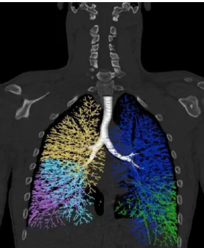
Figure 5: Space-filling tracheo-bronchial tree representation on a human lung. The tree is built by propagating the first segmented airways into the segmented lobes in order to fill their envelope. Constructed branches are modeled as pipes with radius and length determined by the algorithm depicted in [32]. Each of the five colors corresponds to a lobe.
4.2. Mesh generation from DICOM MRI image
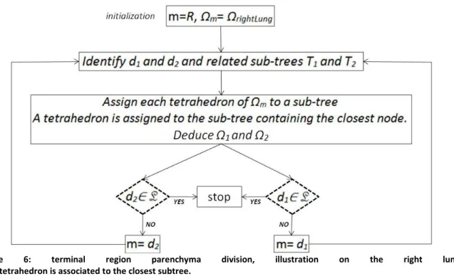
To generate a mesh for the finite element solver, we use HRCT DICOM data from [31]. DICOM images are first treated with Matlab to generate a surface triangle mesh. This surface mesh is then processed with Meshlab software [33]. First we perform decimation to adjust the mesh size as desired, then smoothing through a Taubin filter [34] to improve mesh quality. We use Gmsh [35] to generate from the surface mesh a 3D tetrahedric volume mesh. Once the 3D mesh is built, each tetrahedron is assigned to one of the tree exits according to the algorithm described in Figure 6. We denote by m a mother branch, m a region of the parenchyma fed by m, d1 and d2 the daughter
branches of m, 1 and 2 the regions of the parenchyma fed respectively by d1 and d2, T1 and T2 the
subsets of the tracheo-bronchial tree fed respectively by d1 and d2, R and L the daughters of the
trachea and L the list of the chosen tree exit branches: L={
ex
i}. So-called nodes are the bifurcation17
Figure 6: terminal region parenchyma division, illustration on the right lung.
Each tetrahedron is associated to the closest subtree.
As stated in 2.1, the chosen exits are not necessarily the conductive tree terminal branches. Figure 7 illustrates the process on a schematic tree with 3 chosen exits exi.
Figure 7: illustration of the subdivision process for a three exit tree defining three terminal regions. Each bifurcation gives birth to two subtrees. Each elementary volume of the domain is fed by gas flowing through this bifurcation is assigned to the subtree containing the closest node.
Figure 8 illustrates a lobar subdivision on a physiological geometry. The subdivision is built upon a 12 generation tree with 1633 exits.
18
Figure 8: illustration of a lobar subdivision on a physiological geometry. Segmented upper airways are represented along with the lung mesh subdivided at the lobar level. Lobe nomenclature is: LU=Left Upper lobe, LL=Left Lower lobe, RU=Right Upper lobe, RM=Right Middle lobe, RL=Right Lower lobe
Remark 5: Code vectorization makes the process fast. On aZBook15, IntelCoreTM i7-4810MQ
[email protected]*8 it takes less than one minute to subdivide a 51495 tetrahedrons mesh for a 12 generation conductive tree with 1633 exits.
4.3. Surface displacement registration
To impose Dirichlet boundary conditions, we need to have the displacement field of the surface over time. To that end we used Deformetrica software [36] that performs non-linear surface registration on surface meshes via the currents method [37]. This computed displacement is not physical in the sense that no mechanics is included in the underlying process. Since there is no uniqueness in surface points correspondence from one inflation state to another this may lead to non-physiological evolution. Yet Deformetrica allows the addition of landmarks and curves correspondence to the process so that physiological patterns can be tracked along the breathing cycle. Doing so provides registration with a more physical basis.
In the following section results of simulations performed on the tree-parenchyma coupling and the exit compartment models are presented.
5. Simulations and results
Simulations have been performed using a human lung geometry acquired in the supine position [31]. In [31] MLV (Mean Lung Volume) HRCT scan of the parenchyma envelope are provided along with lobar and upper airways segmentation. In what follows MLV is taken as the reference zero stress configuration. Applying processes described in 4.1, we build a space-filling tree within the MLV geometry. For both right and left lungs at MLV we build 3D meshes sub-divided from the generation ten level (see 4.2). The left lung mesh contains 51495 tetrahedrons distributed in 477 terminal regions. The right lung mesh contains 43395 tetrahedrons distributed in 752 terminal regions. Mechanical properties are assumed to be homogeneous. They are chosen following ranges provided in [38]: Young’s modulus E=1.256.103Pa, Poisson ratio =0.4, parenchyma density =100kg/m3. MLV volume is 2.231L. Following (24) we compute the equivalent static compliance C=2.10-6m3/Pa. Gravity
19 is neglected. Lobe nomenclature is: LU=Left Upper Lobe, LL=Left Lower, RU=Right Upper Lobe, RM=Right Middle Lobe, RL=Right Lower Lobe.
In the following we investigate the tree-parenchyma coupled model. The impact of using non-linear resistances vs. linear ones is studied in both healthy and pathological configurations. Then we test the mechanical independence assumptions associated with the exit-compartment model. Applying the process described in 2.4, we show how the tree-parenchyma model can generate appropriate forcing terms for the exit compartment model. In a following section we compare experimental lobar ventilation with simulation results obtained when applying Dirichlet boundary conditions built from imaging. Results obtained with the Dirichlet boundary conditions and with homogeneous Neumann pressure boundary conditions are compared in order to investigate the effect of boundary conditions spatial heterogeneity on ventilation. Finally we present a pressure controlled mechanical ventilation simulation for which non-linear Robin boundary conditions (see 3.1) are implemented.
In the following we usually display relative volume expansion from the reference state, displacement maps, and pressure maps where pressure is defined as:
(33)
with notations defined in section 2.2 and 2.4.
5.1. Tree-parenchyma coupled model
In this section we investigate the tree-parenchyma coupled model described in 3.1. We simulate spontaneous tidal breathing driven by Neumann homogeneous pressure boundary conditions, first in a healthy configuration, then in the case of a bronchoconstriction.
Linear (1) and non-linear (2) resistance models are compared. There is no consensus on the spatio-temporal pleural pressure profile during the breathing cycle [27]. In this section we impose an academic piecewise constant pressure pattern with a physiological plateau of
at inspiration [27] and at expiration so as to simulate passive recoil. This approach isolates the effect of the tree resistance distribution by ensuring that simulated ventilation heterogeneities are not due to spatial heterogeneities in the boundary conditions.
In Figure 9 left lung lobar volumes are plotted. Branch resistances are computed with the Poiseuille resistance model. The time step is .
20
Figure 9: left lung lobar volume expansion evolution from the reference state in a healthy configuration. A piecewise constant in time, homogeneous pressure profile is imposed as boundary condition. Resistances are computed with the Poiseuille theory.
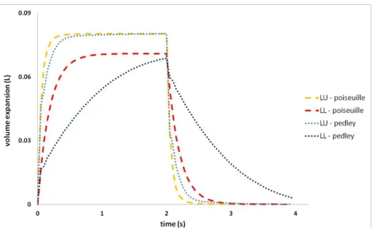
Let us first note that with a physiological pleural pressure amplitude, we obtain physiological volume amplitudes. In the frame of tidal breathing, linear elasticity thus seems to be a reasonable approximation. Both volume lobes evolve in phase with the applied pressure, and the tree resistance induces a time delay in the system’s response. Ventilation distribution is proportional to the reference state lobar volumes. In Figure 10 we compare Poiseuille, Pedley and a zero resistance tree configuration.
Figure 10: LU lobe volume expansion from the reference state in a healthy configuration. Comparison of Poiseuille, Pedley, and zero resistance models.
Since it takes into account pressure drops at bifurcations, the Pedley model results in higher resistances than the Poiseuille model. With higher resistance the dissipation within the system increases, in turn inducing a longer time delay. The higher the resistance, the higher the dissipation and consequently the lower the expansion generated for a given applied pressure. Here, the time delay is underestimated since tissue viscosity and the extra-thoracic contribution to the pressure drops are not considered. Note also that measured airway resistances show a high variability among individual, from 0.5 to 2.5 cmH2O.L-1.s-1 [39], inducing a variability of response times. The lung slice plot in Figure 11 shows the spatial distribution at time (inspiration) of the relative volume variation and the magnitude of the effective pressure field.
21
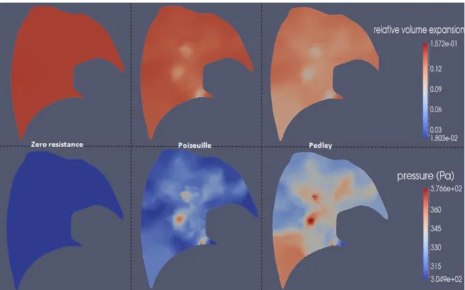
Figure 11: relative volume expansion from the reference state and effective pressure (33) magnitude maps on a left lung slice. The homogeneous constant piecewise pressure shown in Figure 10 is applied around the parenchyma. Comparison at time 0.25 s in a healthy configuration for different airway resistance models: zero resistance, Poiseuille and Pedley.
As described in section 2.4, the effective pressure field within the parenchyma is made of two components: the elastic pressure due to expansion and the pressure drop within the tree. The higher the pressure drop through this path, the higher is in the region. The coupling pressure opposes volume variations; thus regions fed by a path along which pressure drop is high,
expand less during inspiration and contract less during expiration. In inspiration the elastic pressure is thus reduced. The behavior of is a balance between the elastic and the coupling
pressure. At a time in the breathing cycle when flow is high, pressure drops along the tree are increased and the increase of the coupling pressure compensates the decrease of the elastic pressure. Regions fed by a higher resistive path expand less. This is what is observed in Figure 11 : the effective pressure and the volume expansion maps are anti-correlated. Moreover, Pedley resistances are higher than Poiseuille’s. Thus, the effective pressure map is more heterogeneous. When the tree resistances are set to zero, the effective pressure reduces to the elastic pressure. The latter is homogeneous since a homogeneous pleural pressure is applied around the parenchyma. Note that at times of the breathing cycle when the flow is lower, pressure drops are reduced and the effective pressure maps would be then more homogeneous.
Next we simulate a bronchoconstriction of the branch feeding lobe LL by reducing its diameter by a factor of 5. We compare the resulting lobar volume evolutions obtained using the Poiseuille and Pedley models as shown in Figure 12.
22
Figure 12: left lung lobar volume evolution with a bronchoconstriction simulated on the branch feeding lobe LL. Comparison of Poiseuille and Pedley resistance models.
A diameter reduction induces a resistance increase. Poiseuille and Pedley models exhibit notable differences showing that resistance non-linearities have to be taken into account when modeling ventilation distribution in pathological situations. Again, we observe an increasing phase shift with higher resistances. This is consistent with other studies [40]. Compared to the healthy configuration, ventilation of lobe LL is logically reduced: the driving effort is constant while the energy necessary to induce flow through the bronchoconstricted branch increases. Again, volume expansion and effective pressure are anti-correlated (see Figure 13).
Figure 13: relative volume expansion from the reference state and effective pressure (33) magnitude mapson a left lung slice. The homogeneous constant piecewise pressure shown in Figure 10 is applied around the parenchyma. A uniform diameter reduction of factor 5 is applied to the branch feeding lobe LL. Comparison at time 0.25 s for Poiseuille and Pedley resistance models. The dashed line represents the lobar frontier.
23
5.2. Mechanical independence in the exit compartment model
In the exit compartment framework, terminal compartments are mechanically independent. This may not properly describe the continuum nature of the parenchyma. Here we simulate pulmonary fibrosis and compare results from both models. To mimic tissue stiffening associated with this pathology, the Young’s modulus of lobe LL is divided by ten. Equivalently, compliances of exit compartments belonging to lobe LL are divided by ten. Resistances are computed with Pedley’s model (2). A homogeneous smoothed piecewise constant in time pressure is applied to both models. Lobar volume evolution of the left lung is plotted in Figure 14.
Figure 14: left lung lobar volume evolution from the reference state, fibrosis simulated on lobe LL. Comparison of the tree-parenchyma coupling and the exit-compartment models.
Lobe LL is indeed less ventilated in both models. In the exit-compartment framework no mechanical connection exists between both lobes. LU is not affected by fibrosis while in the tree-parenchyma coupling case LU ventilation is slightly reduced, but lobar ventilation shows little difference. Effects are mainly local as demonstrated in Figure 15 and Figure 16.
Figure 15: relative volume expansion on a left lung slice, from basis to apex. The homogeneous piecewise constant pressure shown in Figure 10 is applied around the parenchyma. The map is shown at time 0.5 s.
24 tree-parenchyma coupled model. As expected the expansion of the diseased lobe is reduced compared to the healthy one, stiffening makes volume change harder. We note that, due to the mechanical interaction between both lobes, LU regions next to LL are affected by fibrosis although their mechanical properties are unchanged.
For the 477 terminal regions of the left lung, we plot the expansion ratios defined as
for both exit-compartment and tree-parenchyma coupled models at t=0.5s.
Figure 16: Expansion ratios of the left lung 477 terminal regions at a given lung expansion for the exit-compartment and the tree-parenchyma coupled models. Simulations are performed with homogeneous pressure boundary conditions. To simulate fibrosis, lobe LL compliance (resp. Young's modulus) was divided by ten.
In the exit compartment framework, expansion ratios are uniform in each lobe. The healthy lobe behavior is independent of the diseased region and . Since compliance is divided by ten in the fibrosed lobe LL, expansion ratios are uniformly divided by ten: . This demonstrates the mechanical independence of terminal regions in the exit compartment framework. As observed in Figure 15, regions do mechanically interact in the tree-parenchyma coupling framework. Some regions of lobe LU expand less when LL is fibrosed because they are affected by the stiffening of neighboring areas. Some regions of LL expand more than in the exit compartment model because they are pulled by neighboring healthy areas. From this result and other pathological simulations (results not shown here: healthy configuration, bronchoconstriction on one branch, regional bronchoconstriction) we conclude that taking into account the mechanical interaction between regions does impact the ventilation distribution.
25
exit-compartment model
We showed in section 5.2 a possible limitation associated with exit-compartment models. In 2.4 a method to compute applied forces for the exit-compartment model based on the tree-parenchyma coupled model simulations has been described. We apply this approach to the case presented in section 5.2. Simulating pulmonary fibrosis as in 5.2 we get
Figure 17: Expansion ratios of the left lung 477 terminal regions at a given lung expansion for the tree-parenchyma coupled model with homogeneous pressure boundary conditions and the exit compartment model with equivalent boundary conditions. To simulate fibrosis, lobe LL compliance (resp. Young's modulus) is divided by ten.
We recover the same ventilation distribution in both cases. Here, the pressure applied around the parenchyma in the tree-parenchyma coupled model is homogeneous. In order to recover the same ventilation results in the exit-compartment model this pressure has to be heterogeneously distributed such that it accounts for the mechanical interaction between terminal regions. Yet, as shown in the next section, the pressure around the parenchyma itself is heterogeneous when applying Dirichlet boundary conditions coming from image registration.
5.4. Dirichlet Boundary conditions registered from medical images
In this section we reconstruct the lung parenchyma surface evolution based on HRCT data provided by [31]. It can be applied as boundary condition to our finite element model.
5.4.1. Impact of boundary conditions on lung regional expansion
In addition to MLV data, [31] provides TLC HRCT scans of the lung envelope along with lobar segmentation. Following 4.3 we perform non-linear surface registration from the MLV to the TLC state. Physiological landmarks and surface lobe fissures (see appendix 8.2) can be included in the segmentation process (see Figure 18).
26
Figure 18: from MLV to TLC with landmarks and lobe fissures – illustration on an imaged right lung
In what follows we assume MLV to be the reference state. Here imaging measurements are static. Thus we do not consider any dynamics in the transition from MLV to TLC, and airway resistances are set to zero. The registered displacement field is used as a Dirichlet boundary condition.
In Figure 19 we compare experimental lobar ventilation ratios (issued from image segmentation) with results obtained from the model in three cases: surface displacement field registered without landmarks or lobe fissures, with landmarks only (10 on the left lung surface, 16 on the right one), and with both landmarks and lobar fissures.
Figure 19: lobar ventilation distribution, simulation vs. experimental data. Experimental data are deduced from lobar segmentations on CT images at the two inflation states. Simulations are carried out with Dirichlet boundary conditions issued from image registration. Three registered surface displacement fields are used: crude registration performed without landmarks or lobar fissures, registration performed with landmarks, and registration performed with both landmarks and lobar fissures.
As we add physiological information to the registration process, results get more accurate. Whether landmarks or fissures contribute more to the improvement depends on the number of landmarks used and on their relevance. Here adding landmarks to the process improves the result by 7% on
27 average. Adding fissures brings a further 2% improvement. The residual error can have several sources: here we neglect the lobe sliding, though it may affect the parenchyma displacement field [41]. The volume increase from MLV to TLC is about 70%: intermediary states images between the two configurations would ensure a better registration and hence more accuracy in ventilation prediction. Linear elasticity is a rough approximation for large displacements. With this constitutive relation, recoil effort is increasingly underestimated as the parenchyma expands. Displacement may be well predicted but a proper effort computation requires an appropriate mechanical law for the parenchyma. Despite these strong assumptions, results are encouraging. This shows that surface parenchyma displacement field is an appropriate boundary condition when it comes to lung ventilation modeling. This points out also how crucial it is for the registration to be precise. If 4DCT [42] or 4D-MRI [43] data along with segmented upper airways were available in a pathological case where tree resistance is increased, it would be of great interest to run the model with dynamic Dirichlet boundary conditions and to compare the resulting simulation to the corresponding dynamic ventilation acquisition; depending on the tree resistance distribution the tree-parenchyma coupling could then be emphasized.
Moreover, it has been widely assumed that esophageal pressure can be used as a surrogate for pleural pressure [27]. However, esophageal pressure is a scalar that cannot account for spatial heterogeneity. Some studies have applied a homogeneous pressure as the boundary condition [7], [44]. In [6] a pressure gradient is applied to account for gravity effects. In this section, we investigate how heterogeneities in boundary conditions impact ventilation distribution. As a post-process of the ventilation distribution simulation (Figure 19) we can compute the equivalent average normal time varying effort (notations defined in section 2.4) and apply it as a forcing term for comparison.
Figure 20: left lung lobar distribution at TLC state obtained with Dirichlet boundary conditions issued from image registration vs. homogeneous pressure boundary conditions.
In the framework of linear elasticity, when a homogeneous pressure is applied and tree resistances are set to zero, the ventilation of a region is proportional to its volume. Thus lobe LU expands more than LL because it is bigger. With Dirichlet boundary conditions issued from imaging, LL is more ventilated because the diaphragm has a larger contribution to parenchyma expansion than the ribs. In Figure 21 we plot the displacement field magnitude on a lung slice obtained with the two previous boundary conditions at a given volume expansion.
28
Figure 21: magnitude displacement field on a left lung slice. On the left, homogeneous pressure boundary conditions are applied; on the right Dirichlet boundary conditions issued from imaging are applied.
The displacement magnitude is much more heterogeneous with the Dirichlet boundary conditions registered from images than with homogeneous pressure boundary conditions. The parenchyma is more stretched at the base, where the diaphragm pulls, than at the apex.
Boundary conditions have a crucial impact on ventilation. This points out the need to take into account their heterogeneities when modeling ventilation. Here tree resistances have been set to zero. Imposing a displacement field while increasing some branch resistances in the tree because of pathological patterns could lead to more heterogeneities.
5.4.2. Tree-parenchyma coupled model with Dirichlet boundary conditions
The displacement field built in previous section maps the MLV to the TLC configuration. To generate a tidal look alike breathing pattern, we bound it and impose a sinusoidal dynamics with four seconds time period (see Figure 22). The overall relative volume amplitude from the reference state is 22%.
29
Figure 22: left lung and lobar volume evolutions from the reference state in a healthy configuration. Dirichlet boundary conditions with sinusoidal time evolution are applied. Resistances are computed with the Pedley resistance model.
We compare the ventilation (Figure 23) and (Figure 24) distributions obtained in a healthy case and when a bronchoconstriction with ratio 7 is applied on the branch feeding lobe LU.
Figure 23: Relative volume expansion 3D map on a left lung geometry. Dirichlet boundary conditions with sinusoidal time evolution are applied. Resistances are computed with the Pedley resistance model. On the left side a healthy configuration is simulated, on the right side a bronchonconstriction with ratio 7 on the branch feeding lobe LU is applied. Plot at time t=3s.
As noted in 5.4.1, volume distribution is heterogeneous. In the pathological case, lobe LU expands less than in the healthy situation. Here applied boundary conditions prescribe the lung total volume evolution, so lobe LU reduced ventilation of is associated with an increased expansion of lobe LL.
30
Figure 24 : effective pressure (33) magnitude map on a left lung geometry. Dirichlet boundary conditions with sinusoidal time evolution are applied. Resistances are computed with the Pedley resistance model. On the left side a healthy configuration is simulated, on the right side a bronchonconstriction with ratio 7 on the branch feeding lobe LU is applied. Plot at time t=3s.
The effective pressure magnitude is higher next to the diaphragm than near the apex. As lobe LU is harder to expand, the pressure applied to generate a prescribed volume expansion is greatly increased in that region.
5.5. Pressure controlled mechanical ventilation
In this section, a pressure controlled mechanical ventilation scenario is simulated on the left lung. The system is governed by (32) . As depicted in 2.2, chest and diaphragm resistance to lung expansion are modeled through non-linear Robin boundary conditions that prevent lobes from expanding over their TLC volume. Segmented lobe volumes at TLC are taken from [31]. In this scenario, the ventilator pressure increases till both lobes are maximally expanded and then suddenly drops to zero (see Figure 25). This is not a clinically realistic pattern. The simulation rather aims at validating the Robin boundary conditions. To isolate the effect of the imposed boundary conditions, tree resistances are set to zero. Chosen parameters for the simulation (defined in 3.1) are: , tol=0.02, stepMin=0.001, stepMax=0.5, nbItS=30, i ci=1 (20).
31
Figure 25: Pressure controlled mechanical ventilation – lobar volume expansion from the reference sate. Maximum expansion is the TLC.
Lobar volumes achieve and remain at their maximum values. It takes more pressure to saturate LL than LU. The reason is that the relative difference between MLV and TLC volume states is higher for LL. When zero pressure is applied, the system instantaneously goes back to the equilibrium position. This is coherent with the facts that inertia is negligible and tree resistances are set to zero.
Remark 6: As in Erreur ! Source du renvoi introuvable. the linear elasticity assumption does not hold
true for large displacements. Taking lobe sliding into account may change the required effort to reach TLC. Here the Robin function is homogeneous at the lobar level; it should be heterogeneous in order to account for real efforts which are probably heterogeneous since the ribs and diaphragm have specific actions on the parenchyma [45].
5.6. Computation time
Both the exit compartment and tree-parenchyma coupled models are implemented in an efficient way. In the exit compartment case, matrix-vector product and matrix inversion are performed without operator storage. This is made possible by the dyadic property of the tree [24]. In the tree-parenchyma coupling case we also take advantage of the tree structure to compute matrix-vector product without storing the full coupling matrix (see 3.1). Simulations are run on a single processor of ZBook15, IntelCoreTM i7-4810MQ [email protected]*8. The simulation shown in Figure 10 takes 279 s (CPU time) for eighty time steps on a 51495 tetrahedrons mesh, the equivalent simulation with the exit-compartment model takes 15 s (CPU time) for a 1229 exits tree.
6. Conclusion
In conclusion, we have built a computationally efficient mechanical model of the lung in which the tracheo-bronchial tree and parenchyma are coupled. It gives relevant and promising results. Simulations performed on a 477 exits tree took a few seconds per time step. The results pointed out the importance of nonlinearities in the airway tree for pathological conditions. Furthermore, we addressed the crucial question of boundary conditions. Applying Dirichlet boundary conditions based
32 on parenchyma surface registration proves to generate good results in comparison with experiments. We also investigated limitations inherent to the exit compartment models. Both the lack of information on the pleural pressure spatio-temporal heterogeneity and the mechanical independence of the compartments can lead to inaccurate ventilation predictions. To overcome these drawbacks, we proposed a method to compute pressure boundary conditions that includes mechanical interaction between compartments and surface displacement patterns and which, applied to the exit-compartment model, provided good ventilation results. Our framework is able to deal with pressure, surface displacement and also nonlinear Robin boundary conditions. We can thus model mechanical ventilation with constraints on the boundary that ensure lung volumes cannot expand over TLC.
Future work would include a more realistic non-linear constitutive relation for the parenchyma along with a study of the effect of gravity on ventilation. An experimental validation of the tree-parenchyma coupling could be performed based on dynamic tree-parenchyma CT acquisition.
7. Acknowledgements
This work was supported by an ANR grant (ANR-11-TECS-006). Nicolas Pozin was funded by ANRT through a CIFRE thesis INRIA-Air Liquide Santé International. Authors gratefully acknowledge Mr. Fabien Raphel and Mrs. Cécile Dubau for their great support with implementation.
8. Appendix
8.1. On assuming flow into the mother branch equals the sum of the flows
entering the daughters
Some studies [7], [13] include compliant airways in the tree model following the description given in Figure 26. Airway compliance is given by
with and where k1=-0.0057 mm-1, k2=0.2096, k3=0.0904mm.
Figure 26: resistive compliant airway model.
In Figure 26, is the flow entering the airway, is the instantaneous volume variation per unit
time of the airway, is the flow leaving the airway and is the pressure in the parenchyma
region surrounding the branch. Assuming, as in [7], that is constant, we can write
and . We have . Formulas (3) and (4) are valid only if the flow going
through an airway equals the flow going through its daughters; this requires , which
means airways are close to rigid. In the following we investigate the validity of this assumption on the model given by Figure 27.
Let us compute the order of magnitude of the flow at each generation using a rigid-tree model. To get general insights of the flows in the tracheo-bronchial tree, we work on simple models such as a purely symmetrical Weibel tree representation [20]. In this model flows equally distribute at every