Coordinate-independent computations on differential equations

(1)

Coordinate-Independent Computations

on Differential Equations

by

Kevin K. Lin

Submitted to the Department of Electrical Engineering and Computer Science in partial fulfillment of the requirements for the degree of

Master of Engineering in Electrical Engineering and Computer Science at the

MASSACHUSETTS INSTITUTE OF TECHNOLOGY August 11, 1997

@

Author ...

Department of Electrical Engineering and Computer Science August 11, 1997

Certified by ... ...

Gerald Jay Sussman Matsushita Professor of Electrical Engineering Thesis Supervisor

Accepted by... ... " " ... .. ... ... ... A. C. Smith Chairman, Department Committee on GradbRte Theses

MA SACHUS IN TITUL OF TECHNOLOGY

JUL

14 19q8

(2)

Coordinate-Independent Computations on Differential Equations

by

Kevin K. Lin

Submitted to the Department of Electrical Engineering and Computer Science on August 11, 1997, in partial fulfillment of the

requirements for the degree of

Master of Engineering in Electrical Engineering and Computer Science

Abstract

This project investigates the computational representation of differentiable manifolds and the use of such abstractions to help manage multiple coordinate systems on n-dimensional spaces. This idea is applied to the accurate integration of ordinary differential equations using multiple coordinate systems. An attempt is also made to apply this idea to the numerical solution of linear partial differential equations, although in this case unexpected difficulties arise even with the simplest equations.

Thesis Supervisor: Gerald Jay Sussman

(3)

Acknowledgments

As is the case with any undertaking, there are far too many people to thank in relation to this project. If I neglected anyone, it is purely out of failure of memory and I beg for their forgiveness.

To begin, I would like to thank Norman K. Yeh and Mariya Minkova for proof-reading my thesis proposal, and Tim McNerney for suggestions on how to present manifolds. Because of them, the presentation is much better than the rambling mess that was my first draft.

To the folk at Switzerland, especially Daniel Coore and Jim McBride: Thanks for the stimulating (and sometimes late-night) discussions on life, the universe, and everything. Thanks are also due to Eric Grimson, Thanos Siapas, and Ken Yip for crucial references, to Hardy Mayer and Michael Chechelnitsky for many helpful conversations on PDEs, and to Rebecca Bisbee and Anne Hunter for making sure that all the important things got done.

Portions of this work was supported by the Barry M. Goldwater Foundation, without whose help it would have been difficult to get this far.

I am forever indebted to my teachers throughout the years: To Mr. Reyerson at BCP, and Professors Flanigan and Morris at SJSU, for introducing me to mathematics; to Pro-fessors Munkres, Guillemin, and Wisdom for being such great teachers; and finally, to Gerald Jay Sussman, who has helped shape my interests, guided my work, and above all else encouraged me onward as I took the first faltering steps into a world of breathtaking wonders.

To my family and all my friends: You have made a great difference, and I could not have made it without you.

Still round the corner there may wait A new road or a secret gate;

And though I oft have passed them by, A day will come at last when I

Shall take the hidden paths that run West of the Moon, East of the Sun. -J. R. R. Tolkien

(4)

To Grandpa.

(5)

3.4.5 Basic FEM algorithm on manifolds . . . . 3.4.6 Interpolation between charts . . . . 3.4.7 Some numerical results . . . . 3.4.8 The problem with interpolation . . . . 3.4.9 Other approaches to FEM on manifolds . . . . 3.5 Some comments on mesh generation . . . . 3.6 Directions for future work ...

3.6.1 Improvements to finite differences . . . . 3.6.2 Improvements to finite elements . . . . 3.6.3 Other methods ...

4 Problems with Time

4.1 The linear wave equation . . . . 4.2 Initial value problems and characteristics . . . . 4.2.1 Characteristic curves for a first-order equation . . 4.2.2 Characteristics for general equations . . . . 4.2.3 Variational principles revisited . . . . 4.2.4 Galerkin's method and the initial value problem 4.3 Variations on a theme of Lagrange . . . .

4.3.1 Modifying the action principle . . . . 4.3.2 Modifying the domain . . . . 4.4 Difficulties with the spacetime approach . . . . 4.4.1 Why the variations failed . . . . 4.4.2 Other problems ...

4.5 Directions for future work ...

A Background Material on Partial Differential Equations A.1 Matrix inversion ...

A.1.1 Iterative methods and relaxation . . . . A.1.2 Jacobi iteration...

A.1.3 Gauss-Seidel iteration . . . .

74 75 80 83 83 89 92 98 ... . 101 106 ... . 117 118 118 ... . 119 .... 119 120 121 122 .. 123 124 .. 125 .. 127 .. 128 .. 128 .. 135 .. 140 .. 140 141 142 143 ... 143 . 143 ... 144 . 145 A.1.4 Overrelaxation ... 145

(7)

A.2 A brief introduction to finite elements A.2.1 Introduction ...

A.2.2 Partial differential equations A.2.3 The Rayleigh-Ritz Method A.2.4 Galerkin's method . . . .

B Odds & Ends

B.1 Charts without a manifold ...

B.2 Integration of differential forms on oriented manifolds B.2.1 Stokes's theorem

C Complete Program Listings C.1 Computational manifolds C.1.1 basis-imb.scm . . . C.1.2 basis-poly.scm... C.1.3 basis-real.scm . . . C.1.4 boundary.scm... C.1.5 bug.scm ... C.1.6 charts.scm... C.1.7 cotangent.scm... C.1.8 fields.scm ... C.1.9 hamilton.scm ... C.1.10 imbedding.scm . . C.1.11 job-ode.scm .... C.1.12 job-pde.scm .... C.1.13 lagrange.scm . . . C.1.14 linear.scm ... C.1.15 load-main.scm C.1.16 load-ode.scm . . . C.1.17 load-pde.scm . . . C.1.18 lshared.scm .... C.1.19 manifold.scm . .. C.1.20 misc-math.scm . . C.1.21 misc.scm... C.1.22 ode-examples.scm C.1.23 ode-fast.scm .... C.1.24 ode.scm ... . . . . . 145 . . . . 145 . . . . . . . . . . . . 146 148 153 155 155 156 157 158 158 158 160 162 163 167 167 169 173 179 179 180 181 182 184 187 187 188 189 192 197 197 199 203 204 .. .. .. .. .. . .. .. .. . . .

(8)

C.1.25 pde-aux.scm . C.1.26 pde-charts.scm .. C.1.27 pde-cmpgrd.scm C.1.28 pde-collect.scm . C.1.29 pde-collectl.scm C.1.30 pde-collect2.scm C.1.31 pde-collect3.scm C.1.32 pde-collect4.scm C.1.33 pde-config.scm .. C.1.34 pde-debug.scm .. C.1.35 pde-elements.scm . C.1.36 pde-examples.scm C.1.37 pde-gentest.scm.. C.1.38 pde-main.scm . . . C.1.39 pde-mergers.scm C.1.40 pde-nodes.scm .. C.1.41 pde-ops.scm.... C.1.42 pde-test.scm . . C.1.43 pde-thesis.scm C.1.44 pde-thesisl.scm. C.1.45 pde-thesis2.scm C.1.46 pde-thesis3.scm C.1.47 pde-thesis4.scm . C.1.48 pde-tools.scm .. . C.1.49 pde-works.scm .. C.1.50 product.scm.... C.1.51 ranges.scm .... C.1.52 richardson.scm .. C.1.53 rigid-body.scm .. C.1.54 rigid-compute.scm C.1.55 rigid-errors.scm. C.1.56 rigid-fields.scm .. C.1.57 rigid-read.scm... C.1.58 rigid-test.scm . . C.1.59 rigid-too.scm .. . C.1.60 rigid-tops.scm... C.1.61 rigid.scm ... .. . .. .. . .. .. .. .. .. . .. . 209 . . . . 210 . .. . .. .. .. .. . .. .. .. .. . 213 . . . . 219 ... . .. . .. .. .. .. .. .. .. . 220 ... . .. . .. .. . .. ... . .. .. 220 . . . . 221 . . . . 221 . . . . . 222 . . . . . 222 ... . . . . 232 . . . . . 233 ... . . . . 235 . . . 236 . . . . 244 . . . 249 . . . . 251 . . . . 252 . . . . 255 . . . . 256 . . . . 257 . . . . 258 . . . . 258 . . . . 259 . . . . 263 . . . . 265 . . . . 267 . . . . 269 . . . . 271 . . . . . 274 . . . . 274 . . . . 275 . . . . 282 . . . . 283 . . . . 284 . . . . 286 . . . . 287

(9)

C.1.63 spaces.scm ... 298 C.1.64 stubs.scm ... 306 C.1.65 tangent.scm ... 307 C.1.66 vbundle.scm ... 312 C.2 Finite elements ... 314 C.2.1 2d-domains.scm ... 314 C.2.2 2d-examples.scm ... 323 C.2.3 2d-operators.scm ... 326 C.2.4 2d-poly-basis.scm ... 328 C.2.5 2d-real-basis.scm ... 333 C.2.6 2d-real-diff.scm ... 334 C.2.7 2d-trapezoid.scm ... 335 C.2.8 basis.scm ... 336 C.2.9 bent.scm ... 338 C.2.10 collect.scm ... 340 C.2.11 debug.scm ... 341 C.2.12 delaunay.scm ... 346 C.2.13 delaux.scm ... 349 C.2.14 dyntable.scm ... 351 C.2.15 edge.scm ... 352 C.2.16 fem .scm ... 356 C.2.17 job.scm ... 362 C.2.18 jobl.scm ... 362 C.2.19 load.scm ... 363 C.2.20 matlib.scm ... 363 C.2.21 nodes.scm ... 371 C.2.22 opalg.scm ... 372 C.2.23 operators.scm ... 373 C.2.24 relax.scm ... 374 C.2.25 sparse.scm ... ... 375 C.2.26 thesis.scm ... 378 C.2.27 thesisl.scm ... 379 C.2.28 util-too.scm ... 379 C.2.29 util.scm ... 381 C.3 Finite differences ... 382 C.3.1 farray.h ... ... 382 C.1.62 smooth.scm 293

(10)

C.3.2 gunk.h... C.3.3 matrix.h ... C.3.4 random.h . . . . C.3.5 stat.h ... C.3.6 accum.c . . . . C.3.7 approx.c ... C.3.8 band.c... C.3.9 blud.c ... C.3.10 check.c ... C.3.11 circle.c ... C.3.12 dot.c... C.3.13 estimate.c . . . . C.3.14 farray.c ... C.3.15 femcompact.c ... C.3.16 femstats.c ... C.3.17 fill.c ... C.3.18 filt.c ... C.3.19 grad.c ... C.3.20 gsmat.c . . . . C.3.21 gsort.c . . . . C.3.22 gunk.c . . . . C.3.23 gunk2mat.c ... C.3.24 hilbert.c . . . . C.3.25 improve.c ... C.3.26 jacmat.c . . . . C.3.27 list2grid.c ... C.3.28 lud.c... C.3.29 maplegrid.c ... C.3.30 matrix.c . . . . C.3.31 migrate.c . . . . C.3.32 mkbd.c ... C.3.33 mkgrid.c ... C.3.34 mksq.c... C.3.35 new2old.c ... C.3.36 normeqs.c . . . . C.3.37 nstat.c... C.3.38 old2new.c ... 382 384 384 385 385 388 395 396 402 404 406 411 413 414 415 416 417 419 420 423 425 432 434 435 439 442 443 446 447 453 456 460 461 465 466 475 475

(11)

C.3.40 peek.c ... 477 C.3.41 peekcoeff.c ... 480 C.3.42 poly.c ... 483 C.3.43 pot.c . . .. . . . .. . .. . . . 489 C.3.44 random.c ... 489 C.3.45 relax.c ... ... ... 490 C.3.46 repos.c . .. ... . . .. . .. . . .. . ... ... .. .. . .. . 493 C.3.47 reset_val.c ... 495 C.3.48 rref.c . . . 496 C.3.49 sam ple.c ... 497 C.3.50 scramble.c ... 501 C.3.51 slice.c . . . 502 C.3.52 spect.c . .. . .. .... . .. . .. . . .. ... ... . . . 504 C.3.53 sqstat.c ... ... 506 C.3.54 stat.c . . . .. . . . .. . . . 507 C.3.55 walk.c ... 509 C.3.39 order.c . 476

(12)

Chapter 1 Introduction

Partial differential equations1 arise naturally in a large variety of physical problems. Like or-dinary differential equations, the majority of partial differential equations cannot be solved analytically save in special cases. Thus, efficient and accurate numerical solutions of partial differential equations are essential in many applications. However, unlike ordinary differen-tial equations, the solution of even linear pardifferen-tial differendifferen-tial equations can be a non-trivial task. There are no general methods that apply to all types of partial differential equations,

and it is often necessary to exploit special structures in the problem at hand.

This project explores the the numerical solution of partial differential equations using coordinate-independent representations. This approach makes possible the use of whatever coordinate system that happens to simplify the problem locally. As a result, we can exploit the structure and locality of interaction inherent in many physical systems, which can provide more accurate solutions as well as insights into the physical and mathematical structure of problems. In addition, it may also help us reformulate such problems for distributed computers. This project focuses on low-order linear equations in low dimensions for which analytical solutions are available, so that we can check our numerical solutions.

The rest of this document is divided into three chapters and three appendices. The first chapter develops the idea of differentiable manifolds and other basic concepts from modern differential geometry, and applies these concepts directly to the representation and solution of ordinary differential equations, particularly those arising from classical mechanics. Next, partial differential equations are discussed; for simplicity, the discussion is restricted to simple scalar linear equations, such as Laplace's equation over regions in the plane. Finally, the coordinate-independent solution of equations involving time, such as the linear wave equation, is investigated; in this context, the spacetime representation of equations (rather than the traditional "space + time") seems most natural.

(13)

While the manifold abstraction works beautifully with ordinary differential equations, some unexpected difficulties arise when dealing with even the simplest partial differential equations. Thus, most of the methods described herein, with one notable exception, actually do not work all that well, and in some cases completely fail. Thus, there is much work to be done. However, given the limited scope and time scale of this thesis project, not all possible solutions to these problems can be adequately explored. It is hoped that these ideas can be explored more fully in the future.

Appendix A includes relevant background material on partial differential equations. In particular, it presents the numerical methods that form a basis for this project, as well as some important geometric and analytical properties of partial differential equations. Appendix B contains some material on the theory of manifolds that was not directly needed in the thesis, while Appendix C contains complete program listings.

The entire document, including the material on abstract manifolds, suppose only a strong background in linear algebra and advanced calculus; little familiarity with more advanced mathematics is assumed. Also, it is helpful, though not necessary, to be acquainted with classical mechanics in Chapter 2, and §4.3.1 presumes some acquaintance with the basic concepts of relativity.

Finally, a note about the presentation: Throughout this document, programs imple-menting the main ideas will be presented alongside the mathematics. This serves a few different purposes: First, because this project is fundamentally about computational tech-niques, it would not be complete without actual programs. Second, it is often the case that seeing something presented in different ways aids in understanding, especially in subjects involving a significant amount of abstraction. Furthermore, programming languages, by their very nature, force one to be as careful with the details as with the main concepts, something that math and physics texts sometimes neglect. The language chosen for this project is Scheme, a dialect of Lisp. The choice is primarily based on the exceptional ease and flexibility with which Scheme expresses mathematical concepts; good references for the language are [9] and [2].

(14)

Chapter 2 Ordinary Differential Equations

and Manifolds

This chapter describes the computational representation of manifolds, as well as their use in the formulation and numerical solution of ordinary differential equations. As motivat-ing examples for the main definitions, problems in classical mechanics are presented usmotivat-ing the manifold formalism. In following chapters, some ideas for integrating linear partial differential equations using multiple coordinate systems are treated.

For a good reference on advanced calculus as well as an elementary introduction to manifolds, Munkres [21] is excellent. Also, Guillemin and Pollack give a beautifully lucid exposition on the topology of manifolds [14]. A more technical and abstract treatment is given in Warner [28], and the classic by Arnol'd [4] presents manifolds in the context of classical mechanics-An approach followed closely in spirit (but only in spirit) in this chapter.

2.1 A brief introduction to manifolds

This section introduces the basic notions using a physical example, which will be revisited from time to time as new concepts are developed.

2.1.1 The spherical pendulum

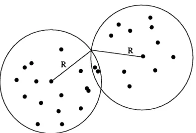
A good starting point for the study of manifolds is a variation on the classical pendulum, the spherical pendulum (see Figure 2-1): Suppose a point mass of mass m is connected to a fixed point by a massless rod of length 1. Furthermore, suppose that the point mass is allowed to move freely in any angle (not simply constrained to a vertical plane, as in the usual pendulum), and that it is subject only to a uniform gravitational field of constant

(15)

Figure 2-1: The spherical pendulum.

magnitude g.

The equations of motion for this problem are easy to derive. However, instead of de-riving the equations to analyze properties of the motion, let us focus on some of the more fundamental issues in a complete mathematical description of the problem. As we will see, this problem illustrates most of the basic ideas in the theory of manifolds.1

First, consider the problem of specifying the configuration of the system. What informa-tion do we need to specify the posiinforma-tion of the pendulum? Since the point mass is constrained to move at a constant distance I from the fulcrum, the problem of specifying configurations of the spherical pendulum is equivalent to the problem of locating points on a sphere.

In order to specify points on a sphere, there are a couple of alternatives. One natural idea is to use the fact that the two-dimensional sphere sits inside three-dimensional Euclidean space, and to use the coordinates of R3 to parametrize the sphere. Unfortunately, this approach is natural only for the sphere, and there are many important abstract spaces that cannot be easily visualized as subspaces of Euclidean space, such as the space of all orientations of a rigid body (which will be discussed later). Furthermore, in numerical integrations of ODEs, it will often happen that the trajectory "veers off" the sphere due to round-off error, and the constraint that the point mass lies at a constant distance I from the origin would no longer hold.

Another approach is to put coordinate systems on the sphere that require only two parameters. Formally, these are differentiable one-to-one mappings that map subsets of the sphere onto subsets of the plane and for which a differentiable inverse exists. This turns out

1

The ordinary pendulum, often used to illustrate important physical concepts, is not complicated enough geometrically to bring out the difficulties that manifolds were invented to handle.

(16)

to be a well-studied problem, since cartographers must deal with the fact that the surface of the Earth is spherical (approximately) but maps are fiat (Euclidean). The usual examples of map-making projections, such as the Mercator projection (cylindrical coordinates) or the system of longitudes and latitudes (spherical coordinates) are all examples of coordinate systems on the sphere. Note that there exists no two-parameter coordinate system that covers all of the sphere in a continuous fashion, but for every point on the sphere, we can always find a coordinate system that parametrizes a neighborhood of the point using a pair of parameters, so that the parametrization matches the dimension of the space.

In addition, in cartography, there is a natural solution to the problem that no coordinate system covers all of the Earth: We can simply use more than one map. We can simply switch to another map when one map becomes nearly useless. All that is required is some systematic way of figuring out when coordinates in two different maps are in fact the same point on the sphere, so that one could switch between maps without getting lost. This idea has been generalized beyond recognition to form the foundation of modern differential geometry, and spaces covered by maps (usually called charts) that make the space look "locally Euclidean" are called manifolds.

2.1.2 Differentiable manifolds

These ideas can be formulated mathematically as follows: Let M be a non-empty set of

points,2 and let n be some fixed positive integer. An n-dimensional chart on M is a triple

(U, V, q), where U is a subset of M, V an open subset of Rn, and 4 a one-to-one map of

U onto V (see Figure 2-2). 0 is a coordinate map, and a chart (U, V, q) is said to contain

a point p E M if U contains p. Given two charts C1 = (UI,Vi, 01) and C2 = (2, V2, 2),

suppose the intersection U1 n U2 is non-empty, and let Wi be the image ¢i(U1 n U2) for i = 1, 2. We can then form a transition map, 02 0-11, o which is a bijective mapping from

W1 to W2. Note that the inverse of this transition map is 41 o 4021, which is represented by

the same set of lines in Figure 2-2 with the arrows reversed. Now, if W1 and W2 are both

open subsets of Euclidean n-space, then it makes sense to talk about the differentiability of the transition map 02 o 0-1, and the charts C₁and C2 are said to be compatible if W1 and

W2 are open and the corresponding transition map is smooth, i.e. has all orders of partial derivatives.3 A collection A of charts on M is called an atlas if all its charts are mutually compatible, and if every point of M is contained in some chart in A.4 M, together with an

2In _{theory, points in an abstract space need not necessarily be points in a Euclidean space. They can} also be classes of matrices or other abstract mathematical structures.

3_{1In the present setting, the sets Wi are required to be open subsets of Vi (and hence of R"). An alternative}

is to require the subsets Ui of the abstract space M to be open, but to define what that means requires some knowledge of general topology (which is not assumed here).

(17)

Figure 2-2: The sphere with generic charts and a transition map.

atlas A, is called a differentiable manifold of dimension n.5

These formal definitions may take some time to absorb, but after some thought one should see that all that this says is that M is completely covered by a collection of maps, so that given any point p E M, we can find a chart that makes a neighborhood of p look like an open subset of Euclidean n-space. Thus, the definition formalizes the idea of coordinate systems on abstract spaces, and transition maps allow one to switch between coordinate systems in a consistent way. This would, for example, allow us to define spheres in a way that solves the problem of locating points: One simply specifies a chart and a point, provided the appropriate charts have been constructed.

Implementation of manifolds in Scheme

The implementation of charts as computational objects is straightforward; it is accomplished through the procedure make-simple-chart. Make-simple-chart expects five arguments: and C2 and C3 are also compatible, then so are C1 and C3.

5

Technically, manifolds are often required to be "second-countable Hausdorff spaces." This is a rather

(18)

Dim, the dimension of the chart; in-domain?, a procedure that takes a point as argument and returns #t or #f depending on whether the given point is in the chart; in-range?, the analogous procedure for coordinate vectors in the range of the coordinate map; coord-map, a computational representation of the function 0 that maps points in the manifold to co-ordinate vectors in Rn; and its inverse, inverse-map. The constructor simply packages up these procedures and provides auxiliary procedures for accessing these methods.

Similarly, the procedure make-manifold constructs manifolds. It takes four arguments: Dim, the dimension of the manifold; general-find-chart, a procedure that takes a point

p and a list of predicates, and returns a chart C containing p such that every predicate

in the list returns #t when called with C; f ind-minimizing-chart, which takes a point

p and a real-valued function f on charts, and returns the chart C that contains p and

minimizes f;6 _{and get-local-atlas, a function that takes a point p and returns the list}

of all charts containing p. Note that, since lists in Scheme must necessarily be finite, this means any atlas constructed this way is locally finite; that is, every point p is contained in only finitely many charts.7 However, the fact that everything is implemented procedurally allows for the possibility that the atlas itself is potentially infinite. For convenience, there is also a constructor charts->manifold which takes a finite list of charts and constructs the procedures general-find-chart, etc., by searching through this finite list.

2.1.3 Some examples

One obvious class of examples of differentiable manifolds is the Euclidean space Rn. Here, the atlas consists of a single chart, (Rn, Rn, idRn), where idRn is the identity map on Rn.

We can express this example in Scheme as follows: (define (make-euclidean-space dim)

;; Just need one big happy chart:

(test v) = #t iff v is a real vector of length dim:

(let* ((test (make-euclidean-test dim))

(chart (make-simple-chart dim test test identity identity))) (charts->manifold (list chart))))

Another example is the circle, where two charts are now required (see Figure 2-3): Removing the point (1, 0) from the circle gives a smooth bijection between the rest of the

6_{For example, the function f can be a measure of how poorly the chart behaves at p, such as how close}

the procedure 0 o 0-1 comes to being the identity map at p and so on. This can be useful in integrating ODEs on manifolds.

7

Note that this is only a restriction on our computational representations of manifolds, not on differ-entiable manifolds in general. A manifold, in theory, can have an infinite number of charts covering a given point. One should be careful to distinguish between differentiable manifolds, which are theoretical constructs, and their computational representations.

(19)

Cha

Figure 2-3: The circle as a manifold.

circle and the interval (0, 27r), using the usual angular parametrization. Similarly, removing the point (-1,0) gives a correspondence between the rest of the circle and the interval (-Ir, 7r). These two charts suffice to cover the circle.

We can, in fact, generalize such coordinate systems to higher-dimensional spheres. In dimensions higher than 1, though, no single choice of charts is completely natural. We could use cylindrical coordinates or spherical coordinates or some other coordinate system. Each choice has its advantage. However, it is not hard to see that we can always choose enough charts to cover all of the sphere. Rather than implementing the circle described above as a special case, here is some code that implements the n-dimensional sphere using

stereographic projection (see Figure 2-4):

;;; Make a chart for the sphere using stereographic projection: (define (make-stereographic-chart dim pole-dim pole-dir)

(let* ((ubound 5) (dim+1 (+ dim i))

(pole (vector:basis dim+1 pole-dim pole-dir))) (letrec

((in-domain?

(20)

Figure 2-4: Stereographic projection.

(lambda (v)

(and (sphere? v)

(not (almost-equal? (vector:distance^2 v pole) 0))

(< (- (/ 4 (vector:magnitude^2 (vector:- v pole))) 1)

ubound)))))

(in-range?

(let ((euclidean? (make-euclidean-test dim))) (lambda (v)

(and (euclidean? v)

(< (vector:magnitude^2 v) ubound)))))

(map

(lambda (x)

(let* ((d (vector:- x pole))

(y (vector:* (/ 2 (vector:magnitude^2 d)) d))) (vector:drop-coord (vector:+ y pole) pole-dim))))

(inverse (lambda (x)

(let* ((d (vector:- (vector:add-coord x pole-dim) pole))

(y (vector:* (/ 2 (vector:magnitude^2 d)) d))) (vector:+ y pole)))))

(let ((chart (make-simple-chart dim in-domain? in-range? map inverse)))

(make-spherical-range chart (make-vector dim 0) (sqrt ubound))

chart))))

;;; Construct the sphere:

(define (make-sphere dim)

(charts->manifold (list (make-stereographic-chart dim 0 1.)

(make-stereographic-chart dim 0 -1.))))

Stereographic projection works as follows: Let i be an integer between 1 and n, and let

p be a vector of the form tei, where ei is the ith canonical basis vector of Rn. Then each

point q on the sphere is mapped to the plane {xi = 0} by defining x to be the point where the straight line joining p and q intersects the plane. This creates a bijection between the set Sn - {p} and the plane {xzi = 0}, which can be identified with Rn - 1 by dropping the

ith coordinate. This defines a chart. The relevant formulae are easy to derive and are left

(21)

Figure 2-5: A local tangent vector.

index i; it is the dimension singled out for defining the point p (which is the vector pole). Pole-dir specifies whether p is +ei or -ei.

Notice that it took quite a bit of work to define such a simple manifold; the implemen-tation of spherical coordinates is even more involved. However, the manifold abstraction lets us separate the definition of the actual space from operations we would like to perform on the abstract space, such as integrating a differential equation. It makes these tasks completely independent of each other.

2.1.4 Tangent vectors

The manifold construction described above only provides a way for specifying positions of the pendulum. In order to completely capture the dynamical state of the problem, we also need a way to describe the velocity of the point mass.

Consider the evolution of the pendulum: As time goes on, the point mass traces a path on its configuration space, the 2-sphere. We can describe the position at each instant t by a 3-vector y(t) whose distance from the origin is the constant 1. The velocity is then the derivative ý. Since the path is imbedded in the 2-sphere, (t) must be tangent to the sphere itself. Conversely, if a vector v is tangent to the 2-sphere at some point p, then there exists a smooth path -y lying entirely in the sphere such that y(t) = p and -(t) = v for some t, so that every vector tangent to the 2-sphere describes the velocity of some possible path of the pendulum. Velocities, then, are naturally described by vectors tangent to the configuration manifold, and we can define velocities for arbitrary configuration spaces by generalizing tangent vectors to manifolds.

(22)

note that if we are given a chart C = (U, V, 0), then locally a tangent vector at p E U can

be represented by a vector v "anchored" to the coordinate vector x = O(p) in the chart (see Figure 2-5). We call the object (C, p, v) a local tangent vector. Now, in order for tangent vectors to be coordinate-independent, there must be a consistent way of transforming them between charts, and locally they must always behave like the derivatives of paths. That is, if C1, C2, and C3 are overlapping charts, and -y is a path on M, then there should be

locally-defined transformations Tij such that j o-y = Tij oa 07y, and such that the derivative of qi o - in Ci is carried to the derivative of j o -y in Cj. This requires that applying T12

to some vector v, followed by T2 3, yields the same result as applying T13 directly. In view

of the chain rule, the transformation Tij must be the transformation represented by the

Jacobian matrix D(%j o q 1) of the transition map. Thus, we can say two local tangent vectors (Cl,p, vi) and (C2,p,v2) at p are equivalent if D(02 o 0 11)(x) .vl = v2, where

x = 01 (p). The tangent vector corresponding to a given local tangent vector (C, p, v) can

then be defined as the set of all local tangent vectors equivalent to (C, p, v). The space of all tangent vectors at a given point p is the tangent space of M at p, denoted by TpM. The union of all tangent spaces is denoted by TM and is called the tangent bundle.

This construction defines tangent vectors as equivalence classes. Now, each of these equivalence classes, and hence each tangent vector, can be in fact a rather large set of local tangent vectors.8 While this may seem too abstract to be useful, one should realize here that any local tangent vector in the equivalence class can be used to represent the tangent vector, and the important thing is that there is a consistent rule for transforming local tangent vectors between charts. Similarly, the intrinsic structure of the manifold arises from the way charts overlap, and whether or not the manifold happens to be a subspace of Euclidean space is of secondary importance. In fact, as stated before, there are many important examples of manifolds that are most naturally defined in ways that make them hard to describe as subsets of Euclidean spaces, although in principle this can always be done.9

One last remark: A manifold as we have defined it has an intrinsic notion of smoothness, but has no intrinsic notions of distance or size. The property of smoothness is stronger than that of continuity, but not as strong as having a metric for measuring the distance between points. Thus, our constructions in this section have shown that the idea of tangent spaces

8

In theory, these equivalence classes can potentially be uncountably infinite sets. However, the local finiteness requirement in §2.1.2 forces such equivalence classes to be finite, and hence they are representable computationally. These can still be rather large sets, though, if many charts cover a given point.

9

The result that every abstract n-manifold can be imbedded as a subspace of some Euclidean space RN is known as the Whitney imbedding theorem. Whitney also showed that there always exists an imbedding such that N < 2n. However, the proof of this theorem requires some rather complicated constructions and hence such imbeddings almost never provide much insight into how one could visualize manifolds.

(23)

is really a property of the differentiable structure of the manifold (i.e. its atlas), and not a metric property. A manifold where a particular metric is defined is called a Riemannian manifold; the definition of such a metric relies on defining inner products in a smooth way on the tangent spaces of a manifold, using the same methods that we have been using. They are important in applications of differential geometry to physics, but will not be needed in this chapter.

Tangent vectors in Scheme

The implementation of tangent vectors is easy. The constructor make-tangent simply packages up the structures for defining a local tangent vector into a convenient Scheme object:

(define (make-tangent chart p v)

;; p is the (abstract) point to which v is tangent, and v is the *coordinate ;; representation* of the tangent vector in the coordinates provided by the ;; given chart.

(vector 'tangent chart p v))

Though it is not necessary for later work, it is instructive to consider the tangent space as a vector space. For example, how does one define addition on the tangent space TpM? One can define vector addition for tangent vectors as follows:

;;; Add two tangent vectors:

(define (tangent:+ v w)

(let ((p (tangent:get-anchor v))

(q (tangent:get-anchor w))) (if (equal? p q)

(let ((chart (tangent:get-chart v))) (make-tangent chart

p

(vector:+ (tangent:get-coords v)

(chart:push-forward w chart)))) (error "Cannot add vectors tangent to different points."))))

;;; Push a tangent vector along a chart: (define (chart:push-forward tv chart)

(let ((other (tangent:get-chart tv)) (v (tangent:get-coords tv))) (if (eq? chart other)

v

(push-forward-in-coords

(chart:make-transition-map other chart)

(chart:point->coords (tangent:get-anchor tv) other)

v))))

(define (push-forward-in-coords f x v)

(24)

The expression (chart:push-forward v chart) computes the image of the tangent vector w under the transition map 0₂o 011, and (((diff f) x) v) applies the Jacobian matrix of f at x to the vector v. The procedure tangent:get-anchor extracts the point p, which we call the anchor of the tangent vector, from the local tangent vector (C, p, v). Other operations on tangent vectors can be defined in a similar fashion, and scalar multiplication is even simpler:

(define (tangent* a v)

(make-tangent (tangent:get-chart v) (tangent:get-anchor v)

(vector:* a (tangent:get-coords v))))

2.1.5 Smooth maps and differentials

Having defined differentiable manifolds, the next natural step is to see how of the usual notions of the calculus carry over. For the sake of simplicity, only the concepts of differential calculus are discussed in this section; a discussion of integration on manifolds would take us too far afield and is thus postponed until the next chapter, where integration becomes a necessary tool.

Recall that in the definition of tangent vectors, charts were used to make the manifold look locally like Euclidean space, where tangent vectors are well-defined. We can define differentiable functions analogously. Let M and N be two differentiable manifolds, and let

f be a function from M to N. Let p be any point of M and q = f(p) E N. Then f is

smooth or differentiable if for every chart (U, V, 0) containing p and every chart (U', V', f')

containing q, the function 0' o f o 0-1 mapping V to V' is smooth; that is, if 0' o f o -1, as a mapping from one subset of an Euclidean space into another, has all orders of partial derivatives. By extension, f is a real-valued smooth function on M if it is smooth as a map from M into the manifold R, where R is given the canonical atlas {(R, R, idR)}, and smoothness is defined as above. It is easy to verify that when M is Rn , this definition of smoothness is equivalent to the usual one.

Let us now consider the idea of derivatives. As we saw in the discussion of tangent vectors in 2.1.4, derivatives of transition maps provide a natural way to transform tangent vectors from one coordinate system to another. Generalizing this observation, we can say that derivatives of smooth maps between manifolds should transport tangent vectors from one tangent space to another. This is, in fact, not that different from the use of gradients in vector calculus: The directional derivative of a real-valued function is the dot product of its gradient and a unit vector in some given direction. Furthermore, if v is the value of the gradient of a function at some point, and w is a vector, then mapping w by the linear transformation A to the vector Aw while keeping v - w an invariant quantity requires that

(25)

transformation opposite that of vectors. This shows that derivatives evaluated at a given point are not vectors, but are linear functionals. This is exactly the kind of duality captured by the use of row and column vectors in elementary calculus.

More formally, let M and N be differentiable manifolds, and let f be a smooth function from M to N. Let p be any point in M, and let q = f(p). Consider the map that takes a

local tangent vector (C,p, v), C = (U, V, ), to (C',q, w), C' = (U', V', t), where

w = D(' o f o ₄-1)((p)) - v. (2.1) One can easily check that if two local tangent vectors represent the same tangent vector in TpM, then their images under this map also represent the same tangent vector in TqN. Thus, the mapping can be used to define a map dfp from the tangent space TpM to TqN. Furthermore, one could see from the definition that the map is linear on local tangent vectors in the same chart, and hence dfp is a linear transformation between tangent spaces as well. The function df that assigns to each point p the linear transformation dfp is the

differential of f.

Note that, in this notation, the chain rule can be stated very simply:

d(g o f)p = dgq o dfp, (2.2) where q = f(p). This simply restates the usual chain rule while making the role of the differential as a mapping between tangent spaces explicit.

Computing differentials of smooth maps

The implementation of smooth maps is complicated by the implementation of differentia-tion in Scheme.10 As a result, the constructor make-smooth-map takes four arguments: A

10_{The problem is that the differentiation of functions in our Scheme system depends not only on the values}

of the function over its domain, but also on the procedures that compute the function. In particular, the procedure to be differentiated must be a compsosition of elementary functions, such as sin, cos, and exp. Difficulties arise, then, in situations where a smooth map is "differentiated twice."

More precisely, let M and N be differentiable manifolds, and let f be a smooth map from M to N. We can define the function Tf from TM to TN by:

Tf(p, v) = (p, df, (v)), (2.3)

where we have used the short-hand (p, v) to denote a tangent vector v in TpM and its anchor p.

Since tangent vectors are computationally represented by local tangent vectors, the procedure that com-putes Tf(p, v) needs to first find a chart of N containing f(p). When computing T f, the function must

choose a chart in the range of f before it could differentiate the transition function 0' o f o 0-1 (where

4

is a coordinate map on M and 0' a coordinate map on N). Thus, the procedure computing Tf is no longer a composition of primitive procedures because of this need to choose a chart in N, and the system encounters errors when attempting to compute T(Tf) directly. One must therefore take care in forming transition functions using smooth maps.

(26)

manifold, domain; another manifold, range; a procedure that actually computes the func-tion, point-function; and a procedure that constructs transition maps, make-transition. However, for most purposes, smooth maps can be constructed using make-simple-map, which only needs the first three arguments and requires that point-function is a com-position of primitive Scheme functions. Another procedure, make-real-map, is also pro-vided for convenience; it packages a real-valued function on a manifold into a smooth-map structure. Smooth maps cannot be called directly as functions, but may be applied using

apply-smooth-map.

Here are some examples that will become useful when we discuss Lagrangian mechanics: ;;; Euclidean 3-space...

(define R^3 (make-euclidean-space 3))

;;; And its tangent bundle.

(define TR^3 (make-tangent-bundle R'3))

;;; The Lagrangian for a particle traveling in a uniform graviational field. ;;; It's just the difference between the kinetic energy, 1/2*v('v2, and the

;;; potential energy, z, where v is the velocity and p = (x,y,z) is the

;;; position (in 3-space) of the point mass (assume m = 1 = 1). (define falling-lagrangian

(make-real-map TR^3 (lambda (p)

(- (* 1/2 (vector:magnitude^2 (tangent:get-coords p)))

(vector-third (tangent:get-anchor p))))))

;;; This restricts the Lagrangian above to the unit sphere, effectively forming ;;; a Lagrangian for the spherical pendulum.

(define S^2 (make-sphere 2))

Define the identity map from the 2-sphere into 3-space, then differentiate

;;; it to extend the function to the tangent bundle.

(define spherical-inclusion

(smooth-map:diff (make-simple-map S^2 R^3 identity)))

;;; This composition restricts the domain of the Lagrangian to the 2-sphere. (define spherical-lagrangian

(smooth-map:compose falling-lagrangian spherical-inclusion))

Here's an example of how the function can be used:

The tangent bundle of the sphere is the state space of the spherical pendulum:

(27)

;;; Define the south pole of the sphere.

(define p (vector 0 0 -1)) ;Value: p

;;; Find a chart.

(define chart (manifold:find-chart S^2 p)) ;Value: chart

;;; Make a tangent vector.

(define v (make-tangent chart p (vector 0 1))) ;Value: v

;;; Compute the Lagrangian. Note that, because Euclidean spaces are all

;;; constructed using a single procedure, elements of R^1 are actually vectors ;;; containing a single element, *not* real numbers (as is customary).

(apply-smooth-map spherical-lagrangian v) ;Value 61: *(1.5)

;;; Find a chart for the tangent vector itself in the tangent bundle.

(define another-chart (manifold:find-chart TS^2 v)) ;Value: another-chart

;;; Make a tangent vector (this object lives in T(TS'2)).

(define v (make-tangent another-chart v (vector 0 0 1 0)))

;Value: v

;;; Apply the differential of the Lagrangian:

(define u (apply-smooth-map (smooth-map:diff spherical-lagrangian) w)) ;Value: u

;;; u should be an object in TR. Its anchor is the value of the Lagrangian at

;;; v. (tangent:get-anchor u) ;Value 67: #(1.5) (tangent:get-coords u) ;Value 68: #(0.) 2.1.6 Tangent bundles

A useful thing to notice, at this point, is that the tangent bundle is itself a differentiable manifold. More precisely, if M is an n-manifold, then TM is an 2n-dimensional manifold. To see this, suppose C = (U, V, q) is a chart on M. Then we can define the chart TC =

(TU, V x Rn , b), where TU (by an abuse of notation) denotes the union of the tangent spaces TpM for which p E U, and is hence an open subset of TM, and 0 is the map defined

(28)

by:

0 (C,p, v) = (O(p), dp (v)), (2.4) where (C, p, v) is a local tangent vector in C. The expression dbp (v) makes sense because V is an open subset of Rn, and we can thus treat q as a smooth map between manifolds

and compute its differential. Furthermore, the tangent space of V is trivially equal to Rn at each point, so the dimension of TM is twice the dimension of M. The chart TC is called a tangent chart, and the tangent bundle TM is given the atlas consisting of the set of all tangent charts.

Implementation in Scheme

The construction of tangent bundles builds on tangent vectors, and the most important part is the construction of tangent charts:

;;; Construct a tangent chart:

(define (make-new-tangent-chart chart)

;; First, extract some useful information from CHART:

(let* ((dim (chart:dimension chart)) (2*dim (* 2 dim))

(in-M-domain? (chart:get-membership-test chart)) (in-M-range? (chart:get-range-test chart))

(M-map (chart:get-coord-map chart)) (M-inverse (chart:get-inverse-map chart))

(dim-vector? (make-euclidean-test dim)) (2*dim-vector? (make-euclidean-test 2*dim)))

(letrec

((in-domain? (lambda (v)

(and (in-M-domain? (tangent:get-anchor v)) (dim-vector? (tangent:get-coords v)))))

(in-range? (lambda (v)

(and (2*dim-vector? v)

(in-M-range? (vector-head v dim)))))

(coord-map (lambda (v)

(vector-append (M-map (tangent:get-anchor v)) (chart:push-forward v chart))))

(inverse-map (lambda (x)

(29)

(make-tangent chart

(M-inverse (vector-head x dim)) (vector-end x dim))))

(transition (lambda (Tother)

(let* ((other (chart:get-base-chart Tother))

(f (chart:make-transition-map chart other)))

(lambda (x)

(let ((anchor (vector-head x dim))

(tangent (vector-end x dim))) (vector-append (f anchor)

(push-forward-in-coords

f anchor tangent))))))))

(let ((new-chart (make-chart 2*dim in-domain? in-range?

coord-map inverse-map transition))) ;; Some auxiliary information:

(chart:install-extra new-chart 'base-chart (delay chart)) (chart:install-extra chart 'tangent-chart (delay new-chart)) new-chart))))

This procedure can then be used to construct tangent bundles.

2.1.7 Making new manifolds

As noted in the previous section, the tangent bundle of a manifold is also manifold. This gives us a way to construct new manifolds out of old ones. In this section, we will take a look at a few other ways of constructing new manifolds out of existing ones.

Product manifolds. First, consider two manifolds M and N. Let (U, V, €) be a chart on

M, and let (U', V', 0') be a chart on N. The product chart associated with the two charts is the chart (U x U',V x V', 0 x f'), where U x U' is the Cartesian product {(x, y) : x E

U, y E U'}, V x V' is similarly defined, and b x 0' is the map taking (x, y) E U x U' to (O(x), 0'(y)) E V x V'. The product manifold M x N, then, is the manifold whose space is the Cartesian product of the spaces M and N, and whose atlas is given by the set of all product charts. If the dimension of M is m and that of N is n, then the dimension of

M x N is m + n. For example, the Euclidean space Rn_{, n > 1, may be constructed as}

a product manifold Rn - 1 x R, and the torus can be thought of as the product manifold S' x S1 (where Sn denotes the n-dimensional sphere, and hence S1 is the circle).

Cotangent bundles. Recall now that every vector space has a dual space of linear func-tionals. Thus, to every tangent space T,M, we can find its dual vector space T*M. It turns out that the union T*M of all dual spaces T*M is also a differentiable manifold, by using a construction similar to that of the tangent bundle. The space T*M is called the cotangent

(30)

more so. In classical mechanics, the cotangent bundle of a configuration space is called its

phase space. Whereas the state space describes a system by its position and velocity, the

phase space describes a system by its position and generalized momentum.

The inverse function theorem. Finally, there is a method of constructing manifolds that is very useful theoretically, but practically useless for computation: The inverse

func-tion theorem. Briefly, it states that if f is a smooth map from M into N, the dimension of N

is less than the dimension of M, and for some point q E N, every p E M such that f(p) = q

has a surjective differential dfp, then the inverse image f-l(q) = {p E M : f(p) = q} is a

smooth manifold. Furthermore, if the dimension of M is m and that of N is n, then the dimension of this new manifold is m - n. For theoretical purposes, this is a very useful way

of constructing manifolds, especially for describing constraints in mechanical systems. For example, the configuration space for a free particle is R3_{, and if one were to enforce the} constraint that the particle must stay at a constant distance I from the origin, this theorem immediately tells us that the resulting space (the sphere, in this case) is a differentiable manifold. However, the proof of this theorem involves some non-constructive arguments, and hence it cannot be used directly for computation. The efficient computation of general inverses of functions is, at the present, not possible.

Since most of these constructions (except the cotangent bundle) will not be used directly in later sections, their implementation will not be discussed here. The cotangent bundle will appear again when we discuss the Hamiltonian approach to mechanics.

2.1.8 Boundaries

Our definition of manifolds does not allow for spaces with boundaries. For example, notice that the unit disc

{(x,y) E R2 : x2 ₊ ₂ _1} _(2.5)

is not a manifold by our definition, because the points (x, y) for which x2 _{+ y}2 _{= 1 (that is,}

those lying on the boundary of the disc) do not have neighborhoods that "look like" open subsets of R2. However, it locally have the structure of an Euclidean half-space (see Figure

2-6). Since boundaries are often useful in applying partial differential equations to model physical systems, this section takes a closer look at this concept.

In order to describe manifolds with boundaries, a new type of chart is necessary. First, some definitions: Given an Euclidean space Rn, let Rn be the half-space

(31)

P x Figure 2-6: A boundary chart.

where xn denotes the nth component of the n-vector x. A boundary chart, depicted in Figure 2-6, is then a triple (U, V, 0), where U is a subset of M, V is the (non-empty) intersection of some open subset V' of Rn _{with the half-space Rn+, and 0 is a bijection between U and} V. The usual definition of compatibility between charts still applies to boundary charts, although what it means to be differentiable at the boundary {xn = 0} requires more careful analysis (omitted here).

Now suppose M is an arbitrary set, and extend the definition of atlases to allow boundary charts. A set M is a manifold with boundary if it has an atlas A with mutually compatible charts and boundary charts. If a point p has the property that for some boundary chart (U, V, 0), xn = 0, where x = 0(p), then p is said to lie on the boundary of the manifold M.11 The boundary of a manifold M is usually denoted by OM, and consists of the set of points that lie on the boundary of some boundary chart. It is easy to verify that the boundary of

a manifold is itself a manifold without boundary.12

The computational implementation of boundaries is not used in the rest of this chapter, so its discussion is postponed until it is needed in the next chapter on partial differential equations and boundary value problems.

2.2 Vector fields and differential equations

2.2.1 Smooth vector fields

The tangent bundle construction actually facilitates the definition of smooth vector fields: Let ir denote the projection map from TM into M, defined by:

"It is easy to verify that if p lies on the boundary according to one chart, then it must lie on the boundary according to all the charts.

12Manifolds with boundaries introduce some problems into the theory. For example, the class of differen-tiable manifolds with boundary is not closed under the product manifold construction: Consider the unit

interval I = _{[0,1]. It is a differentiable manifold with boundary, and yet the product manifold I x I is not a}

(32)

r(p, v) = p. (2.7) That is, the projection map 7r extracts the "anchor" of the tangent vector, much like the procedure tangent: get-anchor. A smooth vector field on M is then a smooth map v from

M into TM, such that for every point p E M, the equation 7r(v(p)) = p holds.

It is easy to verify that, over each chart, a smooth vector field as defined here corresponds to what one usually means by a smooth vector field. Thus, the usual local existence and uniquness theorems apply. This abstraction lets one define systems of first-order ordinary differential equations, and higher-order equations are typically handled by using the tangent bundle construction. A second-order equation, for example, can be thought of as a vector field on the tangent bundle, and so on. This is why mathematical descriptions of mechanics problems involve vector fields (first-order equations) on tangent or cotangent bundles of manifolds.

2.2.2 Flows generated by smooth vector fields

How can we integrate ODEs on manifolds? Since within each chart (U, V, 4), the manifold "looks like" Euclidean space, the obvious thing to try is to use the coordinate map ¢ to "push" vector field onto the Euclidean subspace V. More precisely, suppose we are given a tangent vector that is represented by the local tangent vector (C',p, v'), and wish to map this local tangent vector over to the chart in which we are integrating the equations,

C = (U, V, q). Then we can simply apply the Jacobian of the transition map, to obtain (C,p, v), where v is defined by:

v = D(¢ o 0'-1)(0'(p)) - v'. (2.8)

This consistently transforms the local tangent vector to the other chart. Thus, a smooth vector field on M can always be turned into a local vector field on the open subset V of Euclidean n-space, for which there exist numerous methods of integration.

The computational implementation of ODE integrators on manifolds, however, requires that we consider a few more issues. For example, for the sake of flexibility and efficiency, it is easier to implement vector fields directly as procedures which return local vector fields when given a chart, rather than a procedure that actually returns a local tangent vector representation of some tangent vector every time whenever it is given a point on the man-ifold. This is because, in some situations, it may be easier for procedures that compute vector fields to use internal representations that are not in the form of local tangent vec-tors. If the procedure must convert its internal representation to a local tangent vector,

(33)

"hart 2

Figure 2-7: When should the ODE integrator switch charts?

as the integrator requires, it might as well directly convert it to the current chart. This structure gives procedures this flexibility, as will be demonstrated in later examples.

A more serious issue is that of switching between charts (see Figure 2-7): As the integra-tor moves along in one chart, taking discrete steps forward in time, it will eventually step off the chart. One solution is to always watch where the next step "lands" before actually committing to it, and to switch charts if the next step is outside the current chart. This approach has the problem that when switching charts, one needs to keep track of which charts have already been visited so that the integrator does not enter an infinite loop, idly switching from one chart to another without making progress. However, this introduces quite a bit of complexity into the integrator, and did not seem to be the best design for a first attempt.

There is, in fact, a more elegant solution to the problem of switching charts: Simply evolve the trajectory in all possible charts! This solution requires that the atlas be locally finite--For every point p, there must be only finitely many charts in A that contain p. This

is not an overly restrictive requirement, and in general it is easy for the user to control the amount of overlap between charts when constructing them, so that there is not too much overhead in the multiple evaluation. This is the strategy finally chosen, and the main idea is expressed in the code below:13

;;; This is a simple description of the integration algorithm for ODEs on

;;; manifolds:

(define (v.field->flow manifold make-local-field next-step error-est)

;; Integrate the ODE starting at pO, with time index running from tO to tl:

(34)

(lambda (pO tO ti)

(let loop ((p pO) (t tO))

(if (<= t ti)

;; Compute the possible next steps, then choose the one that

;; minimizes the error estimator, ERROR-EST.

(let* ((charts (manifold:get-local-atlas manifold p))

(pl (minimize-function-over-list

(compose error-est integrator:get-new-x) (map (lambda (chart)

(next-step (chart:point->coords p chart) (make-local-field chart))) charts)

charts)))

;; If the local integrator can step forward in at least one chart, ;; then we can continue:

(if pl

(loop (integrator:get-new-x pl) (+ t (integrator:get-dt pl))) (error "Ran out of charts!")))))))

Notice a few things about this code: First, it takes four arguments: Manifold is just the domain of the ODE; make-local-field is the local vector field constructor, as described before; next-step is a local ODE integrator, a procedure that knows nothing about the manifold but can numerically solve a given ODE in Euclidean coordinates to produce a new coordinate vector; and error-est, a function for estimating the local numerical error.

Notice, first, that the integrator has no built-in notions of step size. It simply relies on the local integrator to supply both a new step and a step size. This facilitates the use of variable-step-size integrators, which can be more efficient and numerically robust. Second, it requires an error estimator that helps it choose from among the guesses supplied by the different charts. This is an advantage of this method: Because of truncation and round-off errors, numerical computations are not actually coordinate-independent. Thus, this integrator allows local error analysis, which improves accuracy greatly, especially in the presence of coordinate singularities (discussed in §2.3.3).

2.2.3 Manifolds and classical mechanics

There are several reasons why the manifold abstraction is especially suited to dealing with ordinary differential equations. First, notice that a classical n-particle system is described by the configuration space R3 n, since each particle has three coordinates. Nontrivial manifolds

arise in classical mechanics from constraints, such as the constraint that a point mass lies at a constant distance I from the origin (which yields the spherical pendulum). Now, as noted in §2.1.1, in the traditional approach of modeling the manifold as a subset of a larger Euclidean space and integrating the ODEs in the larger space, trajectories can