Control of a Fast Steering Mirror for Laser-Based
Satellite Communication
by
Larry Edward Hawe II
Submitted to the Department of Mechanical Engineering
in partial fulfillment of the requirements for the degree of
Master of Science in Mechanical Engineering
at the
MASSACHUSETTS INSTITUTE OF TECHNOLOGY
February 2006
©
Massachusetts Institute of Technology 2006. All rights reserved.
A u th or .... ... 1... ...
Departme4 of Mechanical Engineering
January 20, 2006
Certified by...
. . . .David L. Trumper
Professor of Mechanical Engineering
Thesis Supervisor
A
Accepted by...
... r... .. ...Lallit Anand
Chair, Departmental Committee on Graduate Students
MASSACHUSETT-S INSrTIE
OF TECHNOLOGY
JUL
142006ARCHIVES
Control of a Fast Steering Mirror for Laser-Based Satellite
Communication
by
Larry Edward Hawe II
Submitted to the Department of Mechanical Engineering on January 20, 2006, in partial fulfillment of the
requirements for the degree of
Master of Science in Mechanical Engineering
Abstract
MIT Lincoln Laboratory has been contracted by NASA to test and build a platform capable of sending and receiving laser communication signals in space from Mars. The two main components of the pointing system on the spacecraft include an inertial reference frame to provide coarse laser control and a Fast Steering Mirror to remove any spacecraft jitter from the optical path. The optical path in the satellite must have no more that 400 nanoradians RMS motion from 1 Hz to 1 kHz. This thesis focuses on the feedback control of this Fast Steering Mirror (FSM).
The feedback on the FSM comes from two different set of sensors. On power up, the FSM's angular position is controlled with feedback from local position sensors
(KAMAN eddy current sensors). Optical feedback is accomplished with a laser beam
and quad cell optical sensor. The optical sensor has an extremely small range of operation, and the mirror must first be pointed onto the active area of the quad cell before the optical feedback can be activated. This thesis investigates the controller being used for this FSM, the feedback loops for the different sensors and the pointing algorithms used to switch between feedback sensors.
The analog control system in use has a crossover frequency of approximately 1 kHz. MIT Lincoln Laboratory and NASA would like to use an FSM with a closed loop bandwidth as high as possible to lower noise restrictions on other parts of the spacecraft. This thesis investigates the FSM dynamics in detail and applies a different control system to push out the bandwidth as far as possible.
Thesis Supervisor: David L. Trumper Title: Professor of Mechanical Engineering
Acknowledgments
Please do not be fooled into thinking that this body of work is mine alone. It might take a village to raise a child, but it takes a small army to finish a Master's thesis. Without the help and support of the following people, this thesis simply would not
exist.
Working at Lincoln Laboratory over the last year has been a great experience. Not only did I get to work on an interesting project, but I also has access to incredible resources. However, all of the resources at my disposal would mean very little without the people who taught me how to use them. Thanks to Jason LaPenta for getting me up to speed with his quad cell and the supporting electronics. To Cathy DeVoe for walking me through the subtleties of optics (which still seems like magic to me). Thanks to Al Pillsbury for his help with the mechanical aspects of the FSM. Chad Ware helped with the hardware for the MIRU demonstration for NASA, which while having little to do with the FSM, was still incredibly important for me keeping my
job. Thanks to David Baron for putting up with me turning out the lights in the
lab everyday, forcing him to work in the dark. Thanks to Rick and Karen down in Electronic Stock for taking care of all my electronic hardware needs, which were very large. Special thanks to Paula Ward for maintaining the ESD Lab where I spent
99% of my time, and for taking the photos of the hardware. Very big thanks go to
Professor James K. Roberge, who splits his time evenly between Lincoln and MIT. He sat down with me and went through his entire compensation circuitry, as well as taught (along with Dr. Kent Lundburg) the most useful electronics class I ever took. Special thanks also to my supervisor, Jamie Burnside. Jamie showed me the ropes at Lincoln, honestly appraised my work and even wrote most of the first spiral code. It has been a privilege working for him. Thanks also to the Group 76 Leader, Ed Corbett for giving me the opportunity to work in Group 76, and thanks to Annmarie Gorton for taking care of all my administrative needs, especially getting this thesis through the release process (without which no one would ever read this).
When I wasn't working at Lincoln, I was probably working at the Precision Mo-tion Control Laboratory at MIT. The guys at the PMC Lab made my work seem less stressful and added the necessary degree of fun and entertainment to my life, pre-venting (or at least delaying) the onset of insanity. They all have also helped me with almost every aspect of my graduate career, from class selection to OTEW typesetting. For all this and more, my thanks to the PMC students: Emre Armagan, Marty Byl, Augusto Barton, David Cuff, Dan Kluk, Xiaodong Lu, Dave Otten, Aaron Mazzeo, and Rick Montesanti.
My entrance into the PMC lab was facilitated by Professor David L. Trumper, my academic advisor for the last 4 and a half years, as well as my thesis advisor. Professor Trumper gave me the support necessary to complete this degree, providing lab space and funding. He has taught me more in the meetings we have than I have learned in a month in some of my classes. He also made typesetting this document much easier by exposing me to [TX during my TA days, making the writing part of my thesis go exponentially faster. It has been a privilege to work for him, and I
thank him for the opportunities he has given me during my academic career. Thanks also to Laura Zaganjori, Denise Moody and Maggie Sullivan, three wonderful women who have taken care of the administrative needs of the PMC and made my life that much easier.
Graduate students have a certain number of hoops to jump through during their tenure at MIT. The ease of jumping through those hoops is often controlled by the personnel of the Graduate Office. Leslie Regan has been remarkable by making the entire hoop jumping process virtually painless. She has constantly reminded me of deadlines and generally made sure that I would graduate, no matter how hard I tried to not do so. Without her, my graduate experience would have been much rougher, and I thank her for all of her hard work taking care of the ME grad students.
With all of this academic support, one would think I had no problem with this thesis. However, my family has kept me grounded throughout these years and they deserve special thanks. When I was stressed out, my Mom's laugh always picked up my spirits. My Dad has been my inspiration and my ultimate measuring stick. Thanks to Diana Schroeder, my third maternal figure, who helped me with my dreadful entrance essays (single handedly saving my entrance application). And to the rest of my family: Jamie Hawe, Alisha Ledbetter, Karla Dornhecker, Tony Shelton, Angelina Stowe, Christina Mullan, the Utter family, the Langfords, Viola Lucas and all the rest:
I say thank you so much for supporting me during this journey.
There is one member of the PMC I have failed to mention. The "me" and "I" in this document is actually not me. A doctoral student has worked with me extensively over the past year. He has helped my in this project in more ways than I can count, from bringing me up to speed on the project to tutoring me in the finer points of control system theory. He has shared his knowledge of control system theory with me and helped me apply it to this document. He has provided a gentle nudging in regards to doing the work, and he is big reason for this document's existence. This has truly been a team effort. There is a special bond between us that could only be forged after countless hours of debugging circuitry at 4 in the morning. His help has been invaluable, and it truly has been an honor working with him. My sincere thanks to my colleague and friend, Joe Cattell.
Finally, I have to thank my girlfriend of the last four plus years, Darlene Utter. Darlene has supported me in so many ways while I have been in school that listing them would be an exercise in futility. She has taken care of our day to day needs for the last year and a half while I have been in school. She has also been severely neglected, especially during these last few months while I finished this project. I look forward finally spending some time with her, and to helping her get through her own Master's program at MIT. Above all, I look forward to sharing my life with her.
Contents
1 Introduction
1.1 MarsComm Summary . . . .
1.1.1 The MIRU . . . .
1.1.2 The Fast Steering Mirror . . . .
1.2 Thesis Overview . . . . 2 Hardware Overview 2.1 Hardware Components 2.1.1 Laser Sources . . . . 2.1.2 The FSM . . . . 2.1.3 Focusing Lens . . . . 2.1.4 xPC Control . . . . .
2.1.5 The Quad Cell . . .
2.1.6 Conversion/Rotation 2.1.7 Analog Compensator 2.1.8 Current Amplifier . . 2.2 Testing Configurations . . . 2.2.1 2.2.2 Analog Compensator] Digital Compensator I 2.3 xPC Implementation . . . . 2.3.1 Simulink Models . .
2.3.2 Graphical User Interfa
Hardware Implementation mplementation . . . . . . . . ce . . . .
3 The Fast Steering Mirror
3.1 FSM Background Information . . .
3.1.1 FSM Applications . . . .
3.1.2 FSMs at Lincoln Laboratory
3.2 FSM Components . . . .
3.2.1 Voice Coil Actuators . . . .
3.2.2 KAMAN Sensors . . . .
3.2.3 The Mirror . . . .
3.2.4 Flexure Assemblies . . . . .
3.3 KAMAN Open Loop Frequency Responses
3.4 Quad Cell Open Loop Frequency Responses
9 23 23 24 24 26 29 29 29 33 33 36 37 37 46 49 49 54 54 58 58 60 63 . . . . 63 . . . . 63 . . . . 64 . . . . 65 . . . . 65 . . . . 65 . . . . 68 . . . . 68 . . . . 68 . . . . 78
4 Spiral Acquisition
4.1 M otivation ...
4.2 Basic Algorithm Requirements . . . .
4.2.1 Stateflow Implementation with xPC . . .
4.3 Steering The Beam . . . .
4.3.1 Square Grid . . . .
4.3.2 Constant Angular Velocity Spiral . . . .
4.3.3 Constant Linear Velocity Spiral . . . . .
4.4 Acquisition and Bumpless Transfer to Quad Cell
4.4.1 Searching Algorithm . . . .
4.4.2 Bumpless Transfer . . . .
Control
5 FSM Compensator Design
5.1 Original Compensator Overview . . . .
5.1.1 xPC Integration . . . .
5.1.2 Analog Compensator . . . .
5.1.3 Baseline Experimental Results . . . .
5.2 New Compensator Overview . . . .
5.2.1 xPC Digital Control . . . .
5.2.2 MATLAB Graphical User Interface . . . . .
5.2.3 Design Methodology . . . .
5.2.4 Digital Compensators . . . .
5.2.5 Experimental Results . . . .
6 Conclusions and Suggestions for Future Work
6.1 Sum m ary . . . .
6.1.1 FSM Hardware Limits . . . .
6.2 Suggestions for Future Work . . . .
6.2.1 Track Down Steady State Oscillations Source
6.2.2 Faster Digital Control . . . .
6.2.3 Controller Implementation in Analog . . . .
6.2.4 FSM Modifications . . . .
6.3 Conclusions . . . .
A State-Space Representation of a "Doublet"
B Azimuth KAMAN State-Space Model
C Elevation KAMAN State-Space Model D Azimuth Quad Cell State-Space Model E Elevation Quad Cell State-Space Model
F Code Used to Generate GUI for Control of the Digital Compensator245
10 91 . . . 91 . . . 92 . . . 93 . . . 94 . . . 95 . . . 109 . . . 122 . . . 136 . . . 136 . . . 141 149 149 150 152 157 163 163 167 167 172 198 217 217 218 218 218 219 219 220 221 223 225 227 229 237
G MATLAB GUI Code for Running the Square Spiral Algorithm 251
H MATLAB GUI Code for Running the CAV and CLV Spiral
Algo-rithms 253
I Vendors 257
List of Figures
1-1 Simplified MarsComm spacecraft signal path schematic, courtesy of
Jam ie Burnside. . . . . 25
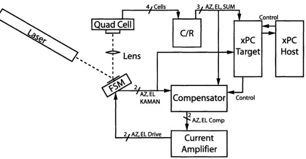
2-1 Diagram of the experimental hardware configuration with signal paths. 30
2-2 Picture of the Thorlabs fiber-coupled laser source, model S1FC675. . 31
2-3 Picture of the collimator used with the fiber-coupled laser source in
mount, courtesy of Paula Ward. . . . . 32
2-4 Picture of the Helium-Neon (HeNe) laser source with 2 axis adjustable
m ount. . . . . 34
2-5 Picture of the focusing lens with 5 axis adjustable mount. . . . . 35 2-6 Generalized schematic of SPOT-4DMI quad cell showing photodiode
elements and output signals. . . . . 38
2-7 Picture of the SPOT-4DMI quad cell, mounted in flight box. . . . . . 39
2-8 Picture of the SPOT-4DMI quad cell, mounted on plastic housing for
use with the UDT Model 431 X-Y Position Indicator. . . . . 40
2-9 Orientation of SPOT-4DMI quad cell in flight box of Figure 2-7. . . . 40 2-10 Diagram of the SPOT-4DMI quad cell's active elements with labeled
ax es. . . . . 4 1
2-11 Picture of the UDT Instruments Model 431 X-Y Position Indicator. . 43
2-12 Picture of the Conversion/Rotation Board as configured for use with
digital compensator, courtesy of Paula Ward. . . . . 44
2-13 Schematic of the conversion circuitry of the C/R Board showing
op-amp math functions and output voltage ranges, originally designed at
Lincoln Laboratory. . . . . 45
2-14 Schematic of rotation circuitry of the C/R Board, including op-amp
m ath functions. . . . . 47
2-15 Picture of the original controller hardware box mounted in rack,
hous-ing the analog compensator, current amplifiers and power supplies. 48
2-16 Generalized feedback control block diagram for control of the FSM. 49
2-17 Schematic of the KAMAN rotation circuitry and summing amplifier
used in feedback control, designed at Lincoln Laboratory. . . . . 50
2-18 Schematic of the original analog compensator used for both KAMAN and quad cell feedback control, designed at Lincoln Laboratory. . . . 51 2-19 Schematic of the high bandwidth current amplifier designed at Lincoln
Laboratory (1/2). . . . . 52
2-20 Schematic of the high bandwidth current amplifier designed at Lincoln
Laboratory (2/2). . . . . 53
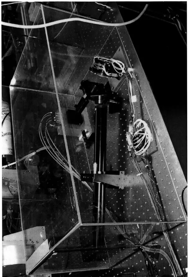
2-21 Picture of the experimental hardware configuration. . . . . 55
2-22 Picture of the experimental hardware setup with Plexiglas shroud. . . 56
2-23 Schematic of the hardware configuration using the original analog
com-pensator with xPC. . . . . 57
2-24 Schematic of the hardware configuration using the digital compensator
w ith xP C . . . .. . . . . . 57
2-25 Diagram of the Simulink model illustrating the A/D, D/A and Digital
I/O capabilities of the General Standards PMC-ADADIO card with
common connection methodology. . . . . 59
2-26 Picture of the GUI used to control the digital compensator running on
the xPC Target PC. . . . . 61
3-1 Picture of the Fast Steering Mirror mounted on an optical table. . . . 66 3-2 Exploded component diagram of the FSM (shown with a smaller
mir-ror), courtesy of James Roberge. . . . . 67
3-3 FSM Azimuth open loop frequency response, KAMAN Voltage Out
/
Driver Voltage In, 10 -20,000 Hz. Data taken with a resolution of 1600
points
/
kHz between 10 Hz and 12 kHz, and 1600 points between 12and 20 kH z. . . . . 70
3-4 Simple model of one axis of FSM. mi represents the part of the FSM
that is directly monitored by the KAMAN sensors, and m2 represents
the decoupling mass. . . . . 71
3-5 Normalized Bode diagram of first "doublet" of the FSM Azimuth axis.
Bode diagram is Position
/
Input Force. . . . . 723-6 FSM Azimuth open loop KAMAN frequency response with parametric
m odel, 10 - 3,000 Hz. . . . . 75
3-7 FSM Elevation open loop frequency response, KAMAN Voltage Out
/
Driver Voltage In, 10 - 20,000 Hz. Data taken with a resolution of 1600
points
/
kHz between 10 Hz and 12 kHz, and 1600 points between 12and 20 kH z. . . . . 76
3-8 FSM Elevation open loop KAMAN frequency response with parametric
m odel, 10 - 3,000 Hz. . . . . 77
3-9 FSM Azimuth and Elevation open loop frequency response overlay,
KAMAN Voltage Out
/
Driver Voltage In, 10 - 20,000 Hz. . . . . 783-10 FSM Azimuth open loop frequency response, quad cell Voltage Out
/
Driver Voltage In, 10 - 20,000 Hz. Data taken with a resolution of 1600
points
/
kHz between 10 Hz and 12 kHz, and 1600 points between 12and 20 kH z. . . . . 80
3-11 Normalized comparison of the FSM Azimuth KAMAN open loop
fre-quency response with the quad cell open loop frefre-quency response, 10
-20,000 H z. . . . . 81
3-12 Normalized comparison of the FSM Azimuth KAMAN open loop
fre-quency response with the quad cell open loop frefre-quency response, 1.5
-3kHz. ... ... 82
3-13 FSM Azimuth open loop quad cell frequency response with parametric model, 10 - 20,000 Hz. . . . . 84
3-14 FSM Elevation open loop frequency response, quad cell Voltage Out
/
Driver Voltage In, 10 -20,000 Hz. Data taken with a resolution of 1600 points/
kHz between 10 Hz and 12 kHz, and 1600 points between 12 and 20 kHz... ... 853-15 FSM Elevation open loop quad cell frequency response with parametric model, 10 - 20,000 Hz. . . . . 86
3-16 Normalized comparison of the FSM Elevation KAMAN open loop fre-quency response with quad cell open loop frefre-quency response, 10 -20,000 H z. . . . . 87
3-17 Normalized comparison of the FSM Elevation KAMAN open loop fre-quency response with quad cell open loop frefre-quency response, 1.2 - 3 kHz ... ... 88
3-18 FSM Azimuth and Elevation Open Loop Frequency Response Overlay, KAMAN Voltage Out
/
Driver Voltage In, 10 - 20,000 Hz . . . . 894-1 Example of a Stateflow diagram . . . . 93
4-2 Stateflow diagram of the square spiral algorithm (1/2). . . . . 96
4-3 Stateflow diagram of the square spiral algorithm (2/2). . . . . 97
4-4 X-Y plot of the steering path of the square spiral algorithm with pitch = 2 and count-max = 3. . . . 102
4-5 Simulink model of the top level xPC implementation for all spiral al-gorithms. .. ... 103
4-6 X-Y plot of the steering path using the CLV spiral algorithm, ... 104
4-7 MATLAB graphical user interface used to control square spiral algorithm. 106 4-8 X-Y plot of steering path showing the effect of changing the 'Spiral Size' value in the square spiral algorithm. . . . 107
4-9 X-Y plot of steering path showing the effect of changing the 'Spiral Resolution' value in the square spiral algorithm. . . . 108
4-10 Stateflow diagram of the constant angular velocity (CAV) spiral algo-rithm . . . 110
4-11 X-Y plot of the steering path of the CAV spiral algorithm with pitch = 5, maxxradius = 10 and freq = 250. . . . 115
4-12 Second level Simulink model of the CAV spiral algorithm . . . 116
4-13 MATLAB graphical user interface used to control the CAV spiral al-gorithm . . . 117
4-14 X-Y plot of the steering path showing the effect of changing the 'Spiral Size' value in the CAV spiral algorithm . . . 119
4-15 X-Y plot of the steering path showing the effect of changing the 'Spiral Frequency' value in the CAV spiral algorithm. . . . 120
4-16 X-Y plot of the steering path showing the effect of changing the 'Spiral
Resolution' value in the CAV spiral algorithm. . . . . 121
4-17 Stateflow diagram of the constant linear velocity (CLV) spiral algorithm. 123 4-18 Diagram showing step progression of CLV spiral algorithm from point
P to pointQ. . . .. . . . .. .. ... .... . ... . . . 126
4-19 X-Y plot of the steering path using the CLV spiral algorithm, showing
the transition from CAV to CLV. . . . . 127
4-20 X-Y plot of the steering path using the CLV spiral algorithm compared
with a MATLAB generated CAV spiral. . . . . 128
4-21 Second level Simulink model of the CLV spiral algorithm. . . . . 130
4-22 MATLAB graphical user interface used to control the CLV spiral
al-gorithm . . . . 131
4-23 X-Y plot of the steering path showing the effect of changing the 'Spiral
Size' value in the CLV spiral algorithm. . . . . 132
4-24 X-Y plot of the steering path showing the effect of changing the 'Spiral
Arc Length' value in the CLV spiral algorithm . . . . 133
4-25 X-Y plot of the steering path showing the effect of changing the 'Spiral
Resolution' value in the CLV spiral algorithm. . . . . 134
4-26 Diagram showing grid points visited during CLV spiral algorithm with
effective coverage of each point. . . . . 135
4-27 Stateflow diagram showing acquisition algorithm used with all spiral
algorithm s. . . . . 136
4-28 Experimental plots showing the FSM steering path and quad cell
po-sition over a 10 V range using the square spiral algorithm. . . . . 138
4-29 Experimental plots showing the distance from the origin of the quad cell and quad cell Optical Sum over a 10 V range using the square
spiral algorithm . . . . 139
4-30 Experimental plots showing the FSM steering path and observed quad
cell position in the linear range using the square spiral algorithm. . . 142
4-31 Experimental plots showing the distance from the origin of the quad cell and quad cell Optical Sum in the linear range using the square
spiral algorithm . . . . 143
4-32 Experimental plots showing the FSM steering path and observed quad
cell position during acquisition using the square spiral algorithm. . . . 145
4-33 Experimental plots showing the distance from the origin of the quad cell and quad cell Optical Sum during acquisition using the square
spiral algorithm . . . . 146
5-1 Simulink model used with analog compensator. . . . . 151
5-2 Block diagram showing rate feedback applied to an underdamped 2 d
order system . . . . 153
5-3 Comparison of the modeled open loop frequency responses of the FSM
Azimuth axis using the quad cell, with and without rate feedback. . . 154
5-4 Block diagram of the feedback control system using the analog compen-sator with rate feedback, with the FSM represented as an underdamped
2"d order system . . . . 155
5-5 Modeled frequency response of the original analog compensator, VlK/Vl t,
from 10 Hz to 100 kHz. . . . 156
5-6 Comparison between the experimental and modeled negative loop
trans-missions of the FSM in quad cell feedback mode using the original
analog compensator with
f,
r 1 kHz. . . . 1585-7 Negative of the loop transmission of FSM Elevation axis in quad cell
feedback mode using the original analog compensator with
f,
a 1 kHz,1.9 kHz To 5 kHz. . . . 159 5-8 Simulated and experimental Nyquist plots of the negative loop
trans-mission of the FSM Elevation axis in quad cell feedback mode using
the original analog compensator with
f,
P 1 kHz. The region near the-1 point shown in detail in Figure 5-9 . . . 160 5-9 Simulated and experimental Nyquist plots of the negative loop
trans-mission of the FSM Elevation axis in quad cell feedback mode using
the original analog compensator with
f,
~ 1 kHz, zoomed in to showthe -1 point. . . . . 161
5-10 Closed loop frequency response of the FSM Elevation axis in quad cell
feedback mode using the original analog compensator with
f,
O 1 kHz,10 Hz To 5 kHz. . . . . 162 5-11 Block diagram of the feedback control system implemented with the
digital compensators, including rate feedback. . . . 164
5-12 Simulink model of the digital compensator. . . . . 165 5-13 Simulink model of the digital compensator with the quad cell rotation
stage . . . . 168
5-14 Simulink model of the digital compensator with quad cell rotation stage
and integrated rate feedback. . . . . 169
5-15 Modeled FSM quad cell azimuth axis with incorporated digital phase
delay shown with original open loop model . . . . 170
5-16 comparison of the FSM quad cell Azimuth axis modeled open loop frequency responses with and without rate feedback near 1 kHz. . . . 171 5-17 Modeled frequency response of Gc (s) with K = .0535, 1 Hz to 100 kHz. 173 5-18 Modeled FSM quad cell Azimuth axis negative loop transmission using
Gc1(s), 5 Hz to 3 kHz. . . . . 174
5-19 Modeled FSM quad cell azimuth axis negative loop transmission using
Gi(s) near crossover. . . . . 175
5-20 Modeled FSM quad cell Azimuth axis Nyquist diagram using G,1(s). 177
5-21 Modeled FSM quad cell Azimuth axis Nyquist diagram using Gc1(s)
near the -1 point. . . . . 178
5-22 Modeled FSM quad cell Azimuth axis closed loop frequency response
using G c1(s) . . . . 179
5-23 Modeled FSM quad cell Azimuth axis step response using Gcj (s). . . 180
5-24 Modeled frequency response of the digital compensator G,2(s). .. .. 182
5-25 Modeled FSM quad cell Azimuth axis negative loop transmission using
Gc2(s) with K = .0435... 183
5-26 Modeled FSM quad cell Azimuth axis negative loop transmission near
crossover using Gc2(s) with K = .0435. . . . . 184
5-27 Modeled FSM quad cell Azimuth axis Nyquist diagram using Gc2(s)
with K = .0435. . . . . 186
5-28 Modeled FSM quad cell Azimuth Axis Nyquist diagram near the -1
point using Gc2(s) with K = .0435. . . . . 187
5-29 Modeled FSM quad cell Azimuth axis closed loop frequency response
using Gc2(s) with K = .0435. . . . . 188
5-30 Modeled FSM quad cell Azimuth axis step response using Gc2(s) with
K = .0435. . . . . 189
5-31 Modeled frequency response of the digital compensator Gc3(S). . . . . 191 5-32 Modeled FSM quad cell Azimuth axis negative loop transmission using
Gc3(s) with K = .043. . . . . 192 5-33 Modeled FSM quad cell Azimuth axis negative loop transmission near
crossover using Ge3(s) with K = .043. . . . . 193
5-34 Modeled FSM quad cell Azimuth axis Nyquist diagram using Gc3(s)
with K = .043. . . . . 194
5-35 Modeled FSM quad cell Azimuth axis Nyquist diagram near the -1
point using Ge3(s) with K = .043. . . . . 195
5-36 Modeled FSM quad cell Azimuth axis closed loop response using Gc3(s)
with K = .043 . . . " . .. 196
5-37 Modeled FSM quad cell Azimuth axis step response using Gc3(s) with
K = .043. . . . . 197
5-38 Experimental FSM quad cell Azimuth axis negative loop transmission
using Gc2(s) with K = .0435, 5 Hz - 3 kHz. . . . . 199
5-39 Experimental FSM quad cell Azimuth axis negative loop transmission
near crossover using Gc2(s) with K = .0435, 2.25 - 3 kHz. . . . . 200
5-40 Experimental FSM quad cell Azimuth axis Nyquist diagram using
Gc2(s) with K = .0435. . . . . 201 5-41 Experimental FSM quad cell Azimuth axis Nyquist diagram near the
-1 point using Gc2(s) with K = .0435. . . . . 202 5-42 Experimental FSM quad cell Azimuth axis closed loop frequency
re-sponse using G,2(s) with K = .0435. . . . . 203
5-43 Experimental FSM quad cell Azimuth axis normalized step response
using Gc2(s) with K = .0435. . . . . 204
5-44 Experimental FSM quad cell Azimuth axis negative loop transmission
using Gc3(s) with K = .0210, 5 Hz - 3 kHz. . . . . 206
5-45 Experimental FSM quad cell Azimuth axis Nyquist diagram near the
-1 point using G,3(s) with K = .0210. . . . . 207
5-46 Experimental FSM quad cell Azimuth axis closed loop frequency
re-sponse using Gc3(s) with K = .0210. . . . . 208 5-47 Experimental FSM quad cell Azimuth axis normalized step response
using Ge3(s) with K = .0210. . . . . 209
5-48 Experimental FSM quad cell Azimuth axis negative loop transmission
using Ge3(s) with K = .0336, 5 Hz - 3 kHz. . . . . 211
5-49 Experimental FSM quad cell Azimuth axis Nyquist diagram near the
-1 point using G,3(s) with K = .0336. . . . . 212 5-50 Experimental FSM quad cell Azimuth axis closed loop frequency
re-sponse using G,3(s) with K = .0336. . . . . 213
5-51 Experimental FSM quad cell Azimuth axis normalized step response
using Gc3(s) with K = .0336. . . . . 214
A-1 Simple model of one axis of FSM. mi represents the part of the FSM
that is directly monitored by the KAMAN sensors, and m2 represents
the decoupling mass. . . . 223
List of Tables
4.1 Table of Stateflow input variables used in the square spiral algorithm. 98
4.2 Table of Stateflow output variables used in the square spiral algorithm. 99
4.3 Table of Stateflow local variables used in the square spiral algorithm. 100
4.4 Table of Stateflow input variables used in the CAV spiral algorithm. . 111
4.5 Table of Stateflow output variables used in the CAV spiral algorithm. 112
4.6 Table of Stateflow local variables used in the CAV spiral algorithm. . 113
4.7 Table of Stateflow input variables used in the CLV spiral algorithm. . 124
4.8 Table of Stateflow output variables used in the CLV spiral algorithm. 125
4.9 Table of Stateflow local variables used in the CLV spiral algorithm. . 125
5.1 Experimental performance specifications of the FSM quad cell
Eleva-tion axis using the original analog compensator. . . . . 157
5.2 Modeled performance specifications of the FSM quad cell Azimuth axis
using Ge (s), both with and without rate feedback. . . . 181
5.3 Modeled performance specifications of the FSM quad cell Azimuth axis
using G,2(s), both with and without rate feedback. . . . 190
5.4 Modeled performance specifications of the FSM quad cell Azimuth axis
using Gc3(s), both with and without rate feedback. . . . 198
5.5 Experimental performance specifications of the FSM quad cell Azimuth
axis using Gc2(s) without rate feedback and K = 0.0435. . . . . 205
5.6 Experimental performance specifications of the FSM quad cell Azimuth
axis using Gc3(s) with rate feedback and K = .0210. . . . 210
5.7 Experimental performance specifications of the FSM quad cell Azimuth
axis using G,3(s) with rate feedback and K = .0336. . . . . 215
Chapter 1
Introduction
1.1
MarsComm Summary
In an effort to better understand the solar system, NASA and the United States gov-ernment have decided to send several unmanned vehicles to Mars in the next decade. Current communication between the Earth and the orbiters takes place via high frequency radio transmission. This technology is several decades old, and has the ad-vantage of being space proven and relatively easy to implement. However, even with directional antennas, much of the power used in radio communication is wasted as the waves radiate in many directions, with only a small percentage of the transmitted power reaching the receiver. NASA has decided to implement a laser-based commu-nication system designed to achieve higher bandwidth data transfers with much less wasted power. The Mars Laser Communication Demonstration (MarsComm) pro-gram is the implementation of this laser-based communication onboard an orbiter.
Unlike radio waves, lasers can be highly focused at the transmission point. This is due to the difference in relative wavelengths. Deep space radio transmissions operate near the GHz range, giving them a wavelengths between 10 m and 10 cm, where lasers operate in the infrared or visible spectrums with wavelengths between 100 Am and 400 nm. The shorter wavelength lasers can be better focused, giving them a
tighter angular dispersion pattern and greater power densities (W/m 2) for the same
transmission power and distance. This allows for much less power to be used in
communication, but introduces a problem of pointing. The less tightly confined radio waves do not have to be pointed at the receiver more accurately than a few degrees, but the tighter confined laser must be pointed with much greater accuracy. The lasers
used in MarsComm disperse to a diameter of approximately 1/6th the Earth's radius
over the trip from Mars to Earth. To hit the communication ground station on Earth, the laser must be pointed with no more than 400 nanoradians RMS error between 1 Hz and 1 kHz.
This pointing accuracy requirement one of the key challenges for making MarsComm a viable technology. Several pieces are required to make the system work. A system diagram is shown in Figure 1-1. This schematic shows the signal path of a laser beam emitted from the Earth. The main parts of the system include a Magnetohydrody-namic Inertial Reference Unit (MIRU), a Fast Steering Mirror (FSM), a quad cell optical detector and a focal plane array (FPA).
1.1.1
The MIRU
The MIRU provides an inertial reference unit for the spacecraft. This is accomplished
by using Magnetohydrodynamic (MHD) sensors. The MHD sensors used, Part
#
ARS-12B, are produced by Applied Technology Associates (ATA)[1]. These sensors provide angular rate information from 2 Hz to about 1 kHz. Because the MHDs are rate sensors, the system is AC coupled. Angular position information below 2 Hz is provided by the FPA, an IR sensitive imaging unit. This low frequency information is blended with the MHD sensors to provide feedback from DC to about 1 kHz. Using this feedback information, the MIRU is able to provide an inertially stable reference frame aboard the spacecraft with the crossover frequency of about 300 Hz.
1.1.2
The Fast Steering Mirror
The MIRU provides an inertial reference on board the spacecraft, but it does not correct for the error between the spacecraft motion ("jitter") and its inertially stable motion. This correction is accomplished with the Fast Steering Mirror. The MIRU
Beacon* Earth 2 2-300 Hz active A > 300 Hz passive MIRU 77747777 A
BLENDING TRACK LOOP DC - 2 HZ I' I I
K'
FSM --Quad Cell I I I...
...
FPAFigure 1-1: Simplified MarsComm spacecraft signal path schematic, courtesy of Jamie Burnside.
25
... 1400 0, ... ... 4 ... I
-beams a laser along the same optical path as the Earth bound laser -beams. This beam bounces off of the FSM and hits a quad cell detector. At the zero state with no relative motion between the Earth and the spacecraft, the MIRU will not be active, the FSM will not be active and the laser will hit the center of the quad cell. As the spacecraft jitter introduces angular error in the pointing of the beam, the MIRU stays inertially stable, and the FSM uses this inertially stable reference beam to zero out the quad cell and restore the optical path as if the spacecraft had not moved. The current control system for the FSM has a crossover frequency of 1 kHz and a closed loop bandwidth of 2 kHz. If the bandwidth of the FSM could be pushed up, it would decrease the RMS angular error of the system and make the other system component noise requirements lower, leading to lower costs. Before redesigning the
FSM hardware, it is prudent to investigate if the performance can be improved via a
better controller design that can be easily integrated into the system.
1.2
Thesis Overview
The goal of this thesis is to find the best controller for the FSM, given its hardware characteristics.
Chapter 2 describes the rest of the hardware used in the experiments. Several testing configurations are presented along with an overview of the integration of the
hardware with the software control system.
Chapter 3 focuses on the actual FSM hardware. Prior research and design of the
FSM is presented, including individual component descriptions along with schematics.
Detailed open loop frequency analysis of each axis is presented along with parametric models for computer simulations.
Chapter 4 details the design of a spiral acquisition algorithm used to initially point the FSM onto the active region of the quad cell, used to switch between KAMAN and quad cell control.
Chapter 5 details the control theory behind the current analog compensator in use. The design of an original compensator to push the FSM to its hardware limits
is presented along with experimental results.
Chapter 6 details the conclusions of the controller design and recommendations for future work.
Chapter 2
Hardware Overview
This chapter describes the hardware used during the experimentation process. Sec-tion 2.1 describes each piece of hardware used during experimentaSec-tion in detail, in-cluding electronic schematics where appropriate. Section 2.2 describes the physical layout of the hardware during experimentation, including wiring diagrams and pic-tures of the test setups. Finally, Section 2.3 describes how xPC was used to control the experiments, including the design and implementation of graphical user interfaces
(GUIs) and the basic components of the Simulink models used.
2.1
Hardware Components
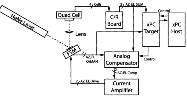
This section details all of the hardware used in the experiments controlling the FSM. Figure 2-1 shows the general layout of the experiment with all the relevant hardware. The ordering of this section follows the beam path of the laser in the experiment.
2.1.1
Laser Sources
The laser sources used in the experiment simulate the laser beam produced by the MIRU. Two separate laser sources were used in these experiments, as described below.
44 Cells 3 AZ, EL, SUM
j J C/R -+r
erxPC xPC
Lens .Ta rg et Host
AZ, EL
KAMAN
Compensator
Control 2AZ, EL Comp 24 AZEL DriveU
~ Current
Amplifier
Figure 2-1: Diagram of the experimental hardware configuration with signal paths.
Fiber-Coupled Source
The Thorlabs S1FC675 fiber-coupled laser source was used in early experimentation. The MIRU is designed to use a fiber-coupled source, and thus using the source is a good approximation to the actual flight hardware. The laser outputs a red gaussian laser beam at 675 nm into a fiber. The output power of the laser source is controllable between 0 and 2.5 mW. Further attenuation of laser power is accomplished with a neutral density optical filter. The power level of the laser must be controlled so as not to saturate the quad cell and position indicator electronics (see Section 2.1.5). The output of the fiber is fed into a collimator, shown in Figure 2-3. The final output at the collimator is a circular gaussian beam with a diameter of approximately 5 mm.
Unfortunately, during experimentation, the fiber-coupled laser source introduced a variety of problems. The laser output cross sectional power (the spot size on the
quad cell and the distribution of power on that spot) varied greatly when the fiber was moved or jostled. This movement was not extreme in the short term; however, the drift was noticeable after several minutes. The spot often drifted off the active region of the quad cell within 30 minutes. The cause of this drifting has not been
Figure 2-2: Picture of the Thorlabs fiber-coupled laser source, model S1FC675.
Figure 2-3: Picture of the collimator used with the fiber-coupled laser source in mount, courtesy of Paula Ward.
identified; however, due to time constraints with the project, a different laser source was implemented with much better results.
Helium-Neon (HeNe) Laser Source
The Helium-Neon (HeNe) Laser used during the experiments is shown in Figure 2-4. The laser is approximately 40 cm long with a tube diameter of approximately 7 cm. The laser is held in a mount at its midpoint and attached to the table. The mount allows the laser to be moved in two angular axes. This speeds up alignments procedures, but is not necessary in the final configuration of the hardware. With the mount in place, the natural frequency of the laser system is approximately 66 Hz (which was discovered after trying to debug 60 Hz noise). This is due to the fact that the mounting of the laser creates a large cantilever system, much like a see-saw. Placing the laser on blocks would eliminate this natural frequency, but would not allow adjustment of the laser orientation. The laser outputs a green (535 nm) gaussian circular spot approximately 1 mm in diameter at 20 cm from the laser aperture. The maximum power output of the laser is 5 mW, but has been measured to be no more than 3 mW nominal power. The output of the laser is attenuated by a neutral density optical filter directly after the laser aperture. The output power level is set by the quad cell limits (see Section 2.1.5).
2.1.2
The FSM
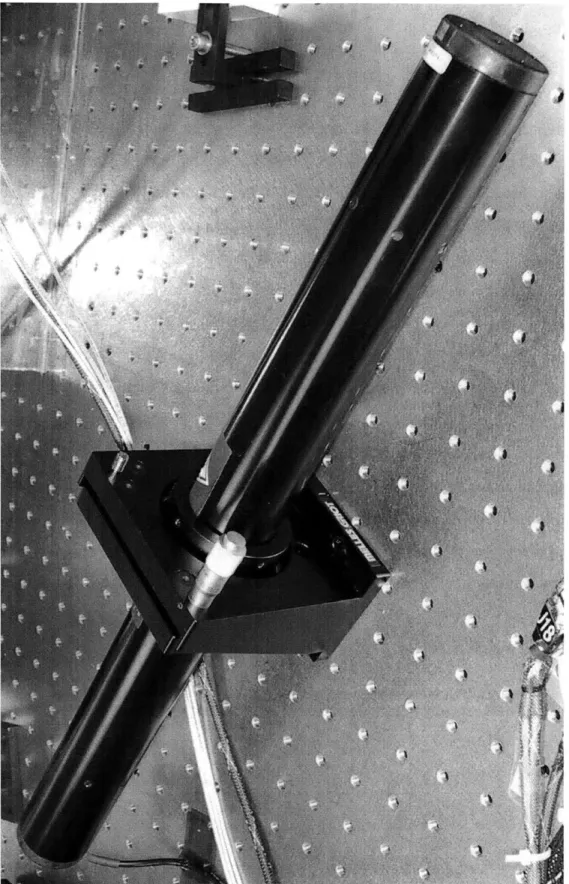
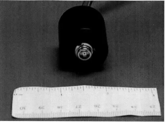
The laser source beam exits and reflects off of the Fast Steering Mirror. The mirror is used to control where the spot hits the quad cell. The FSM is discussed in detail in Chapter 3.
2.1.3
Focusing Lens
A lens is necessary to focus the laser beam onto the quad cell. The lens used in the
experiments is shown in Figure 2-5.
The lens used is a standard convex lens with a focal length of approximately 15
Figure 2-4: Picture of the Helium-Neon (HeNe) laser source with 2 axis adjustable mount.
Figure 2-5: Picture of the focusing lens with 5 axis adjustable mount.
cm. This lens focuses the laser beam onto the active area of the quad cell (which
is approximately 1 mm2). The mount for the lens allows manipulation of the lens
in 5 different axes. This mount was necessary in the testing phase to keep the FSM near the center of its operating region without having to realign the optical hardware. However, skewing can occur if the lens must be placed at gross angles relative to the quad cell. This was not a problem during experimentation because the HeNe laser was adjusted first to eliminate gross angular errors and the lens mount was only used for fine adjustments.
2.1.4
xPC Control
Control of the hardware in the experiments is handled by a part of MATLAB called xPC. xPC is actually run on two separate computers during an experiment.
xPC Target
One computer, known as the xPC Target, runs a very basic kernel of xPC, bypassing all the software complexities of Windows and other operating systems. This bare ker-nel allows the computer to run programs at very high sampling rate. The programs that run on the Target are created in Simulink. The Simulink models run on the Tar-get PC, simulating the desired system, such as a basic controller or a data acquisition device. Input and outputs are passed through between 1 and 4 General Standards PMC-ADADIO cards. Each card has 8 Analog Inputs, 4 Analog Outputs and 8 Dig-ital I/O channels. Standard operating frequency of the xPC Target Simulink model
is 10 kHz, but simple models can be run as high as 50 kHz.
xPC Host
While the xPC Target is running, parameters in the Simulink model can be changed in real time to alter the functionality of the model. This control is accomplished via an ethernet link between the xPC Target PC and an additional PC, called the xPC Host. MATLAB is running on the xPC Host machine, and parameters can be
changed on the Target machine via the MATLAB command line. The model running on the Target PC can also be started, stopped or reloaded via the xPC Host PC. For ease of use, graphical user interfaces (GUIs) can be written in MATLAB and run on the Host PC to control the Target PC.
2.1.5
The Quad Cell
The quad cell is the heart of the optical tracking loop. The quad cells used in these experiments are all SPOT-4DMI quad cells made by UDT Sensors, Inc. The quad cell itself is simply 4 very small, very sensitive photodiodes arranged in a small grid.
Figure 2-6 shows the schematic of the quad cell.
Each active element of the quad cell (A, B, C or D) has an active area of 0.25
mm2, giving a combined total active area of 1 mm2. Of this active area, only the
middle 25% is linear. Non-linearities occur past the inner 25%, becoming extreme past about 75%. The gaps between the elements are 13 Mm wide. Each of these 4 elements outputs a voltage proportional to the amount of light hitting it. There are two packages used in the experiments. These two packages are shown in Figures 2-7 and 2-8. Each package contains the same SPOT-4DMI quad cell, but outputs to a different conversion board. In order to calculate the position of the laser beam, the 4 element voltages outputted from either package must be converted into Azimuth and Elevation signals. This task is accomplished via conversion hardware.
The quad cell in Figure 2-7 is mounted at a 45' angle in the flight box (due to packaging constraints). Figure 2-9 shows the orientation of the quad cell. Because of this packaging, the converted Azimuth and Elevation signals must be rotated by 450.
2.1.6
Conversion/Rotation Hardware
The quad cell packages shown in Figures 2-7 and 2-8 both output 4 element voltages corresponding to the intensity of light on each photodiode. This information must be converted into Azimuth and Elevation position information to be useful to the controller hardware. Each package requires a different method of conversion, and if
Cf Rf A Rf V
A
B
100OpF Cf Rf Cf RfD
C
Cf Rf 4-BFigure 2-6: Generalized schematic of SPOT-4DMI quad cell showing photodiode elements and output signals.
Figure 2-7: Picture of the SPOT-4DMI quad cell, mounted in flight box.
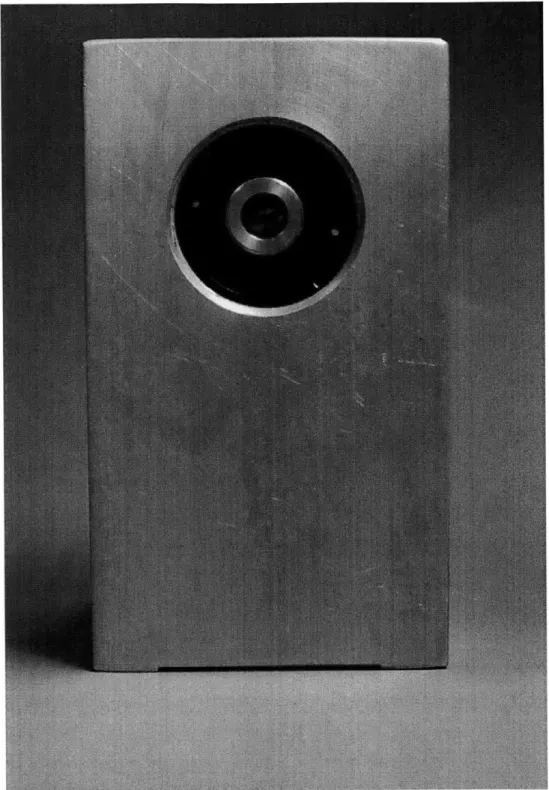
Figure 2-8: Picture of the SPOT-4DMI quad cell, mounted on plastic housing for use with the UDT Model 431 X-Y Position Indicator.
Figure 2-9: Orientation of SPOT-4DMI quad cell in flight box of Figure 2-7.
necessary, rotation.
Conversion Algorithm
The basic math required to obtain Azimuth and Elevation from the quad cell is straightforward. Using the orientation of the quad cell elements as shown in Figure
2-10, the basic Azimuth and Elevation voltages are as follows:
AZ- (C+D)-(A+B) (A + B+C + D) EL(A + D) -(B+C) (A+B+C+D)
A
B
(2.1) (2.2) ELD
AZC
Figure 2-10: Diagram axes.of the SPOT-4DMI quad cell's active elements with labeled
Equations 2.1 and 2.2 are easy to understand. If the laser spot was circular and focused directly at the center of the quad cell, the voltages on each element would be the same and the Azimuth and Elevation voltages would both be zero, as expected. This reasoning would hold no matter what the size of the spot was (as long as it was all contained in the active region of the quad cell). Furthermore, the reasoning still holds if the spot is not circular, but rather a skewed ellipse. This works because
the Azimuth voltage is essentially the left side of the quad cell minus the right, and the Elevation is the top minus the bottom. A centered ellipse would have equal components left and right, as well as top to bottom, and thus would still register zero volts for both Azimuth and Elevation. For this reason, quad cells are said to be "centroid" friendly, as they tend to output the centroid of a spot, no matter its specific shape.
UDT X-Y Position Indicator
Figure 2-11 shows the UDT Instruments Model 431 X-Y Position Indicator used with the quad cell package shown in Figure 2-8. This position indicator is a single box solution for quad cell signal conversion. The quad cell is plugged into the position in-dicator, and the hardware outputs the Azimuth, Elevation, and Optical Sum voltages. The Optical Sum voltage is the sum of the voltages on each of the 4 photodiodes, and is useful in determining if the beam is on the active region of the quad cell. Azimuth and Elevation are outputted analog voltages, +1 Vpk. The Optical Sum voltage is always positive, ranging up to 10 Vpk.
The 431 Position Indicator has a front end amplifier designed to allow adjustment for different incident beam strengths. This amplifier allows the use of different lasers or different laser powers without adjusting the neutral density filtering. This amplifier should be set so that the Optical Sum voltage is between 300 and 1000 on the Sum display.
Rotation is not possible with the Model 431. The quad cell package must be aligned to the FSM in experiment. This is more difficult than it would seem, and the mounting hardware for this quad cell Package was very cumbersome. The original mounting had 5 degrees of freedom, leading to the addition of several low frequency modes that interfered with data collection. This setup was used only very early on in testing, giving way to the quad cell flight package shown in Figure 2-7. However, the flight package is not compatible with the Model 431 and a Conversion/Rotation
Board had to be built to interface with the quad cell.
Figure 2-11: Picture of the UDT Instruments Model 431 X-Y Position Indicator.
C/R Board
As was stated before, there is no commercial solution to convert the 4 element outputs of the quad cell flight package shown in Figure 2-7. However, Lincoln Laboratory has designed hardware for this exact purpose. The hardware is flight approved, but was not available for use during this project. Instead, the schematics were made available, and after small modifications, an analog Conversion/Rotation board was built. This board is shown in Figure 2-12.
The bottom half of the C/R Board handles the conversion from 4 element voltages to non-rotated Azimuth and Elevation voltages. The schematic for the conversion is shown in Figure 2-13. The inputs to this part of the board are the 4 element voltages A, B, C, and D. The outputs are the two non-rotated Azimuth and Elevation voltages, AZNR and ELNR respectively. The Optical Sum voltage, QSUM, is outputted at the top of the board as well.
The top half of the C/R Board handles the rotation of the Azimuth and Elevation signals from the conversion half of the board. As stated before, this rotation is
necessary because the SPOT-4DMI quad cell is mounted at a 450 angle in the flight
box. A simple rotation matrix is used to rotate the two signals. To rotate a set of
Figure 2-12: Picture of the Conversion/Rotation Board as configured for use with digital compensator, courtesy of Paula Ward.
O 'o C+ C -4 1- . 0 -15V 47 +15_B 1uF A 10k B 10k 10k C 10k - v. _Q AZ D 10k + 0k Q_AZ = (C + D) - (A + B) -10 - 10 [V] -15V 47 -15_B luF
Power Supply Bypass
1 for each Component
B 10k C 10k 10k A 1 k QQE D 10k 10k QEL =(A + D) -- (B + C) -10 - 10 [V] A 10k 10k B 10k 15k C 10k Q SUM D 10k + 10k Q_SUM = (A + B + C + D) / 2 0 - 10 [V] Q SUM AD534LD X2 D AZ NR - U2 Z2 -- Yi ER, - Q AZ Y2 V--10k
AZNR =10 * QAZ /QSUM
-10 - 10 [V] Q SUM AD534LD - xi V+. --X2 DD- - EL NR -U0 W. ~ --- U1 Zl--U2 Z2, - -- - ---Y1 ER - Q EL Y2 V-1-7 10 kl -_ EL NR = 10 *Q EL / Q SUM - -10 -10 [V]
orthogonal axes clockwise by an angle 0, the signal vector is multiplied as follows:
cos 0 - sin 0 AZ AZrt (2.3)
Lsin 0 cos 0 L EL ELrot
When rotating 450 clockwise, equation 2.3 simplifies to
AZt = /-
(AZ
- EL) (2.4)2
ELrot = . (AZ + EL) (2.5)
2
Ignoring the x/2/2 factor for the moment, rotating the axes 45*is as simple as either adding or differencing the Azimuth and Elevation signals. In fact, to rotate
any multiple of 450 involves just a combination of adding and differencing the Azimuth
and Elevation signals. This is precisely what the upper half of the C/R accomplishes, using two inverting summers. The schematic for the rotation hardware is shown in Figure 2-14. The input and output voltage ranges for the rotation hardware is +10
V. The Vf/2 gain factor is applied by adding a resistive voltage divider network to
the end of the output. In this way, the gain of the quad cell voltage can be lowered as necessary. The V"/2 gain factor cannot be implemented directly into the op-amp math functions, as it would introduce a gain of less than 1, causing the op-op-amp circuitry to be unstable (the op-amps used are unity-gain stable).
The switches in Figure 2-14 are actually jumper blocks that select either the positive or negative version of a signal. These jumpers allow the quick changing of the rotation behavior as necessary.
2.1.7
Analog Compensator
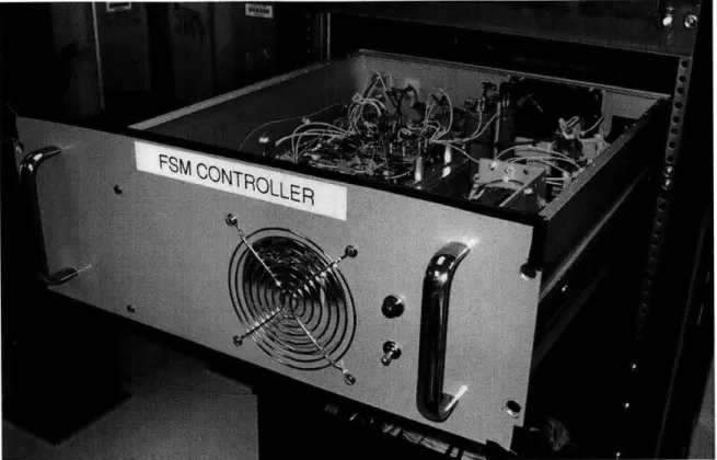
Before this work began, the FSM was controlled by an analog compensator originally designed by MIT professor James K. Roberge at Lincoln Laboratory. Figure 2-15 shows a picture of the entire Controller hardware rack. The Controller hardware rack houses the Analog Compensator, the current amplifiers and the analog and digital
10k AZNR 10kAZ NRN AZNR N -AZNR 10k ELNR1kEL NR N ELNR N = -EL NR 15V 47 +15 B luF -15V 47 -15 B luF AZNR V 1 10k 1+V A ZNR N-1k AZ ROT ELNR V_2 10k EL NRN N-AZ ROT =- (V_1 + V_2) AZNR AZNRN -(V1+k ELROT ELNR 4 v_2 10k EL NR N EL ROT =-(V-1 + V-2)
Power Supply Bypass
1 for each Component
Figure 2-14: Schematic of rotation circuitry of the C/R Board, including op-amp
math functions.
power supplies.
Figure 2-15: Picture of the original controller hardware box mounted in rack, housing the analog compensator, current amplifiers and power supplies.
The compensator was designed to control the FSM in either KAMAN or quad cell feedback mode with the flip of a digital switch. Both sensors use the same generic feedback control. The block diagram for the control of the FSM is shown in Figure
2-16.
Included before the compensator are electronics used to rotate the KAMAN sen-sors 450 for use in the feedback path. The rotation is accomplished much in the same way as the rotation of the quad cell Azimuth and Elevation. The schematic for these electronics is shown in Figure 2-17. This schematic also contains the KAMAN feed-back summing junctions. The overall circuit shown in Figure 2-17 takes in both the
KAMAN sensor voltages and the commanded voltages, and outputs the difference
between the two, just as shown in Figure 2-16. The quad cell Azimuth and Elevation channels are also added together with the appropriate command voltages in the same
Command [V] Error [V] Compensator Amplifier s FSM
I]Sensor
-Figure 2-16: Generalized feedback control block diagram for control of the FSM.
manner. However, no rotation circuitry for the quad cell is present.
The schematic for the compensator is shown in Figure 2-18. The compensator takes in output of the KAMAN or quad cell summing junctions (also known as the Error term), and outputs a voltage intended for a current amplifier. This compensator is used for both feedback sensors, but a digital switch allows only one sensor to be active at a time. Thus, the first op-amps in Figure 2-18 only see either the KAMAN voltage or the quad cell voltage, but never both. For a more detailed review of this original compensator with experimental results, see Section 5.1.
2.1.8 Current Amplifier
The final elements of the control system are the current amplifiers. The current amplifiers take a voltage command from the compensator and drive the voice coil actuators of the FSM as appropriate. The bandwidth of these current amplifiers is sufficiently high as to not introduce any noticeable dynamic behavior in the frequency ranges of interest. The schematic for one of the current amplifiers is broken up between Figures 2-19 and 2-20.
2.2
Testing Configurations
Two main testing configurations were used in benchmarking the performance of the
FSM. The first configuration is the baseline configuration designed to work with the
R59 10k R6120k R39 10k CD aq CD 0CD 0 c~ CD Ki COMMAND R40 10k R58 U6 FSM K2 10k UP4A0 -15 GND R63 R41 20k 10k R57 20k U16B 0P400 4-- 15 GND R56 10k 15 GND C6 100pF