Counting votes right : strategic voters versus strategic parties

Counting Votes Right: Strategic Voters versus Strategic Parties

by

Giovanni Reggiani

M.Sc. Economics and Social Sciences, Bocconi University (2010)

B.A. Economics and Social Sciences, Bocconi University (2008)

Submitted to the Department of Economics

in partial fulfillment of the requirements for the degree of

Master of Science in Economics

at the

MASSACHUSETTS INSTITUTE OF TECHNOLOGY

June 2016

@

2016 Giovanni Reggiani. All rights reserved.

MASSACHUSElTS INSTITUTE

JUN 10

2016

LIBRARIES

ARCHNEB

The author hereby grants to MIT permission to reproduce and distribute publicly paper

and electronic copies of this thesis document in whole or in part.

/71

A-1?

AuthorSignature

redacted

...

Department of Economics

May 15, 2016

/

7$

Signature redacted

Certified by

...

... ...

.

Abhijit Banerjee

Ford Foundation International Professor of Economics

Thesis Supervisor

Accepted by...Signature

redacted

Ricardo J. Caballero

Ford International Professor of Economics

Chairman, Departmental Committee on Graduate Studies

The author hereby grants to MIT permission to reproduce and to

distribute publicly paper and eetoonic copies of this thesis

document

77 Massachusetts Avenue

Cambridge, MA 02139

http://Iibraries.mit.edu/ask

DISCLAIMER NOTICE

Due to the condition of the original material, there are unavoidable

flaws in this reproduction. We have made every effort possible to

provide you with the best copy available.

Thank you.

The images contained in this document are of the

,best

quality available.

Counting Votes Right: Strategic Voters versus Strategic Parties

by

Giovanni Reggiani

Submitted to the Department of Economics on May 15, 2016, in partial fulfillment of the

requirements for the degree of Master of Science in Economics

Abstract

This thesis, joint with F. Mezzanotti, provides a lower bound for the extent of strategic voting. Voters are strategic if they switch their vote from their favorite candidate to one of the main contenders in a tossup election. High levels of strategic voting are a concern for the representativity of democracy and the allocation efficiency of government goods and services. Recent work in economics has estimated that up to 80% of voters are strategic. We use a clean quasi experiment to highlight the shortcomings of previous identification strategies, which fail to fully account for the strategic behavior of parties. In an ideal experiment we would like to observe two identical votes with exogenous variation in the party victory probability. Among world parliamentary democracies 104 have a unique Chamber, 78 have two Chambers with different functions, and only one nation has two Chambers with the same identical functions: Italy. This allows us to observe two identical votes and therefore a valid counterfactual. In addition, the majority premia are calculated at the national level for the Congress ballot and at the regional level for the Senate ballot. This provides exogenous variation in the probability of victory. Because the two Chambers have identical functions, a sincere voter should vote for the same coalition in the two ballots. A strategic voter would instead respond to regions' specific victory probabilities. We combine this intuition with a geographical Regression Discontinuity approach, which allows us to compare voters across multiple Regional boundaries. We find much smaller estimates (5%) that we interpret as a lower bound but argue that it is a credible estimate. We also reconcile our result with the literature larger estimates (35% to 80%) showing how previous estimates could have confounded strategic parties and strategic voters due to the use of a non identical vote as counterfactual.

Thesis Supervisor: Abhijit Banerjee

Contents

Acknowledgements 5

1 Counting Votes Right: Strategic Voters versus Strategic Parties 6

1.1 Introduction ... ... 8

1.2 Background Information ... ... 10

1.2.1 The Parliament ... ... 10

1.2.2 Electoral Law . ... ... .... . .. . 10

1.3 A Simplified Framework ... . 11

1.3.1 A numerical Exam ple: ... 12

1.3.2 A general set up ... .... ... .. .... . .. . 13

1.4 Data and Empirical strategy ... ... 15

1.4.1 D ata . . . . 15

1.4.2 Introduction to the Empirical Strategy ... 16

1.4.3 The Regression Discontinuity test at the National Level ... 18

1.4.4 A case study example: Lombardy vs. Emilia-Romagna . . . . 20

1.4.5 Results and Robustness . . . . 23

1.5 D iscussion . . . . 24

1.6 Strategic parties or strategic voters? . . . . 26

1.7 Conclusions . . . . 31

References 32

Acknowledgements

I am tremendously grateful to my advisor Abhijit Banerjee. Abhijit's deep insights and knowledge have been invaluable in guiding me through every turn of this research. I cannot thank him enough. I am also tremendously indebted for his mentorship, support, and encouragement throughout the whole graduate program.

I would also like to thank Daron Acemoglu and Ben Olken for all their feedback, which has substantially improved my research. Alberto Alesina has been extremely generous with his time outside the MIT Eco-nomics Department. I have the deepest gratitude for my earlier mentors in ecoEco-nomics: Eliana La Ferrara and Pierpaolo Battigalli. Their teaching and investment in me opened the doors to MIT and to the opportunities I have been blessed with.

I have been extremely fortunate to conduct this research with an amazing coauthor and great friend. I am grateful for all I have learned with and from Filippo Mezzanotti. I thank Roberto and Silvia for their love, unconditional support, and constant encouragement. Above all, thanks to my parents Domenico and Franca, to whom I owe everything.

Chapter 1

Counting Votes

Right:

Strategic

Voters

Counting Votes Right: Strategic Voters versus Strategic Parties

by

Giovanni Reggiani

M.Sc. Economics and Social Sciences, Bocconi University (2010)

B.A. Economics and Social Sciences, Bocconi University (2008)

Submitted to the Department of Economics

in partial fulfillment of the requirements for the degree of

Master of Science in Economics

at the

MASSACHUSETTS INSTITUTE OF TECHNOLOGY

June 2016

@ 2016 Giovanni Reggiani. All rights reserved.

The author hereby grants to MIT permission to reproduce and distribute publicly paper

and electronic copies of this thesis document in whole or in part.

A u th or ...

...

Department of Economics

May 15, 2016

A ccep ted by ...

Ricardo J. Caballero

Ford International Professor of Economics

Chairman, Departmental Committee on Graduate Studies

1.1

Introduction

In the political economy literature, strategic voters are defined as citizens that would switch to their preferred contender party from their ideologically favorite one to avoid wasting their vote when a district is pivotal and too close to call. A careful estimation of the extent of strategic voting is the main objective of this paper.

A high fraction of strategic voters would be detrimental both for the representativity of the political system and for the level of competition among parties. Consider the case of a fully strategic population of voters uniformly distributed between a radically left and right parties. The great majority of these voters would prefer a centrist party to be in power but none of them would switch their vote from their preferred extremist party to the centrist because they would anticipate that this would give victory to the opposite wing. In this example we see how strategic voting can prevent external competition against status quo parties, and therefore limit moderating political competition as well as the candidates quality enhancement. It could well be that the majority of the population is exasperated with the extremism of the two main parties but yet, because of their strategic behavior, refuses to vote for a third centrist party that better represents their views (Duverger (1959)).

It's important to note that the representativeness of the elected parties is not a philosophical concern about Democracy, rather an economic one. Governments are responsible for the level, allocation, and quality of public goods, transfers and services for a share of between 30% to 50% of GDP in developed democracies. Therefore if, due to strategic voting, representative democracy is not an effective way to convey the prefer-ences of the citizens, the efficiency of the allocation of government spending is a first order economic concern as both parties that receive votes in equilibrium could make decisions inconsistent with citizens' preferences. Because of these concerns, understanding the extent of strategic voting is a central question to evaluate the functioning of modern democracy. Recent work in economics has estimated the fraction of strategic voters to be 70% (Kawai and Watanabe (2013a)). If a majority of voters are indeed strategic, there is no easy fix with a change of electoral rules, Satterthwaite (1975) showed that for electoral systems to be strategy proof they need to be either dictatorial or non deterministic. In the present work, we apply a new geographical RD methodology (Pinkovskiy (2013)) and a conceptual insight on the importance of comparing two identical votes to derive much smaller estimates (5%) that reassure us on the fact that strategic voting is not a first order concern for democracy and for the economic efficiency of government services.

We argue that previous larger estimates are due to the use of non identical votes which makes controlling for strategic behavior by parties increasingly difficult. Indeed, the main parties also have incentives to behave strategically in a tossup district; via enhanced allocation of resources to the district, selection of more appealing candidates, or shaping policy towards the constituents of such district. As a result even sincere supporters for minority parties may vote for one of the two main contenders not because they are

strategic but because the strategic behavior of parties has accommodated their preferences.

Our identification strategy exploits the uniqueness of the perfect Italian bicameralism and a recent temporary change in the electoral law, which asymmetrically assigned the majority premium between the Congress and the Senate, to observe two identical votes and to have variation in the pivotality and significance of the vote. We consider the difference in the share of votes of the top two Coalitions across the two Chambers in each municipality as the outcome variable. These two Coalitions are the only true contenders for the electoral victory and therefore the only two that could be positively affected by strategic voting. By considering the within Municipality difference in votes across the two Chambers we remove any factor that affects voters actions symmetrically in the two Chambers. We then test whether our outcome variable is affected by the regional changes in electoral strategic incentives. If we consider the municipalities on the border, we can exploit multiple geographical discontinuities with different treatments by using a two-step geographic RD estimator recently developed by Pinkovskiy (2013). In light of this new approach and the two identical votes setup, we find significant but very small estimates, consistent with the important contribution of strategic parties to total misalligned voters.

To understand the role and necessity of each part of our empirical strategy let us think about the ideal test we would like to run. In an ideal randomized controlled trial, we would like to observe how the vote of the same individual changes when we change her beliefs about the probability of being pivotal. We argue that our empirical strategy is as close as possible to this ideal benchmark. The Italian Constitution perfect bicameralism, i.e. the fact that the two Charnbers perform the same functions, allows us to observe two identical votes. The fact that the majority premiums are determined at the Regional level (Senate) and the National level (Congress) allows us to have exogenous variation in the probability of being pivotal. In addition, the difference between the outcome variable in Senate and Congress allows us to absorb district fixed effects such as higher campaigning by national leaders or advertisement, and the difference across regions allows us to use variation in the pivotality beliefs of voters. The regression discontinuity helps to guarantee that the distribution of costs for voters is similar and to mitigate possible ecological fallacies (see model). Lastly, the fact that electoral lists are closed and long -impeding the knowability of the candidates

-allows us to attenuate the concern of strategic parties driving the results through candidate selection. This is discussed more in detail in section 1.5.

Our contribution is twofold; we conceptually highlight the importance of the distinction between strategic voters and strategic parties providing theoretical and empirical arguments on its importance, and we provide estimates on the extent of strategic voting that are much lower than those previously suggested (5% versus more than 30% Spenkuch (2012) and 75% Kawai and Watanabe (2013a)). We discuss in section 1.6 these works, their identification assumptions and how their much larger estimates might be due to a joint estimation of strategic parties and strategic voters. We prudently interpret our results themselves as a lower bound. We believe that the unique institutional setting (see section 1.2.1) and lower estimates are consistent with a

lower bound close to the true value.

In the next section we provide the institutional details relevant for our strategy, and in section 1.3 we present a simple model of our empirical framework. In section 1.4 we illustrate the data, the empirical strategy, and why we should use geographical RD to properly test the predictions of our model. In section 1.4.5 we present results from the two step estimator and in section 1.4.4 we study the case of Lombardy and Emilia Romagna where the starkest incentives were at play. We discuss possible concerns and the meaning of our estimates in section 1.5. Finally, before concluding we discuss the previous literature on strategic voting, previous estimates, and the discrepancy between our estimates and previous results.

1.2

Background Information

1.2.1

The Parliament

After the end of the Second World War, and the experience of Fascism, the authors of the Italian Constitution chose a perfect bicameralism to prevent future dictatorships. They prescribed the existence of two chambers (Congress and Senate) with identical powers and functions. Any law needs to be initiated by one of the two Chambers and approved by both with no exceptions. Similarly, the executive needs to have the approval of both chambers to remain in power. The only difference between the two Chambers is their size and active and passive electorate. Citizens need to be 18 to vote for Congress and 25 to vote for Senate, while citizens need to be 25 to run for Congress and 40 to run for Senate; Congress has 630 members and the Senate has 315 members.

1.2.2

Electoral Law

Akin to gerrymandering in the Anglo-Saxon world, changes in electoral laws have been a constant of Italian politics. Parties in power change rules to improve their odds or make government harder for their opponents. In this section we explain the Italian electoral law, why it has recently been ruled unconstitutional, and how it facilitates our test. The law n. 270 approved on the _{2 1}" December of 2005 has been the Italian electoral law for the elections of 2006, 2008 and 2013. It was ruled unconstitutional by the constitutional court on December 4

th

2013. The electoral law has not been known as n.270, but rather as "Pig Crap" ("Porcellum") ever since its writer used such a nickname in an interview to define his own work. 1 Historically seats have been assigned at the national level. The new electoral law kept the majority premium at the national level 'Silvio Berlusconi was in power in 2005 and was fairing badly in survey polls. He expected to lose to the center left under the previous electoral law. The opposition party argued that Silvio Berlusconi requested to write an electoral law that would make harder the creation of a Government for the Center-Left. "Pig crap" is an expression used sometimes in Italian to indicate a dirty trick, and hence the law's nickname. The dirty trick is easily explained. Historically, the center left and Berlusconi are very closed in the nationwide support but their geographical distribution is quite different. Most of the support for the center left is concentrated in the regions in center Italy (Emilia, Tuscany and Umbria) where it usually wins with extremely high margins; Berlusconi instead usually wins the remaining regions though with smaller margins.

for congress and made it region-based for the Senate. The electoral law is fully proportional with majority premiums for both chambers. Parties need to select themselves into coalitions and indicate the name of the coalition leader as well as subscribe a program. The coalition that gets most votes at the national level in the Congress ballot receives a full house majority regardless of its electoral weight. For the Senate there is a hefty premium Region by Region to the coalition with a plurality of votes in each region2. The "Pig Crap" law also abolished preference votes: parties choose their candidates and people vote closed lists without ranking their preferences. This gave enormous power to parties and more leverage to their whips that could use threats of future blacklisting to bargain with members of parliament.

These two provisions were the explicit motivation for the Supreme court ruling the law as unconstitutional. But, as we have already hinted in the introduction, these two features are the foundation of our identification strategy.

Even if the sane electoral law was in place since 2006, the 2013 election was the only one valid for our identification. Up until 2013, the Italian political landscape has been dominated by two coalitions: Center-Right and the Center-Left. In 2006 there were only two coalitions: the Center-Left, led by Prodi, that spanned from the very far left to the center, and the Center-Right, headed by Berlusconi, that spanned from the very far right to the center. Together they got more than 99% of the votes so there were no third coalitions. Without a third coalition there cannot be strategic incentives. In 2008, there were two additional small coalitions3. However, Berlusconi was widely expected to win everywhere (both Congress and Senate) and no important regions were actually toss-up nor pivotal. So again there were no incentives to vote strategically. In 2013 instead, many big regions (Lombardy, Veneto, Sicily and to a lesser degree Campania and Puglia) were tossups for the first time. The Congress was thought to be won safely by the Center-Left but the Senate was uncertain. There were two other parties -Monti and 5Stars - that could not win the majority premium in any region nor the national congress but whose voters could potentially affect the regional vote and therefore the final outcome in the Senate. The 2013 elections provided a unique case of varying expectations at the national and regional level for big pivotal, tossups regions.

1.3

A Simplified Framework

In this section we consider a simplified theoretical representation of the Italian Elections in 2013, the purpose of this section is to clarify why we use as an outcome variable the difference between the two chambers of the sum of the percentage votes of the two main parties and to explain why RD is necessary to obtain correct estimates.

Our model will follow the following abstraction:

2

But no further premium if the coalition would have already reached the super majority

3

_One

" Each individual casts two votes, one for each Chamber;

" The majority premium is given at the National level for Congress and at the regional level for the Senate.

* There are three parties: A,B,C. Parties A and B are likely contenders in some regions. Party C is never a contender for victory.

This parsimonious setting will be enough to characterize the prediction that we will test. Parties A, B should receive relative more votes in Senate than in Congress when we compare tossup regions to non tossup regions.

1.3.1

A numerical Example:

Let each individual have a party ranking denoted by the vector r. She casts two votes, has utility 0.1 from voting her favorite candidate and utility of 0.5 if she is the pivotal voter and gets a less disliked candidate elected. Assume that there is no uncertainty about turnout and preferences and only two regions: Emilia and Lombardia. Table 1.1 presents voters types per region. Remember that one premium is determined at

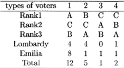
Table 1.1: Numerical Example Ranking Types per Region types of voters 1 2 3 4 Ranki A B C C Rank2 C C A B Rank3 B A B A Lombardy 4 4 0 1 Emilia 8 1 1 1 Total 12 5 1 2

the regional level (Lombardy and Emilia in the above example) and one at the national level. Under common knowledge, we solve this example by considering the only possible equilibrium if all voters are strategic. Each voter supporting either Party A or B will cast both votes for her favorite party. Types 3 and 4 instead may face a strategic dilemma. Their favorite party (C) cannot win so they may be tempted to cast a strategic vote. First, consider the Congress vote: since they know that the election is not close their dominant strategy is to cast the vote for C irrespective of their region of residence. In the case of Senate, the premium is given at the Regional level, so incentives are different for voters in different regions. The type 4 voter in Lombardy knows that she will be pivotal. Therefore her optimal strategy is to vote for B in the Senate election. Type 3 and 4 in Emilia instead know they will not be pivotal in the Senate election so they will vote C as they did in the congress ballot. Therefore the electoral outcome would be:

Table 1.2: Summary of Results for Numerical Example

Congress L Senate L Congress E Senate E

Party A 4 4 8 8

Party B 4 5 1 1

Party C 1 0 1 1

A+B 8 9 9 9

A (A + B) -1 0

Denote by

A

(A + B) = Votes Conress+Votes ongress) - (VotesSenate

+

VotesSenate). In this specific example we have A (A + B)Lombardy < 0 and A (A + B)Emilia = 0. More generally the prediction that we will be testing is: A (A + B)Lombrdy - A (A + B)Erilia <

0.Here,

we see that A (A + B)Lombardy

-A (-A+

B)Emilia =

-1-This negative sign reflects the fact that strategic voters are relatively more likely to switch to one of the top two parties in toss-up regions versus non toss-up regions.This simple prediction is generalized in the following Section and is at the core of our empirical specification.

1.3.2

A general set up

There are three parties (A,B,C) and two ballots (Senate and Congress). The majority premium is at the national level for Congress and at the Regional level for the Senate. C is never a likely winner neither in the national election nor in any region. We assume that there is common knowledge of the probability of being a pivotal voter at the national level 7r(a,/3) and at the regional level 7r0 (ay, 3).4These probabilities are derived from the distance in polls (a) and the size of the electorate in the region (/3). '

Each voter

t

is characterized by a vector ranking her preferences r over the three parties (e.g. A,C,B or B,C,A etc), and a region

j

to which she belongs. We summarize the characteristics of voter t with a tuple (r,

j,

&). Each voter casts two votes a, and as, one for the Chamber and one for the Senate. She has "warm

glow" utility J, from choosing her first ranked party and a different utility value for the various possible rankings of parties (to simplify we assume she only cares about the winner of that ballot). Therefore the utility when choosing a, for the congress elections and a, for the senate elections is:

U = 6J1 (a, = r (1)) +

(

v'l (Chamberwinner =

j)

z=A,B,C

4

Allowing these probabilities to depend on individuals' priors 7r(a, 3) would not change our results (as long as we assume common priors) but would introduce unnecessary complication.

5

Notice that it is obvious that lower alpha (more contested elections) means higher probability of being pivotal all else constant, while the same is not true for /. On one side lower population means that there are fewer seats awarded in the senate and so the overall probability of being pivotal in the senate goes down, but the fact that there are fewer voters also makes it more likely to be precisely the pivotal voter for constant a.

Us = 6j (a, = r (1)) + vIl (Senatewinner =

j)

z=A,B,C

Each agent has a different taste for his utilitarian pleasure from coherence (3L)6 We assume that it is distributed across regions with region-dependent distribution Fj over support [0, K]. We also assume that the ranking types (r) are identically distributed across regions and that v is the same for voters with the same ranking. That is

vi

= vVl E {A, B, C} as long as rk (M) = rz (m) Vm E {1, 2, 3} 7

We now show how the optimal strategies of such rational (strategic) voters would depend on the poll distance and the population of the region.

Remark 1. Voters whose favorite candidate is A or B, will cast a ballot for such candidate in both the Senate and the Congress irrespective of public information and their regional residence (j).

Proof.

See

Proof.

It remains to show how the C supporters vote.

Proposition 2. In every region j, and election ballot M - where N stands for national ballot and r for regional ballot from region r - there exists a cutoff 3"1

j such that all C supporters s. t. 6, <

3

' vote strategically am = r (2) and all C supporters such that 6, >

3

will vote sincerely am = C.

Proof.

See

Proof

Now remember that in our initial discussion we highlighted how smaller ctjs correspond to region

j

being more tossup. The effects of / instead depend on the underlying model used to describe 7r (a, 3).

Proposition 3. Under identical benefits distribution F across regions, if a region 1 is relatively more tossup than a region

j

(al < as) there will be relatively more misaligned voters, i.e.:

(F

(NJ)

-_ F

A

(Fj

(

3N,j) -Fj

r(ij'

<

0

.1

Proof.

See

Proof.

Remark 4. Note that this result depends on assuming identical distributions (F) across regions. An easy counterexample to the above theorem would be letting region

j

be more tossup than region 1 but assuming that the distribution of the benefits (J) is a Dirac measure concentrated on K while the distribution of Fj is uniform.

6

We do not actually need to have a behavioral assumption. Given that the system is proportional, it is enough that voters prefer to be a larger minority rather than a smaller minority.

T

From this little formal set up we can be pretty clear about what we should observe in the data:

" We should observe that the parties A,B receive more votes in the Senate relative to the Congress for the tossup regions relative to non tossup

* We should observe that A,B receive more votes when a is lower. " Unclear predictions for comparative statics on 3.

Our model predicts that all voters playing strategically will be supporters of party C. These are not the total strategic voters but just the misaligned voters. Strategic voters' estimates should be adjusted for the size of party C.

As highlighted before, our results might not hold if F differs across regions. It is reasonable to think that F is not constant across the country, but it is reasonable to believe that F is constant in municipalities within few km. In this case, geographic Regression Discontinuity would consistently estimate strategic voting.

1.4

Data and Empirical strategy

1.4.1

Data

We merge three municipalities data-sets on voting, social-economic background, and geographic coordinates. Furthermore, we use the most recent electoral polls , published by television broadcast Sky, to measure the level of strategic incentives at the regional level.

Voting data are provided by the Historical Office of the Italian Department of State ("Ministero degli Interni") and contain municipality level votes by party for both Senate and Congress. We aggregate the party votes into coalitions because this is the level at which the strategic incentives operate. We use electoral documents to classify parties into coalitions. Coalitions are the same for Senate and Congress across Italy and they are officially defined before the election. The parties within a coalition can vary across regions, but for any Region they are the same between Senate and Congress. For instance, the Center-Right coalition contains some regional parties that appeal to local pride. Since our identification looks at the shift of votes across coalitions between Congress and Senate at the Municipality level, this heterogeneity is not a concern. Italy is divided in 20 Regions and 8092 Municipalities. It is worth stressing that municipalities do not correspond to electoral districts, meaning that all the municipalities within a Region face exactly the same type of voting process. We drop from our analysis two regions: Valle d'Aosta and Trentino-Alto Adige. The reason for this choice is that the electoral rule in these regions is different from the standard one8 and

8

Valle d'Aosta (VA) and Trentino Alto Adige (TA) are two autonomous regions with a special statute. Therefore, the Constitution allows them higher legislative flexibility.

that local parties representing the interests of linguistic minorities play an important role in these regions. Dropping these two regions brings the number of municipalities used in the analysis to around 7700. We collect various demographic and economic data from the last issue of the "Atlante dei Comuni". This is published by ISTAT, the national Bureau of Statistics, and contains information at municipal level. ISTAT also provides us with cartographic information for all the Italian municipalities. We measure the distance of a municipality to the local regional borders using geo-coded information. The procedure we employ is the following. First, we use the coordinates of the border of each municipality to determine its centroid. Then, for each municipality, we define as the distance of the municipality to the border as the airline distance to the closest point of the border. We also compile manually a list of municipalities right at the border.

For poll data, we resume to official sources. The Italian government established a web-site9 where every media company is required to publish any public electoral poll. Using the web-site, we identified the poll that: (a) was closest in time to the election date; (b) had data on the intention to vote at regional level for the Senate ballot. While there are many pools in the period before the election, very few cover something different than the national result or a small subset of regions. The previous criteria led us to select the poll produced by the marketing company Tecne' for the TV broadcast Sky, one of the 3 biggest Italian TV group and subsidiary of the multinational group News Corporation'0. The results of the poll are provided in the appendix. Using this data, we construct an index to capture how tossup Region

j

was before the election:

Tossupj = -|CenterLeft - CenterRightjj

Where CenterLeft and CenterRight are the expected share of votes at the regional level for the two main coalitions in the Senate ballot. In other words, this measures how close the top-two coalitions are expected to be right before the election. The closest the index is to zero, the more toss-up a region is and therefore the more we should expect voters to engage in strategic voting, as predicted by the model. Notice that the index is always negative, therefore the higher the index, the more tossup the region.

1.4.2

Introduction to the Empirical Strategy

In an ideal randomized experiment on strategic voting, we would observe how the vote of the same individual changes under different beliefs about the probability of being pivotal. While not quite identical to an actual randomized experiment, the Italian Electoral system in 2013 had some features that made it very well suited to answer this question. First of all, Italy is a rare example of perfect bicameralism, where the two elected Chambers have exactly the same institutional role and they differ only on their size and the rules governing

9

http://www.sondaggipoliticoelettorali.it/

IOThe

poll is based on surveys run around February 11th, each poll is stratified at the regional level by the socioeconomic and geographical residence. Since two Regions had missing info, we fill the gap with the equivalent poll produced the week before by the same company, Tecne', for Sky.

active and passive electorate. A consequence of this perfect bicameralism is that any voter should have the same exact preference ranking across coalitions in the two Chambers. Comparing the share of votes going to each of the two Chambers we difference out the true underlying preference of the voters. More generally, the difference between the two reflects only factors that have an asymmetric effect across the two Chambers. Secondly, the "Pig Crap" law is characterized by a wide level of heterogeneity in strategic incentives across the two Chambers. While the seats in the Congress are assigned at national level, the seats in the Senate are assigned based on the electoral results at the regional level. We focus here on the incentives generated by the large majority premium assigned to the coalition receiving the largest share of vote in each region1 1. While the strategic incentive for the Congress is constant across the whole country, the incentive for Senate changes region by region, depending on the level of closeness of the two-contenders coalitions, which is measured by

our Tossup index. We exploit this geographical heterogeneity in our empirical strategy.

A simple model of strategic voting predicts that supporters of non contenders in toss-up Regions, will be relatively more likely to switch to one of the top two coalitions in the Senate ballot. This is the prediction of Proposition 3 of our model. The condition in Proposition 3 translates into the following linear equation, where we would expect the parameter 3 to be negative:

A-S

=

a

+

5

(TossUpj) + 3Xij

+ Eij

AC-S is the difference in the sum of votes for the two main coalitions between Congress and Senate, TossUp is an index that measures the level of closeness of the parties in the pre-electoral poll, higher values of the index imply more closeness, and Xij is a set of covariates at the municipality level. Under the assumption of no heterogeneity in preferences, the parameter

5

is a consistent estimator for the the share of misaligned voters for a given level of closeness in the electoral race. However, the assumption of no heterogeneity in preferences is very strong. If it fails, the least squares estimator for 6 is consistent if and only if the set of covariates Xij controls for all the observables and unobservables heterogeneity across municipalities. Here, we employ a geographical Regression Discontinuity setting to relax the identification assumption and provide evidence on strategic voting with high internal validity.

The intuition behind the Regression Discontinuity framework is the following. Consider comparing two adjacent cities, call them A and B, that are separated by a Regional border. Given that the population lives just a few minutes apart and given that there is full mobility of factors and people across Regions, we expect these two cities to be identical, both in observables and unobservable characteristics. However, the two cities crucially differ in the expectation regarding the results for the Senate race at regional level. Our test looks at how the difference in votes for the contenders' coalitions change as a function of the ex-ante perception on regional tossupness.

While we show that municipalities close to the border are similar in observables characteristics, Regional borders could be associated with discontinuity in other relevant dimensions not captured by our set of covariates. For instance, Municipalities across the border differ in the identity of the belonging Region. Italian Regions have an important role in public good provision and more broadly in the local economy. It follows that Regional institutions may be an important determinant of political orientation. However, this is not a concern for us: since both Chambers have exactly the same role in the political decision making and given that we focus on the difference in voting across the two, local specific fixed effects would not be a concern for our results'2

. The only threat to our identification comes from factors that affect the votes across the two Chambers and that are correlated with the Toss-up index presented above. Strategic behavior by parties is the main confounding factor we have in mind. In the last part of the paper, we argue that this concern is very unlikely to be first-order here, because of the electoral institutional features. Our estimates could be interpreted as a lower bound because the function that relates the number of strategic voters to the tossupness of the election could be non linear. By estimating the average effect over treatments of differing intensity the non linearity could lead to an underestimation of the percentage of strategic voters.

In the next Section, we discuss more in detail the empirical framework. After that, we focus on the most relevant case of difference in strategic incentives, the border between Lombardy and Emilia-Romagna. This example will help build intuition about the empirical framework as well as providing a plausible bound for our estimates. In the end, we present our main results and discuss robustness tests.

1.4.3

The Regression Discontinuity test at the National Level

In the setting of our analysis, there are a total of 27 Regional borders, for a total of 54 border-sides. Our empirical framework differs from the standard Regression Discontinuity framework because we have different boundaries where the treatment changes discontinuously but in potentially border specific ways. In the basic case, a forcing variable (distance from the border here) defines one relevant discontinuity and the test focuses on studying how the outcome of interest discontinuously changes across it. Here, we need to develop a test that is generalizable to the 27 borders. A notable example in the literature is Black (1999). She is interested in studying the effect of school quality on house prices, using school district boundaries in Massachusetts to identify the relevant causal effect. While her framework is particularly valuable because of its simplicity, it may lack in flexibility for a case where it is not possible to use observations exactly on the discontinuity. We therefore use a more general two-step framework, developed by Pinkovskiy (2013). As a robustness, we present our results also using a framework equivalent to Black (1999) and Dube et al. (2010), and we show that the results are unchanged and, if anything, statistically stronger. 13

12

TWo people with the same underlying preferences might have different political tastes at the national level in two regions or even just two municipalities that have different policies, but such preference would be reflected in the same (potentially different

between the two people) party vote at the Congress and Senate._{1 3}

A strategy similar to Dube et al. (2010) has been recently used in Naidu (2012), where fixed effects per pairs of counties are added to isolate the effect of state level law changes.

The intuition behind the Pinkovskiy's procedure is simple. Different borders may differ in their size, density of municipalities and dependence of the outcome on the forcing variable. Therefore pooling together the whole set of municipalities at the border may not be the cleanest procedure. One way to look into this is to aggregate at border-side level the information. This is what we do here. In a first stage, we estimate the conditional expectation at the border of our outcome variable AC-S separately for each border-sides set of municipalities. In the second stage, we use these estimates as outcomes in a cross-sectional regression on the level of closeness in the regional race, Tossup. In practice, we start by estimating the following equation for each border-side separately:

AC-S -gs

+

p(dij)

+

fij

This is estimated over the set of all municipalities that are within a bandwidth of B km from the relevant border, assuming p as linear. Notice that

Eg-

is simply the constant of the least-squares estimator and it estimates the conditional expectation of the outcome variable at the border (d = 0). Since we estimate a different function per each border-side, we allow total flexibility on the conditional expectation across border-sides. Then we use these estimates in a second stage as outcome. In particular we estimate:

AC-s =

a

+6Tossupj +

0,j

+

e

where

1k

3 are the conditional expectation of the standard covariates at the border14. The observations are

weighted by the number of voters at the border-side. Given the definition of the variables, the theory predicts that J should be negative in presence of strategic voting. The standard errors in this model are clustered at the border level. In the result section, we discuss some relevant specification robustness, such as allowing for border specific fixed effects.

This framework as any other Regression Discontinuity requires two important assumptions. First, we need that every relevant factor different from the main outcome is a smooth function of distance across the discontinuity. In the result section, we show this is actually the case for a set of important covariates. This is not surprising, since the sets of municipalities that are compared are usually very close and regional border do not determine any relevant change in labor markets institutions, credit or infrastructures.

Second, we need to make sure that our results are not simply driven by sorting of citizens across the border. Lee and Lemieux (2009) argues that sorting is probably the first order concern around geographical Regression Discontinuity. People can choose where to live based on their own preferences and characteristics. If the endogeneity of the choice is related to the mechanism we are testing, then our estimates could be biased. Luckily, we can strongly reject this criticism. In this context, it is highly implausible that the location choice

can be related to voting behavior as described in our model. In Italy, voters need to vote in the Municipality where they are resident. Changing the Municipality of residence is costly and time consuming15 and therefore it is highly unlikely that anyone would undertake this process for the small and uncertain gains from strategic voting.

It is important to make the following point about inferences. Pinkovskiy (2013) argues that the standard type of asymptotic, where data are independently generated with the number of observations going to infinite, may not be particularly well suited for the case of geographical Regression Discontinuity. He proposes a new estimator for the variance under infill asymptotic. In the standard asymptotic, the domain from where observations are drawn is thought to go to infinite: with infill asymptotic instead we have that resolution of our data increases to infinity. In our setting, this would be equivalent to have data on votes for infinitely smaller municipalities. He shows that, when infill data are used and errors are correlated, the standard variance estimator is too conservative. While we believe the analysis presented by Pinkovskiy (2013) is of great interest and deserves more exploration in the future, in our work we decided to use the standard White estimator for the variance. There are two, related reasons why we make this choice. First, the typical standard errors are overly conservative and therefore they would prudently bias us against finding any statistical significance. Secondly, the actual properties of the estimator of the variance proposed by Pinkovskiy (2013) are not well known in finite sample.16

1.4.4

A case study example: Lombardy vs. Emilia-Romagna

We start the presentation of the results, by looking at the border between Lombardy and Emilia-Romagna. This case study is important for multiple reasons.

First of all, it helps exemplifying the intuition behind the Regression Discontinuity approach. Secondly, this border represents the cleanest example of discontinuity in strategic incentives, because it compares one almost perfectly toss-up Region (Lombardy) with one where the electoral result was completely uncontested (Emilia-Romagna). According to the most recent polls before the election, in Lombardy Center-Left and Center-Right were expected to be tied. Elections were expected to be decided by thousands of votes and the strategic importance of this area was particularly stressed by media and politicians. Instead, Emilia-Romagna was, together with Tuscany, the least contested Region in Italy. The Center-Left was expected to lead the race by at least 20 percentage points. Historically, the communist party first and the center-left coalition afterwards had always won the election in this area post World War II. Lombardy was not only more contested, but, because larger than Emilia-Romagna in population, its victory was more determinant

15

Voters need to apply to the new Municipality much in advance than the Election, providing a proof of residence in the new Municipality. Local police then need to validate the information provided by inspecting the new residence. The whole process may take weeks, if not months, and it requires filing multiple forms and paying some fees

161n

applying its theoretical framework to his empirical problem, Pinkovskiy (2013) develops a routine where he uses either the White or its own variance estimator depending which one is smaller. The idea is that the variance he develops is always smaller than the standard White estimator in asymptotic, but this may not be in finite sample. That's why choosing White standard errors is more conservative in our setting.

for the final outcome. Ali in all, the

expected

valie of voting strategicalty was characterized by a large julijp across the )order.

In

t Ini Ihis

cas

is particularLy interesting because it. provides an upper bound for

the size of strategic voling.

Since we are coiparing the most contested with the least contested Region,

the

probability of beiig pivotal is characterized by a. sharp discontinuity at this border. However on other dimensions the two Regions appear to be quite similar at the border. Lonbardy and Emilia4Roimagnia are the ttwo richest Regions of

Italy,

among the richest in Eturope. While quite d1ilferetut iii many instances, alona the border their dif

erns

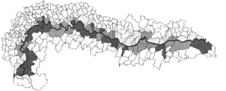
shrink. C onsider for instance, the subset of Municipalities Which are Cxactiy on thw border between Lonibardy and Eiilila-Roiagna. This set of 83 M\lunicipalitis is the

closst

you (,in get to an ideal Regression Discontinuity

(igoure -4). By constructlion,

every

Municipality at one side of the border is

contiguous

with at

least

another Municipality in the (counter-factual) Region. Consider the heat map presented in

figure

-5. where the running

variabl is income per person. Income dces not appoar to be characterized by any discontinuity across the border. In fact, if anything, the spatial distributlion of inconie seems to be characterized by clusters along

the boner, with Municipalities with similar

income

grouping together across the border. This pattern is not unique of tie Municipalities along the border, but the results do not change when considering wider bandwidth around the border

line

(look figure figure -6 for same with a

10km

bandwidth). Furthermore, results are qualitative similar when considering other outcomes.

Figure 1-1: Distribution of Income by Municipality, Lombardy vs. Emilia-Roniagna.

Notes: this map

contains

all the Municipalities in Lombardy or Emilia-Romagna, that are within

0kn

from the other Region border. Colored are the MNiicipalities that are on the border. A darker color signal higher level of income per capita in that

figure

1-2:

Distribution of the outcome by Municipality, Lombardy vs. Euilia-Roiagna

Notes: this map contains all the \iunicipalities in Lombardy or Liilia-Romigni, that are within 1tkm from the other Region 1boirder. Colored are the MMiiiti at are on the o1rder. A Arker rotor siginil higher level of' the ontcoine variable, which is the difFerence in the share

or

votes going to one of the top-two CoalItions utween Cng ress and Snate at MNunicipality level.

Data on incnie are provided by Italian Department of State. The black line is the border btiMen tl two Regoms.

However, thc Aor= is hiltrent win we look at 0ur outoume variable

A

-is input in the heat map

figure -6).

Lere

inst thiii[le discofntiuit is

qtuitt

x

evident.

The Municipalities in the north side

of

the border

appear to have oii average a larger share of voters voting for the fwo contenders

coalitionis

ill Senate than in Congress. The result is confirmed when looking at different bandI) widths.

The story at this point is

clear:

Mimicipalities at the two borir diilUr by the level of incentives for heing

strategic, but they tend to be very hollmogeiious along other dimiiiensions. While the case of Lonibardy versus

lmilia-Roiagna cannot Ibe generalized furtlier, the bottomt

line

is confirmed by further tests ill

the national

sample. As we will show, in fact, the level of pivotality of regions does not appear to be correlattd with values of

covariates

at the discontiimlty.

The results presnt-ued graphica'lly

cali

also be confirned in a formal specifiation. Ve consider four samptes. We

s tart

considering what we think is the closest to the ideal RD setting, which is the case where we analyze only the 1ehavior of MunIuicipaitis right Ht the border. We tleii consider Wle set of Municipalities whose

cenlroids

ar a

t

1035, and 20 kmi froni

the

border. Results will he both quailitative and quantitative similar

across

the

different samples. W"'o run a simple linear local regression, where we study how being in the iore toss-up Region (ILoibardy) afftcts it lthavior of voters in close-b-xy Municipalities

The results alln be found in talilc

5.

Crossiig the border of Etilia-Roimagna and

Lombardy

implies a drop in

the

outcorn nariable of about

1.5%.

Iter we discuss how to recover the

extent

of stra-tegic voting from these estiinates, under quite iiild assumptions.

iln

this case, it is

only

wxortlhv to point out that these estinates imply a nmaxininin extent

of

strategic voting around

5%

once we correct for misaligned voters. While still

substantial and potentialty relevant, this is vnery far from previous work. In Cohuin (1) we present the

T[he euprtion of interest is tih following:

-= +5Lombardy + p(d ik) +<

wshimere d

u-

is tte Wistance Ni Miniiipalty i to the irdt-r bttwin j and k, and pis assmned to he linear and different at the

simple coefficient with the border regression, where no correction for distance and covariates is applied. In Column (2) to (4), we subsequently add controls and distance functions18. Results are stable. Notice that in Regression Discontinuity, adding controls is not required for identification. We add them here mostly for robustness and to gauge the precision of our estimates. In the end, between Columns (5) to (7), we present the results for the different distances, and in particular for all the Municipalities within 10,15, and 20 km from the border. Again, the results are not statistically different from each other and in line with what expected. In the end, in the appendix we present a formal test for the conjecture of balancing of the covariates (see table 6). For all the sub-set of data, we do not find any statistical differences across the border in relevant outcome variables.

1.4.5

Results and Robustness

We now generalize our previous test to the whole country, by employing the two-step procedure develop by Pinkovskiy (2013) and presented above. We start by showing that our Toss - up3 index does not

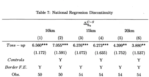
systematically predict differences in other covariates at the border - the extension of the test we already performed for Emilia Romagna and Lombardy. Results in this direction can be found in the appendix (see table 8). In particular, we test whether the conditional mean at the border of the covariates appears to be correlated with the toss-up score. Of all variables, only the size of the population appears to be significantly correlated; only when considering a bandwidth of 20km and only at the 10% level. So the test confirms the balancing assumption for the national sample.

We estimate our two-step estimator in three sub-samples, looking at bandwidth of 10,15, and 20 km from the border. We show these results in table 7, where we report every specification both with and without controls. As expected, the introduction of the controls does not substantially change the value of the estimated & but it reduces standard errors. The specification confirms the results provided for Lombardy, where the more toss-up sides of the borders tend to have a larger share of voters acting strategic than their counterparts. In the next Section, we discuss more in detail the interpretation of the magnitude of these coefficients. One concern with this procedure is that, the density of Municipalities close to the border may be particularly low in some specific borders. While this is not a big concern when considering a 20km mile bandwidth, it can be a problem with the 10km border. For instance, with the 10km bandwidth we were forced to drop two borders (Emilia-Romagna vs. Piemonte and Marche vs. Lazio) in the first-stage. We try to address this concern in two ways. We start by expanding the bandwidth in our first stage up to 30km from the border, in order to test the sensitivity of the model to number of observation in the first-stage. Our results are always in line with our main specification. Then, we implement a non-parametric bootstrap, in order to test '8Notice that the border regression is the closest you can get to the ideal RD. Here controlling for distance makes little sense, since the function of distance do not really discriminate between Municipalities that are closest or further from the border-since they all are on the border but rather between Municipalities whose centroid is closest or further from the border. Since we do not know the population distribution within the Municipality territory, this type of discrimination would be arbitrary.

whether our conclusions may be somehow driven by small sample bias. For every iteration i, we randomly draw with replacement N observations from the sample of N Municipalities within B km from the border. This is done completely independently for each of the 54 border-sides. Then, we use this sample to estimate the 0) following the usual procedure. Using the empirical distribution of {0)

000,

we estimate confidence interval for the parameter. Again, all results are confirmed. All these tests can be found, as well as other robustness, in the appendix of the paper (see table 11).

Our estimates 6 exploits the cross-sectional variation in the level of the toss-up index and Ags, while

%ij

creating a balance sample of homogenous areas. Alternatively, we may instead consider a different estimator, where we exploit only within border variation through the introduction of a border-specific fixed effect19. This estimator compares how, within the same border, differences in the tossup level affect the share of misaligned voters. If our primary specification is correctly specified, then we would expect this test to substantially confirm our previous results. This is what we find in the data. In the new fixed effects specification, the magnitude of 6 is around 20% larger, and still highly significant. While larger, a formal test reveals that the two parameters are not statistically different between each other.

As a concluding robustness to our results, we present a simple one-step equivalent of our two step estimator. In particular, we pool together all the Municipalities that are within a distance B to the border for the whole 27 borders and we test whether being in a more toss-up Region affects the voters' strategic behavior. This is very similar to the methodology used by Black (1999) and Dube et al. (2010)20. While our two-step estimator is more flexible in controlling for the differential effect of distance across different borders, their estimator is more parsimonious. If the relationship between distance and outcomes is not particularly heterogeneous across border-sides, we expect this specification to produce estimates close to the one in the two-step estimator. The results presented in table table 11 confirm our previous findings. If anything, these estimates seem to be even smaller than the one with the two-step estimator.

1.5

Discussion

In this section we show how we can recover from our previous estimates the extent of strategic voters. Furthermore, we discuss the role of strategic parties in our setting and in the interpretation of the results. So far we estimated the effect of the level of electoral contestability on the size of misaligned voters2 1. Because citizens from the main parties face no strategic incentives, the total misaligned voters represents the amount of strategic voters within secondary coalitions. To get back an estimate for the total strategic

19The specification is

E

S =ab() 6Tossup₃ +

#X

3 +

ej,

where is a border fixed effect, which is the same level of

clustering of our standard errors.

20

We estimate ACS = c + 6Toss - up₃ + p(dij) +

e

3 over the whole set of Municipalities within a bandwidth B to the

border

2 1